Localized and Short-Term Effects of Lockdowns on Urban Rental Markets: Evidence From Shanghai
ABSTRACT
This paper investigates the localized and short-term effects of COVID-19-induced lockdowns on Shanghai's rental market in the second half of 2022. Using Difference-in-Differences methodologies, we find that rental prices declined by 1.5% following the lockdowns on average, with areas characterized by a high density of companies falling by 2.0% and no significant change in suburban areas. Event-study analysis further reveals that this decline peaked at 3.0% 2 months post-lockdown. This decline was temporary with rental prices returning to pre-lockdown levels within 12 months. Robustness checks and comparisons with housing sale prices confirm the absence of significant spillover effects or structural shifts. These findings underscore the localized and temporary nature of lockdown-induced disruptions in the rental market and may be valuable to housing policymakers considering responses to short-term crises.
1 Introduction
The COVID-19 pandemic has profoundly impacted urban economies and housing markets worldwide, sparking considerable interest in examining how pandemic-related policies, particularly lockdowns, have influenced housing dynamics. Specifically, many studies have examined the “donut effect”, in which lockdowns and remote work prompted households to move from densely populated urban centers to suburban or rural areas (Duranton and Handbury 2023; Pawson et al. 2022). This phenomenon has driven significant and enduring shifts in housing preferences: suburban markets have often experienced sustained growth, while urban rental markets have struggled to recover (Kuk et al. 2021; Ramani and Bloom 2021). In this paper, we investigate the impact of the COVID-19-induced lockdowns on Shanghai's rental market in the second half of 2022 and find that the effects of the lockdowns were localized and short-lived, thereby challenging the prevailing narrative of long-term structural changes observed in other contexts.
Our study finds that the lockdowns significantly impacted areas with a high density of companies, with rents falling by 2.0% on average in the 4 months following the lockdowns—an effect that persisted for approximately 11 months. This aligns with research emphasizing the vulnerability of areas with concentrated economic activity to external shocks, where reduced business operations and employment opportunities directly affect housing demand (Ramani and Bloom 2021; Ahrend et al. 2023; Beze and Thiel 2025). We find that suburban rents remained stable, which is consistent with the literature on urban resilience, suggesting that areas less dependent on commercial density and employment fluctuations are less impacted by shocks (T. Li et al. 2023; Guglielminetti et al. 2023). Furthermore, the temporary nature of these effects—evidenced by the return of urban rental markets to pre-pandemic levels within 12 months—is consistent with research highlighting the ability of rental markets to rebound after short-term economic disruptions (Gupta et al. 2022; Sequera et al. 2022; Batalha et al. 2022). These findings suggest that the observed rental price dynamics are driven by a localized decrease of economic activity rather than a structural shift in housing preferences.
To estimate the causal effects of lockdowns, we employ a robust empirical strategy, utilizing data at the geographic point-month level, which includes detailed rental data from Beike.com, geospatial business density data from AutoNavi Map, and official lockdown records detailing medium- and high-risk areas (risk area definitions discussed later). We apply a Difference-in-Differences (DID) framework alongside event-study analyses to assess how rental prices responded to lockdowns. Additionally, by categorizing areas into high- and low-density companies groups based on the spatial distribution of companies and integrating lockdown records, we incorporate density heterogeneity in the DID model to estimate the impact of lockdowns on rental prices for different density groups. Our approach addresses potential biases, such as geographic imbalances and spillover effects, by employing propensity score matching (PSM), placebo analyses, and incorporating secondary housing price data. These rigorous methods enable us to isolate the temporary and localized effects of lockdowns on rental prices and offer a nuanced understanding of how urban and suburban housing markets respond to external shocks.
Our results demonstrate that lockdowns had a significant impact on rental markets in Shanghai, with distinct differences between high-density business areas and suburban regions. Under the baseline DID framework, we find that rental prices decreased by approximately 1.5% on average during the 4 months following the lockdowns. The accompanying event study further substantiates these findings, showing that the rental price decline in high-density areas peaked at approximately 3.0% 2 months after the lockdowns. Incorporating heterogeneous analysis, we further find that rental prices in high-density business areas decreased by approximately 2.0% on average, while suburban rental prices exhibited no statistically significant change. This decline was temporary with rental prices returning to pre-lockdown levels within 12 months, as suggested by the extended period analysis until December 2023. These results suggest that the rental price decline was more pronounced in urban centers with higher business activity, where lockdowns led to a sharper reduction in housing demand due to economic disruptions and employment losses. In contrast, suburban rental markets remained stable, underscoring their resilience to such shocks.
This study contributes to three strands of literature. First, it contributes to the expanding literature on the impact of the COVID-19 pandemic on urban housing markets (e.g., Ramani and Bloom 2021; Ahrend et al. 2023; Beze and Thiel 2025). While much of this literature has focused on long-term structural changes, such as suburbanization and shifts in housing preferences, our study demonstrates that these effects may not be universal. By showing that rental price declines in Shanghai, induced by the lockdowns, were both localized and short-lived, we emphasize the contextual nature of pandemic-induced housing market dynamics, which are shaped by local economic and governance structures.
Second, this study extends research on the heterogeneity of housing market responses to external shocks, such as economic recessions and natural disasters (e.g., Gupta et al. 2022; Sequera et al. 2022; Batalha et al. 2022). Our findings emphasize the importance of business density heterogeneity, demonstrating that high-density business areas are more vulnerable to short-term economic disruptions, while suburban areas remain relatively insulated. These findings strengthen the evidence base for understanding the mechanisms driving housing market resilience in different urban contexts.
Third, this study contributes to the literature on urban development and resilience (e.g., Glaeser 2022; Batty 2016). Urban resilience refers to a city's capacity to absorb and recover from shocks, such as economic disruptions, natural disasters, or pandemics. Our findings demonstrate that rental markets, while initially affected by economic slowdowns, exhibit strong recovery potential. This insight into how urban areas recover from crises could be valuable to housing policymakers considering responses to short-term crises.
The structure of this paper is organized as follows: Section 2 introduces the background of COVID-19 lockdowns in Shanghai and provides an overview of rental price trends across high- and low-density areas during the study period; Section 3 describes the data and provides summary statistics; Section 4 outlines the empirical strategy, including the baseline DID approach, a DID model with density heterogeneity, and the event-study for the baseline DID; Section 5 presents the main results, highlighting the localized effects of lockdowns on rental prices, as well as robustness checks, spillover analyses, and comparisons with housing prices; Section 6 further explores the long-term effects and discusses the correlation between migrant population outflow and rental decline; Section 7 concludes.
2 Background
2.1 The Pandemic in Shanghai 2022
In 2022, Shanghai faced a severe COVID-19 outbreak, which led to a citywide lockdown, followed by targeted partial lockdowns in specific areas. These restrictions lasted for 6 months, until nationwide pandemic control measures were lifted on December 20. As confirmed cases surged starting February 28, the city started citywide lockdown on March 28. By May, new COVID-19 cases had decreased by nearly 80%. To balance pandemic control with economic recovery, Shanghai began easing the citywide lockdown on June 1, while maintaining localized three-tier control measures which classified the city into low-, medium-, and high-risk areas based on active transmission levels.
This study focuses on the period from June to December 2022, during which Shanghai implemented partial lockdowns in response to localized COVID-19 outbreaks. Lockdown orders were issued dynamically, based on the emergence of new cases in specific locations. When a positive test result was confirmed, the locations visited by the individual were assessed to evaluate potential transmission risks. Areas with additional positive cases detected during screening were classified as “medium-risk” or “high-risk” zones and placed under lockdown. These “risk areas” typically referred to specific communities,1 workplaces, or buildings. The Health Commission and the Centers for Disease Control and Prevention coordinated public notifications regarding risk areas through multiple channels, including press conferences, official websites, and daily updates on WeChat. This communication strategy ensured the timely and accurate dissemination of information about the pandemic's progression and related lockdown measures.
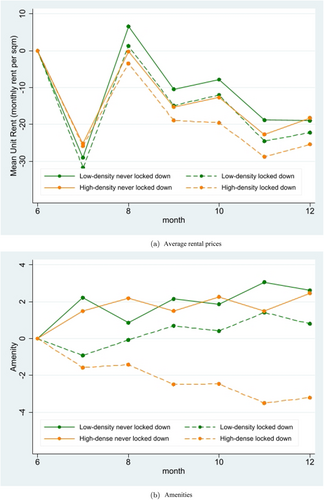
2.2 Deviation of Amenities in Central Areas With Lockdowns
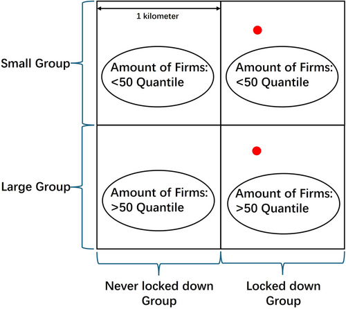
To investigate the impact of the pandemic on central and suburban real estate markets, we divided Shanghai into 1221 1 km 1 km grids and classified them into four categories based on business activity levels (high-density vs. low-density) and lockdown status (never locked down vs. locked down), as illustrated in Figure 1. Specifically, the number of local businesses in each grid was used as a proxy for commercialization, categorizing areas into high- and low-density groups. Using lockdowns data released by the Shanghai government, we further identified grids with no lockdown (never locked down group) and those with at least one lockdown (locked down group) between June and December 2022.
3 Overview of Data
Our primary research incorporates three distinct data sources: housing rent data, digital map point-of-interest (POI) data, and lockdowns order data, all of which are at the geographic point-month level.
Housing rent data: To analyze variations in rental prices, we collected monthly listings from Beike.com, one of Shanghai's largest online real estate platforms. According to Beike's prospectus, the platform holds a 9.7% share of the residential market, ensuring the data's representativeness. Our data set consists of 68,365 rental listings recorded between June and December 2022, with around 10,000 new listings added each month. For each listing, we obtained detailed information on rental prices, floor area, district, neighborhood, and geographic coordinates (longitude and latitude).
Digital map POI data: To understand the spatial distribution of commercial activity in Shanghai, we collected enterprise POI data from AutoNavi Map, one of China's most widely used electronic mapping platforms, in June 2022. The data set includes 69,699 points categorized as enterprises within AutoNavi Map's regional POI classification, with the first three digits of the six-digit category code being 170. Each record contains detailed information, including the unique AutoNavi Map ID, enterprise name, business type, registered address, phone number, and geographic coordinates (latitude and longitude). As shown in Table A1, these data represent enterprises across various sectors.
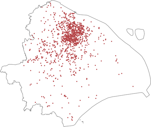
Lockdown order data: We obtained official information on the lockdowns of medium- and high-risk areas, including the lockdown start date and detailed addresses, from the National Health Commission's official website. Distinguishing between high-, medium-, and low-risk areas is one of the strategies China employs to prevent and control the COVID-19 pandemic. Specifically, high-risk areas typically refer to locations with a sharp increase in cases, while medium-risk areas are more broadly defined, usually characterized by a low number of infections but still presenting some risk of transmission (Wu and McGoogan 2020). During our study period, “risk areas” typically referred to communities, workplaces, or buildings. These medium- and high-risk areas will remain under lockdown until they are downgraded to low-risk status. In parallel, businesses such as restaurants, companies, and markets located in these areas would be closed for at least 7 days. Finally, we geocoded the medium- and high-risk areas, as shown in Figure 3.
3.1 Summary Statistics
The summary statistics of the listings (June–December) and 1 km 1 km grids, grouped by business density and lockdown status, are presented in Table 1. In Panel A of the table, “Unit Rent” is calculated by dividing the rental price by the house area. “Distance to City Center” and “Distance to Subway Station” are derived based on the distance from each sample house's community to Shanghai's center (defined as People's Square in this paper) and the nearest subway station, respectively, using the RANN package in R. In Part Two, the “Number of Risk Areas” represents the total count of risk areas within the grids of each group from June to December. The “Average Frequency of Risk Areas” is calculated by dividing the number of observed risk areas during this period by the remaining months after the first lockdown (i.e., December minus the month of the first lockdown), reflecting the average monthly frequency of risk areas from their initial occurrence to the study period's end. The “Number of Companies” refers to the total count of AutoNavi Map POIs classified as companies within each group's grids.
| Low-density group | High-density group | Total | |||
|---|---|---|---|---|---|
| Variables | Never locked down | Locked down | Never locked down | Locked down | |
| Panel A: Rental price | |||||
| Number of rental listings | 16,894 | 16,492 | 9632 | 25,347 | 68,365 |
| Unit rent (monthly, yuan/m2) | 105.86 (57.27) | 115.77 (56.69) | 134.89 (62.31) | 153.01 (60.82) | 129.82 (62.42) |
| House area (m2) | 64.94 (40.56) | 60.63 (38.24) | 63.35 (42.21) | 62.21 (41.07) | 62.66 (40.47) |
| Distance to city center (by community, km) | 18.54 (9.61) | 13.52 (6.77) | 11.96 (7.39) | 6.90 (5.47) | 12.08 (8.57) |
| Distance to subway station (by community, km) | 1.35 (2.05) | 0.98 (0.76) | 0.82 (0.93) | 0.55 (0.33) | 0.89 (1.20) |
| Panel B: Grid feature | |||||
| Number of grids | 557 | 224 | 236 | 204 | 1221 |
| Number of risk areas | — | 1.96 (1.60) | — | 2.79 (2.41) | 0.87 (1.66) |
| Average frequency of risk areas (following the initial occurrence and in subsequent months, month) | — | 2.83 (1.93) | — | 2.63 (0.65) | 2.73 (0.60) |
| Number of companies | 9.63 (6.44) | 11.62 (6.77) | 47.69 (24.29) | 58.52 (29.91) | 25.52 (26.79) |
- Note: The table summarizes the rental listings and 1 km 1 km grid features grouped by business density (high-density vs. low-density) and lockdown status (never locked down vs. locked down).
The summary statistics reveal notable differences across the groups. While the four groups are balanced in terms of house area, significant disparities exist in other characteristics. High-density groups are located closer to the city center and subway stations, have higher unit rents, and exhibit greater levels of commercialization compared with low-density groups. Additionally, locked down groups are situated in more central areas than their never locked down counterparts. This imbalance reflects a characteristic of Shanghai's pandemic dynamics: as shown in Figure 3, the central area recorded higher case numbers than peripheral regions due to its higher population density and more intense commercial activity. However, it is important to emphasize that, although the city center is more prone to pandemic spread than the suburbs, the manifestation of such spread, both in terms of time and space, remains random and unpredictable within the city center or suburban itself. To address concerns about potential imbalances that could threaten identification validity, we implemented two mitigation strategies: (1) incorporating community-level fixed effect to control the noise in rental prices, and (2) applying PSM based on the distance to the city center and the number of observed pandemic cases, in addition to the baseline estimation.
4 Empirical Approach
Our identification strategy compares listings' rental prices in areas that have experienced lockdowns with those that have not. Listings located in grids affected by lockdowns are assigned “treated” status, while those in unaffected grids are designated as “control.” We first use a baseline DID specification to estimate the impact of lockdowns on rental prices. To further examine the varying effects of lockdowns across areas with different company densities, we introduce heterogeneity into our DID model, allowing us to quantify the differential impacts on low- and high-density areas.
4.1 Treatment and Control
We define treatment status at the level of the grid-month: if a grid-month is treated then all the rental listings in that grid, in that month, are treated. A grid becomes treated once there is a single lockdown in a given month and then remains treated for the rest of our study period. Control grids are those that have not yet had a lockdown. Thus control grid-months consist of grids that were never locked down from June to December, as well as the pre-lockdown months from grids that were eventually locked down.
Given the relatively short duration of the initial lockdown, one might be concerned that early treated areas recover within the duration of our study, and thus their treatment status should revert to untreated after some period. However, the average frequency of lockdown in a region, following the initial lockdown and in subsequent months, is approximately 2.7 months, with 52% of regions experiencing multiple lockdowns. This aligns with the high transmissibility of the pandemic. Moreover, we contend that lockdowns suppress local economic activity, reduce mobility and opportunities, and increase uncertainty, all of which constitute negative shocks that necessitate time to recover. Assigning “treated” status solely for the initial lockdown month would overlook the cumulative and persistent effects of subsequent lockdowns. To further address concerns regarding this categorization, we refine the baseline regression window to encompass a 7-month period, including 3 months before and 3 months after the first lockdown. By restricting the analysis to this narrower time window, we aim to mitigate potential biases arising from long-term or unrelated shocks and focus more precisely on the immediate effects of lockdowns on rental prices.
4.2 Identification Strategy
5 Result
5.1 Baseline Lockdown Effects on Rental Price
We begin by investigating the effect of the lockdown on rental prices through the estimation of Equations (2) and (3). The final regression sample includes 52,912 observations. A total of 4487 samples were removed due to always treatment, 396 singleton observations were dropped, and 10,570 samples outside the regression window (i.e., outside the 3 months following or preceding the lockdown) were excluded. As shown in Panel A, Column (1) of Table 2, which reports the baseline results from Equation (2), the average rental price in the high-density group fell by 2.0 yuan/m2 (equivalent to a 1.5% decrease) in the 4 months following the lockdown. The heterogeneous effects for the low- and high-density groups are presented in Column (1), Panel B, based on estimates from Equation (3). These results indicate that the average rental price in the high-density group declined by 2.9 yuan/m2 (equivalent to a 2.0% decrease), while the low-density group increased by 0.3 yuan/m2, which is small and statistically insignificant. This suggests that lockdowns in central areas significantly reduced residents' willingness to live there, while having minimal impact on suburban areas. A plausible explanation for this disparity is that central areas, which typically offer more employment opportunities, were more heavily affected by the disruption of business activity and jobs after the lockdowns, leading to greater declines in rental demand compared with suburban areas.
| (1) | (2) | (3) | (4) | (5) | |
|---|---|---|---|---|---|
| Baseline | PSM | Spillover | Housing | Placebo | |
| Variable | Unit rent | Unit rent | Unit rent | ln(Unit price) | 2023 Unit rent |
| Panel A: Baseline | |||||
| All samples | −1.992*** | −1.665** | −0.142 | −0.00759 | 0.996 |
| (0.712) | (0.803) | (0.731) | (0.005) | (0.627) | |
| Observations | 52,912 | 45,076 | 26,526 | 15,097 | 46,769 |
| Month fixed effect | Month | Month | Month | Month | Month |
| Location fixed effect level | Community | Community | Community | Community | Community |
| Panel B: Heterogeneity | |||||
| Low-density group | 0.338 | 0.045 | 0.0463 | −0.00894 | 1.343 |
| (1.063) | (1.182) | (1.307) | (0.008) | (0.896) | |
| High-density group | −2.855*** | −2.688** | −0.282 | −0.00766 | 0.657 |
| (1.079) | (1.070) | (0.858) | (0.016) | (1.160) | |
| Observations | 52,912 | 45,076 | 26,526 | 15,097 | 46,769 |
| Month fixed effect | Month ∗ Group | Month ∗ Group | Month ∗ Group | Month ∗ Group | Month ∗ Group |
| Location fixed effect level | Community | Community | Community | Community | Community |
- Note: The table presents DID coefficients and their standard errors from models assessing the impact of lockdowns on dependent variables, with community fixed effects and month fixed effects in Panel A, as well as DID coefficients and their standard errors from models estimating the heterogeneous impact of lockdowns on dependent variables of both low- and high-density groups, with community fixed effects and month-by-group fixed effects in Panel B. Columns (1)–(5) correspond to the baseline, propensity score matching, spillover analysis, housing price examination, and placebo test, respectively. Standard errors are clustered at the grid level (or at the community level in Column 3), consistent with the treatment.
- Abbreviations: DID, Difference-in-Differences; PSM, propensity score matching.
- ***
- **
- * .
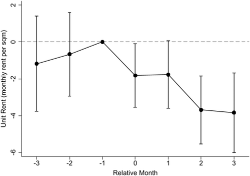
To investigate the role of pretrends and any dynamic effects of the lockdowns, we next present results from the corresponding event-study specification by estimating Equation (4). As shown in Figure 4, which includes 95% confidence intervals, there is no trend in the rental prices before the lockdown. And after the lockdown, there was a clear downward trend in rental prices. Moreover, the effect grew over time, rising to 3%, or approximately 4 yuan/m2, after 2 months of lockdown. These findings reaffirm the significantly impacts of the lockdown on rental price.
5.2 Lockdown Effects Under PSM
To further mitigate concerns that the never locked down group may be closer to the city center, potentially confounding the identification process, we employ PSM to select appropriate samples. Specifically, we regress both the distance from each grid to the city center and the number of pandemic cases within the grid to ensure the propensity scores of the control (never locked down) and treatment (locked down) groups are comparable. The details of this regression analysis are provided in Table A2. On the basis of the predicted propensity scores, we exclude approximately 15% of the samples, removing 3160 observations from the never locked down group and 6896 observations from the locked down group.
Using the refined sample obtained through PSM, we re-estimate Equations (2) and (3), with the results reported in Column (2) of Table 2. As shown in Panel A, the average rental price fell by 1.7 yuan/m2, slightly less than the baseline result, but still statistically significant at the 5% level. In Panel B, the effect of lockdown on the high-density group is estimated at 2.7 yuan/m2, which is also statistically significant at the 5% level. Meanwhile, the low-density group shows a small, statistically insignificant increase, consistent with the baseline results. These findings, derived from the PSM sample, are consistent with the baseline results in terms of both magnitude and statistical significance, further validating the robustness of our identification strategy.
5.3 Assessing Possible Spillover Effects
A critical question arises regarding whether our findings show spillover effects. Specifically, if a lockdown in central areas reduces an individual's willingness to rent locally, then they may choose to rent in nearby areas without a lockdown. To assess potential spillover effects, we calculated the distance from the never locked down group listings to the nearest locked down grid. We ranked the control group samples by their proximity to the nearest treatment group and categorized those below the 50th quantile as “near the treatment group” and those above it as “far from the treatment group.” This approach allows us to examine spillover effects within different proximity ranges. If spillover effects exist, we would expect to observe a significant increase in rental prices for rental listings near the treatment group. For listings in near the treatment group, we assume their treatment timing aligns with the timing of the nearest locked down grid. The summary statistics for these reclassified groups are provided in Table A3.
Using this adjusted data, we re-estimate Equations (2) and (3) to examine spillover effects. The results present in Column (3), Panel A of Table 2, show no significant increase in rental prices for listings near the treatment group areas compared with those located farther away. Additionally, we observe no increase in rental prices in Panel B, indicating that there was no change in either the high-density or low-density group. This finding suggests that spillover effects, whether driven by geographic proximity or differences in firm density, are negligible. Therefore, the impact of lockdowns on rental prices appears to be localized to the directly affected areas, without influencing nearby regions.
5.4 Effects on Housing Price and Next Year's Rental Price
One key assumption of our research is that the grids are randomly affected by lockdown. In other words, we assume that the presence or absence of a COVID-19-risk area in a grid is independent of factors affecting rental prices. If this assumption is violated, the observed decline in prices may be due to the fact that lockdown is more likely to occur in areas with downward rental prices. To address this concern, we first emphasize that we incorporate community and month fixed effects to control for unobservable factors. Furthermore, Figure 4 shows that our event-study exhibits parallel trends before period 0. In this section, we further use second-hand real estate transaction data and rental data from the same period in the following year to mitigate this concern.
5.4.1 Effects on Housing Price
To examine the impact of lockdown on housing prices, we use secondary real estate transaction data. Unlike rental prices, housing prices are expected to remain stable if rental declines are caused by a short-term cooling of nearby economic activity. Conversely, if rent reductions are caused by systematic differences across areas, housing prices are likely to decrease in tandem with rents. The results, presented in Column (4) of Table 2, show no significant impact of lockdown on housing prices. Both the baseline and heterogeneous coefficients are statistically insignificant.
5.4.2 Placebo Test on Next Year's Rental Prices
To further validate our findings, we conduct a placebo test using rental price data from the same period in the following year, specifically from June to December 2023. If the observed price declines in 2022 were driven by seasonal or regional factors unrelated to lockdown, we would expect to see similar patterns in the 2023 rental market. To test this, we estimate Equations (2) and (3) using the 2023 rental data. As shown in Column (5) of Table 2, both the baseline coefficient and heterogeneous coefficients for high- and low-density groups in 2023 are statistically insignificant, indicating no significant price changes.
These results demonstrate that the rental price declines observed in 2022 were not driven by seasonal or regional factors but were a direct consequence of the lockdown. The absence of similar effects in 2023 further strengthens the validity of our findings.
6 Long-Term Effects and Discussion of Mechanism
6.1 Long-Term Effect of Lockdown on Rental Price
The result, shown in Figure 5, reveals a sharp decline in rents in high-density areas immediately following the lockdown. However, rents begin to recover within 12 months and eventually return to pre-pandemic levels. In contrast, rents in low-density areas remain largely unchanged throughout the observation period, suggesting that the lockdown had little or no impact on these areas. These findings align with our previous conclusion that the negative impact of the lockdown is highly localized, disproportionately affecting central urban areas while leaving suburban markets unaffected.
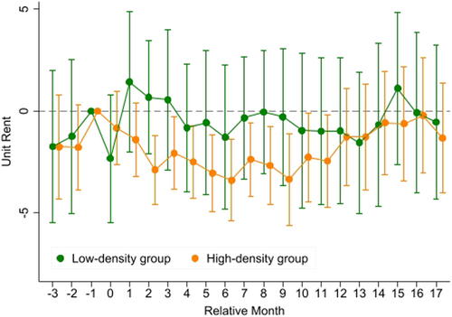
It is important to acknowledge that the results shown in Figure 5 may have limitations, particularly due to the staggered DID approach, which could introduce biases when estimating long-term effects.2 Nevertheless, the overall trends are consistent with our baseline results. This consistency strongly supports the conclusion that the decline in rental prices in high-density areas is primarily short-term and driven by the direct economic disruption resulting from reduced business activity and employment opportunities due to the lockdown. These findings further reinforce our view that the primary driver of rental price declines in high-density areas is a temporary economic slowdown in urban centers, which reduces local housing demand.
6.2 Migrant Population Outflow Would Contribute to the Change
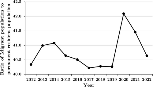
Our analysis suggests that the disproportionate impact of lockdown can be partly attributed to the cascading effects of disruption from the lockdown. Specifically, we propose a causal mechanism: lockdowns disrupt local economic activities, reduce employment opportunities, and subsequently trigger population outflows, particularly among migrant population. A decline in population density reduces housing demand and consequently lowers rental prices. We do not have neighborhood-level data on migrants and thus cannot estimate the causal effect of lockdowns on migrant outflow. However, below, we show supporting evidence for our proposed mechanism. As shown in Figure A1, the ratio of the migrant population to the permanent resident population in Shanghai declined at an accelerated pace in 2022. To further investigate this hypothesis, we employed data on the migrant population from Shanghai's 2021 and 2022 Statistical Yearbooks, which is shown in Table A4, alongside our original data, to examine the relationship between economic activity, population migration, and rental price dynamics during the lockdown period.
Using these data sets, we analyzed and visualized key metrics across the administrative districts of Shanghai, as depicted in Figure 6. The metrics include the density of company POIs (used as a proxy for business activity), the percentage change in the migrant population from 2021 to 2022, and the long-term percentage change in the migrant population between 2012 and 2022. The figure reveals that districts with higher company POI densities, such as Huangpu and Jing'an, experienced a more pronounced decline in migrant populations between 2021 and 2022. Furthermore, in many high-density districts, the short-term decline in migrant populations contrasts with their long-term upward trends from 2012 to 2022, indicating a significant departure likely driven by the economic disruptions caused by the lockdown. In contrast, districts with lower company POI densities experienced smaller population shifts and were less likely to deviate from their long-term population trends. These findings further support our proposed mechanism: the more significant rental price declines observed in high-density business districts can be attributed to temporary population outflows driven by economic disruptions. This is consistent with previous studies documenting the sensitivity of urban rental markets to economic shocks (e.g., Quigley and Rosenthal 2008; Glaeser et al. 2008). These results not only reinforce our main findings but also offer a broader perspective on the interplay between economic disruptions, population dynamics, and housing markets in the context of pandemic-induced lockdown.

7 Conclusion
This study offers a comprehensive analysis of the short-term and localized effects of lockdowns, providing a foundation for policymakers to consider appropriate responses to short-term crises. It specifically examines the impact of the COVID-19 lockdowns on rental prices in Shanghai, offering novel insights into the relationship between pandemic disruptions and urban housing markets. Drawing on detailed data from rental listings, company density, and lockdown orders, our analysis identifies two key findings. First, the lockdowns significantly impacted rental prices in high-density, business-oriented areas, causing a short-term decline of approximately 2.0%, with the effect peaking 2 months after the lockdowns. In contrast, suburban, low-density areas showed no statistically significant changes. This finding underscores the vulnerability of urban rental markets in economically concentrated regions, where rental demand is closely linked to local business activity and employment opportunities. Second, while rental prices in high-density areas initially declined, they demonstrated notable resilience, recovering to pre-pandemic levels within 12 months. This recovery highlights the adaptability of central urban rental markets, driven by structural demand for housing in business-dense areas and the eventual resumption of economic activity.
These findings contribute to the broader literature on the housing market impacts of the COVID-19 pandemic, emphasizing the heterogeneity of effects across urban and suburban areas. Consistent with prior research, these findings highlight the sensitivity of central business districts to economic shocks (e.g., Ramani and Bloom 2021; Ahrend et al. 2023; Beze and Thiel 2025). Future research could expand on this analysis by exploring how lockdown affects other aspects of the housing market.
Author Contributions
Yanpeng Jiang: conceptualization, data curation, formal analysis, funding acquisition, investigation, methodology, project administration, resources, software, supervision, validation, visualization, writing – original draft, writing – review and editing. Xiaochi Shen: conceptualization, data curation, formal analysis, funding acquisition, investigation, methodology, project administration, resources, software, supervision, validation, visualization, writing – original draft, writing – review and editing.
Acknowledgments
We would thank Nathan Schiff for helpful discussions and Wangyang Lai, Sai Luo, Helu Jiang, Xuebo Wang, and Zibin Huang for their comments.
Ethics Statement
Informed consent was not required for this study because this study does not contain any studies with human participants performed by any of the authors and are based on publicly available data.
Conflicts of Interest
The authors declare no conflicts of interest.
Endnotes
Appendix A: Supplementary tables and figures
See Tables A1–A4.
| Amap POI typecode | POI type | Observations |
|---|---|---|
| 170000 | Company enterprise; company enterprise; company enterprise | 5243 |
| 170100 | Company enterprise; well-known enterprise; well-known enterprise | 78 |
| 170200 | Company enterprise; company; company | 50,930 |
| 170201 | Company enterprise; company; advertising decoration | 2697 |
| 170202 | Company enterprise; company; construction company | 877 |
| 170203 | Company enterprise; company; pharmaceutical company | 522 |
| 170204 | Company enterprise; company; mechanical and electronic | 2056 |
| 170205 | Company enterprise; company; metallurgy and chemical industry | 800 |
| 170206 | Company enterprise; company; internet technology | 1616 |
| 170207 | Company enterprise; company; commercial trade | 1860 |
| 170208 | Company enterprise; company; telecommunications company | 187 |
| 170209 | Company enterprise; company; mining company | 5 |
| 170300 | Company enterprise; factory; factory | 1694 |
| 170400 | Companies and enterprises; agricultural, forestry, animal husbandry, and fishery bases; other agricultural, forestry, animal husbandry, and fishery bases | 1072 |
| 170401 | Companies and enterprises; agricultural, forestry, animal husbandry, and fishery bases; fisheries | 3 |
| 170402 | Companies and enterprises; agriculture, forestry, animal husbandry, and fishery bases; farms | 16 |
| 170403 | Companies and enterprises; agricultural, forestry, animal husbandry, and fishery bases; forest farms | 1 |
| 170404 | Companies and enterprises; agricultural, forestry, animal husbandry, and fishery bases; ranches | 0 |
| 170405 | Companies and enterprises; agriculture, forestry, animal husbandry, and fishery bases; poultry breeding bases | 3 |
| 170406 | Companies and enterprises; agriculture, forestry, animal husbandry, and fishery bases; vegetable bases | 10 |
| 170407 | Companies and enterprises; agriculture, forestry, animal husbandry, and fishery bases; fruit bases | 15 |
| 170408 | Companies and enterprises; agriculture, forestry, animal husbandry, and fishery bases; flower nursery bases | 14 |
| Total | 69,699 | |
- Note: This table provides a summary for company POI. Amap POI typecode and POI Type derived from AutoNavi Map's six-digit POI category codes.
- Abbreviation: POI, point-of-interest.
| (1) | |
|---|---|
| Variable | Number of risk areas |
| Panel A | |
| Distance to city center | −0.0565*** |
| (0.005) | |
| Observations | 1221 |
- Note: The table presents the coefficient and standard error regress the grids' number of risk areas and distance to city center. The regression results are estimated using robust standard errors. The predicted number of risk areas is used to refined control and treatment samples in Section 5.2.
- ***
- **
- * .
| Low-density group | High-density group | Total | |||
|---|---|---|---|---|---|
| Variables | Far from the treatment | Near the treatment | Far from the treatment | Near the treatment | |
| Rental price | |||||
| Number of rental listings | 6343 | 9460 | 2291 | 8432 | 26,526 |
| Unit rent (monthly, yuan/m2) | 91.71 (55.26) | 112.85 (57.57) | 106.40 (55.79) | 141.65 (61.58) | 116.40 (60.78) |
| House area (m2) | 67.01 (40.37) | 64.21 (41.04) | 70.08 (41.28) | 60.99 (41.58) | 64.36 (41.17) |
| Distance to city center (by community, km) | 23.07 (10.55) | 16.00 (7.95) | 18.61 (8.18) | 10.44 (5.98) | 16.15 (9.41) |
| Distance to subway station (by community, km) | 1.92 (3.13) | 1.02 (0.73) | 1.27 (1.47) | 0.70 (0.62) | 1.15 (1.75) |
- Note: The table presents summary statistics for rental prices and housing characteristics across reclassified groups for the spillover analysis in Section 5.3.
| Administrative district | Number of company POI | Area (km2) | 2022 Migrant population (million) | 2021 Migrant population (million) | 2012 Migrant population (million) |
|---|---|---|---|---|---|
| Huangpu District | 1848 | 20.46 | 0.2123 | 0.242 | 0.182 |
| Jing'an District | 2538 | 36.88 | 0.2204 | 0.245 | 0.0607 |
| Xuhui District | 3225 | 54.76 | 0.3147 | 0.3363 | 0.2941 |
| Changning District | 1756 | 38.3 | 0.2113 | 0.2218 | 0.1785 |
| Putuo District | 2460 | 54.83 | 0.3622 | 0.3651 | 0.3466 |
| Hongkou District | 1017 | 23.48 | 0.1802 | 0.1949 | 0.1865 |
| Yangpu District | 1627 | 60.73 | 0.2821 | 0.3057 | 0.2656 |
| Minhang District | 7187 | 370.75 | 1.1987 | 1.215 | 1.2602 |
| Jiading District | 8619 | 464.2 | 1.0398 | 1.0281 | 0.8808 |
| Baoshan District | 4836 | 270.99 | 0.8941 | 0.8915 | 0.8153 |
| Songjiang District | 7022 | 605.64 | 1.1079 | 1.1161 | 1.0483 |
| Pudong New Area | 12,567 | 1210.41 | 2.3659 | 2.4209 | 2.2284 |
| Fengxian District | 5991 | 687.39 | 0.559 | 0.5876 | 0.5715 |
| Qingpu District | 4449 | 670.14 | 0.6942 | 0.7316 | 0.6925 |
| Jinshan District | 3182 | 586.05 | 0.3069 | 0.2993 | 0.2364 |
- Note: The table presents summary statistics for migrant population and company POI across Shanghai administrative districts for the migrant population analysis in Section 6.2.
- Abbreviation: POI, point-of-interest.
See Figure A1.
Appendix B: Alternative Analysis Using Constructed Commuting Zones
This appendix presents an alternative approach from an earlier version of our study, which involves constructing commuting zones based on company POI and analyzing the impact of the lockdown on rents within these zones. While the results offer valuable insights, this approach is heavily reliant on parameter selection and is less generalizable than the model used in the main paper.
B.1 Commuting Zones
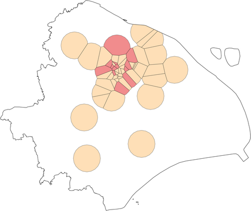
Commuting zones were constructed based on the concept of “employment clusters,” which are defined as geographic areas with a high concentration of enterprises. To identify these clusters, a customized 100 m 100 m grid was generated for Shanghai's digital map. Using corporate POI data, grids containing more than 20 enterprises were classified as “employment clusters,” leading to the identification of 55 clusters, which represent hubs of economic activity. On the basis of these clusters, commuting zones were delineated under the assumption that individuals working in an employment cluster are more likely to rent housing within the corresponding commuting zone. To partition Shanghai into distinct zones, centerlines were drawn between neighboring employment clusters. Furthermore, to better capture the rental market, the initial radius of commuting zones was extended to a maximum of 6 km, resulting in 55 zones. However, after accounting for sample distribution, only 54 zones were included in the final analysis, since one zone in the lower-left corner of Shanghai lacked sufficient rental listings, likely due to limited coverage by Beike.com. The commuting zones we defined are shown in Figure B1.
B.2 Lockdown-Related Employment Shock
Lockdown-related employment shock was defined based on the lockdown status of the employment clusters, following the example in Figure B2. Specifically, employment clusters were classified as “treated” if located within 200 m of a medium- or high-risk region under lockdown, where companies were required to close for at least 7 days. We hypothesize that such a lockdown may exert an effect on local employment. This disruption in economic activity consequently impacted local rental markets within the commuting zones surrounding these clusters. Consequently, commuting zones containing affected employment clusters were designated as “treatment zones,” while those without such disruptions were categorized as “control zones.”

B.3 Methodology
B.4 Key Finding
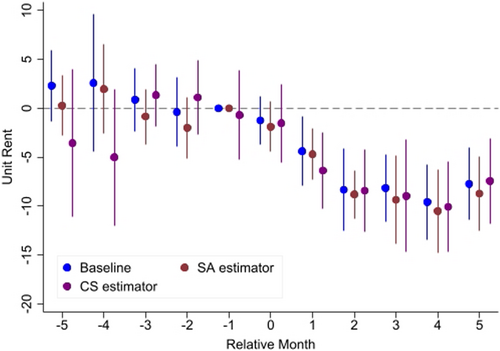
Employment-cluster lockdown significantly impacted rental prices within commuting zones. lockdown resulted in an average 5% decline in rental prices over a 6-month period following the intervention (Table B1). This decline was particularly pronounced in smaller apartments and properties located farther from central areas, likely due to reduced demand in less accessible locations and the greater mobility of lower-income tenants. Event-study analyses further confirmed these trends (Figure B3), showing a sharp and immediate decline in rental prices after the lockdown, with no significant pretreatment trends, thereby validating the parallel trends assumption. Rental price reductions persisted for several months before gradually stabilizing. Consistency across multiple estimation methods, such as Sun and Abraham (2021) and Callaway and Sant'Anna (2021), demonstrated the robustness of these findings and addressed concerns about potential biases introduced by staggered treatment effects. This finding aligns with the trend observed in our main analysis.
| (1) | |
|---|---|
| Variable | Unit rent |
| Panel A | |
| Treatment group staging impact | |
| 2-month effect | −3.533*** |
| (1.196) | |
| 4-month effect | −8.421*** |
| (2.162) | |
| 6-month effect | −8.898*** |
| (1.523) | |
| Panel B | |
| Average 6-month effect | −6.951 |
| (1.472) | |
| Mean of unit rent (before treatment) | 138.10 |
| Percentage of price decline | 5.03% |
| Observations | 60,498 |
| Control variables | Yes |
| Month fixed effect | Yes |
| Location fixed effect level | Commuting zone ∗ Neighborhood |
| Adjusted R2 | 0.491 |
- Note: The table presents the results of two-way fixed effects regression estimating the effects of employment-cluster lockdown on unit rental prices, with commuting zone ∗ neighborhood and month fixed effect. Standard errors are clustered at the commuting zone level.
- ***
- **
- * .
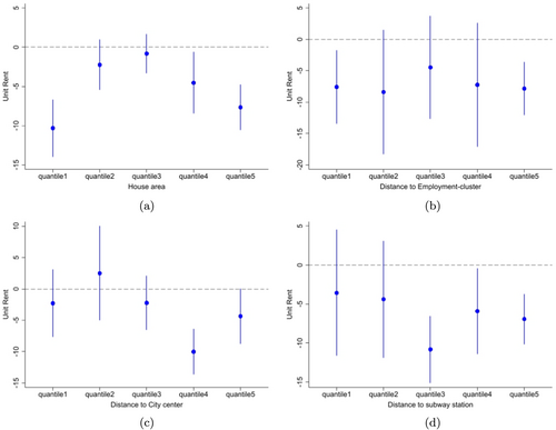
The analysis of heterogeneous effects, which is shown in Figure B4, reveals substantial variation in the impact of employment-cluster lockdown, depending on house attributes. Panel (a) of Figure B4 shows a hump-shaped trend, where the smallest residences experience the greatest decline in rental prices, reflecting the higher mobility and vulnerability of low-income tenants. Notably, larger properties also exhibit substantial price declines, suggesting that high-income households were not immune to the impact. Panel (b) indicates that the lockdown effect is relatively uniform across the commuting zones, supporting the hypothesis that employment-cluster lockdown broadly impact rental markets within these zones. Furthermore, Panels (c) and (d) reveal that properties farther from the city center and subway stations experienced more substantial price declines.
B.5 Discussion of the Advantage and Disadvantage of Commuting Zone Construction
The commuting zone construction provides several advantages and disadvantages when applied to the analysis of rental market dynamics during pandemic-induced lockdown:
Advantage 1: Comparability across zones. By defining commuting zones around employment clusters, this method establishes a consistent spatial framework that makes zones directly comparable. This enables a more systematic evaluation of localized effects, ensuring that each zone represents a cohesive economic and residential ecosystem.
Advantage 2: Enhanced heterogeneity analysis. Commuting zones allow for detailed exploration of heterogeneous effects, such as variations across housing attributes (e.g., house size, distance to city center, or proximity to subway stations). This granularity provides richer insights into the mechanisms driving rental price changes, particularly the interplay between housing characteristics and economic shocks.
Disadvantage 1: Parameter-dependent framework. The construction of commuting zones involves several arbitrary parameter choices, such as the size of the buffer zones (e.g., 6-km radius) and the thresholds for employment density (e.g., grids with at least 20 companies). These parameters introduce subjectivity and may lead to biases in the results, reducing the generalizability of the findings.
Disadvantage 2: Limited consideration of long commuting patterns. The commuting zone framework assumes that individuals primarily rent within their local zones. However, in a city like Shanghai, long commutes are common due to the extensive public transit network. This assumption may overlook rental market dynamics influenced by commuters renting farther from their workplaces.
Disadvantage 3: Increased complexity. Compared with the high-density versus low-density classification used in the main analysis, the commuting zone approach is more complex and computationally intensive.
Open Research
Data Availability Statement
Data associated with our study have not been deposited into a publicly available repository but will be made available on request.


