Environmental regulations and firm-level FDI: Evidence from China's 11th 5-year plan

1 INTRODUCTION

Since the early 1980s, China has sustained remarkably high rates of economic growth. This has coincided, however, with the rapid growth of energy, and pollution-intensive industries. Rodrigue et al. (2022), for instance, document that after China's WTO accession, production and trade from the Chinese manufacturing sector increased by 150% and 250%, but these increases came at a cost of 40% more sulfur dioxide (SO₂) emissions. The sharp increase in pollution contents associated with economic growth leads to unbalanced health gains for Chinese people: in the past two decades, life expectancy at birth only increased by 5.4 years, a modest gain relative to neighboring countries, such as South Korea (Ebenstein et al., 2015). Bombardini and Li (2020) further indicate that the increase in pollution contents significantly increases the infant mortality rate in China. In response to the growing deterioration of the environment, the Chinese government starts tightening its pollution regulations and aims at balancing economic growth and environmental sustainability. The more stringent environmental regulations deter the growth of dirty industries and force some firms to carry out production in countries with lax regulations, which is the so-called “pollution haven effect” (Taylor, 2004). In this paper, we intend to investigate the impact of environmental policy in China, the largest developing country, on firm-level outward foreign direct investment (OFDI). It will not only help us to understand the economic consequences of the environmental policy in the developing countries but also reveal the heterogeneous responses of different types of OFDI to the environmental policy, which sheds light on the inconclusive pollution haven literature.

OFDI refers to the phenomenon of home parent manufacturing firms that penetrate foreign markets through establishing affiliation there. From 1990 to 2006, the annual growth rate of world FDI flow is 17% (Irarrazabal et al., 2013). According to the World Investment Report, by 2006, 10% of world gross domestic product (GDP) is made up of the value added from multinational production. Meanwhile, as the largest developing country in the world, China's outward FDI flow accounts for 11.1% of global FDI flow and ranks second in the world by 2017. It is well-known that individual firms make their FDI decisions by balancing the tradeoff between saving variable trade costs and incurring irreversible FDI fixed costs. In response to a more stringent environmental regulation in the domestic country, firms may choose to carry out production in countries with lax environmental regulations through FDI to avoid paying expensive local emission taxes. As such, studying the pollution haven effect, especially the pollution haven effect through the lens of FDI responses, not only helps us to understand the determinants of environmental quality, but also uncovers the impact of environmental regulations on economic growth. To be more specific, first, the global efforts in reducing greenhouse gas emissions could be ineffective due to lax environmental regulations in some developing countries, which may attract global dirty FDI and cause a concentration of polluting industries there. Second, the concentration of polluting industries in some regions, especially in developing countries, brings health challenges, that is, the concentration of heavily polluting industries through FDI imposes a substantial health cost and therefore reduces the welfare level in these countries. Understanding the pollution haven effect through FDI is essential for countries to design their effective and cooperative environmental regulations.

Although the theoretical framework of the pollution haven effect has been well established, the literature that empirically examines the pollution haven effect finds inconclusive results (e.g., Chuang, 2014; Copeland et al., 2004; Hanna, 2010; Levinson, 1996; Levinson & Arik, 2008; Millimet & Roy, 2016). Hanna (2010), for instance, finds no evidence that heavily regulated American firms disproportionately increase production in developing countries. Similarly, Levinson (1996) uses a broad range of measures of environmental stringency and finds no systematical impact of environmental regulations on the location choices of manufacturing plants. Chuang (2014), in contrast, finds strong evidence that pollution industries in South Korea tend to invest more in countries with laxer environmental regulations. Levinson and Arik (2008) also claim that the industries that experience a significant increase in abatement costs in the United States increase their net imports from Canada and Mexico. Millimet and Roy (2016) further complete the findings of Levinson and Arik (2008) by addressing that more stringent environmental regulations in the United States attract more inbound FDI. To uncover the inconclusive literature, it is important to understand the heterogeneous impact of environmental policy, such as the 11th Five-Year Plan (FYP), on different types of FDI, for example, production-oriented or distribution-oriented FDI: if the prevalent FDI type is distribution-oriented in a particular country, a more stringent environmental policy will manifest a trivial pollution haven effect. As such, this paper contributes to the pollution haven literature by providing the heterogeneous impact of environmental regulations on different types of FDI, which explains the aforementioned inconclusive findings.

In this paper, we take advantage of China's 11th FYP to investigate the pollution haven effect through the channel of FDI. The plan aimed to reduce nationwide SO₂ emissions by 10% by the end of the year 2010. Unlike the proceeding FYPs, the 11th FYP handed down specific pollution reduction targets to each Chinese province. To achieve pollution reduction targets, provinces with higher pollution reduction targets have to establish more stringent environmental regulations. This provides both before-and-after and cross-province variations for identification, that is, firms located in provinces that face a higher reduction target have to face more stringent environmental regulations after 2006, which is the starting year of the 11th FYP.1 Therefore, we employ a difference-in-differences strategy to identify the impact, that is, provinces with more stringent regulations often set a higher emission tax (treated) than provinces with less stringent regulations (control).

Note that the emission tax we refer to here contains all explicit and implicit cost associated with emission. For instance, heavy polluters would be banned from getting government grants or loans or working on government contracts, which are implicit costs for emission.2

Specifically, we develop a simple model based on Helpman et al. to endogenize firm-level decisions on FDI, exporting, and serving only the domestic market. Each firm needs to pay a production cost and a tax for its emissions, which are byproducts of production (see Copeland & Taylor, 2003; Forslid et al., 2018). Firms balance the tradeoff between exporting and FDI, that is, exporting incurs an ice-berg transportation cost but saves the fixed start-up costs associated with FDI. When the emission tax rate increases in the home country (we assume a constant tax rate for emission in the foreign country throughout this paper), engaging in FDI not only saves the ice-berg transportation cost but also avoids paying a higher emission tax. Therefore, firms are more likely to engage in FDI in response to more stringent environmental regulations in their home country (pollution haven effect).3

To test the prediction of the model, we employ a data set that contains nationwide firm-level outward FDI from 1980 to 2012 and a firm-level production data set. We find that in provinces with a more stringent pollution reduction target, more firms start to engage in FDI. In addition, the FDI to export ratio, which is measured by the number of FDI firms over the number of exporters, also increases after the implementation of the environmental policy (in 2006). Furthermore, firm-level results indicate that: (1) firms are more likely to carry out FDI in developing countries rather than developed countries; (2) compared with distribution-oriented FDI, firms are more likely to engage in production-oriented FDI.4 These results are robust to a series of checks, that is, correcting for rare-events estimation bias, alleviating potential policy endogeneity, and adding various fixed effects. All findings provide positive support for the pollution haven effect: firms choose to carry out production-oriented FDI in developing countries for escaping from increased emission tax in the home country.

Beyond the aforementioned policy implications, this paper contributes to the literature in several dimensions. First, we examine the pollution haven effect in a developing country (i.e., China), which is significantly different from the existing research that studies the pollution haven effect by focusing on developed countries (Chuang, 2014; Hanna, 2010; Millimet & Roy, 2016). In particular, different from Hanna (2010) who finds no evidence that heavily regulated American firms disproportionably increase production in developing countries, we find clear evidence that heavily regulated Chinese firms are more likely to carry out FDI in developing countries. Second, our paper is a complement to Shi and Xu (2018), who find a negative effect of the 11th FYP on firm-level export participation probability and volumes, that is, according to Helpman et al., export and FDI are substitutable, and hence reductions in exports could partly be explained by more exporters switching to FDI during the 11th FYP period (e.g., Sun et al., 2020). Neglecting the impact of the 11th FYP on FDI would overestimate its negative effect on foreign sales. Third, our paper is also closely related to Cai et al. (2016) and Chen et al. (2019). In comparison with Cai et al. (2016), who examine the impact of environmental regulation on inbound FDI to China, we investigate the impact on China's outward FDI. Since most inbound FDI to China is from developed countries, Cai et al. (2016) actually examine the impact of environmental policy on FDI from developed countries. As a comparison, we investigate the influence of environmental policy on FDI from a developing country. Our work provides an explanation for Chen et al. (2019), who document that private firms engaged in FDI are less productive than state-owned enterprises (SOEs), but in the domestic market private firms are, on average, more efficient than SOEs: if the local government discriminates against private firms and imposes a higher emission tax on them (e.g., Huang, 2003, 2008), more private exporters will be forced to carry out FDI to escape from more stringent emission tax in the home country.5

In the next section, we introduce the background of the 11th FYP in China and describe the data we used. Section 3 develops a simple model to uncover the impact of environmental regulations on firm-level FDI participation decisions. Section 4 outlines the empirical strategy and reports the results. Finally, we conclude in Section 5.

2 BACKGROUND AND DATA DESCRIPTION

2.1 Background

To boost economic growth and improve environmental quality, China implements a series of countrywide FYPs to detail guidelines for economic and social development. The first FYP started from 1953 to 1957 and focused on economic growth. The 10th FYP was the first to include environmental development as a target, that is, by the end of 2005 the nationwide SO₂ emissions needed to be reduced by 10%. Unfortunately, since the 10th FYP set neither a clear SO₂ reduction target for each province nor a strict evaluation plan, the environmental goal had failed. In particular, nationwide aggregate SO₂ emissions increased around 30% from the year 2000 to the year 2005, which is the last year of the 10th FYP (see Shi & Xu, 2018).

To ease environmental deterioration, the 11th FYP during 2006–2010 handed down the national (SO₂) reduction goal to each province.6 Provincial goal attainment was evaluated using three specific criteria (State Council 2007c):7 (1) the quantitative goal itself and environmental quality; (2) the establishment and operation of three institutions: environmental goal setting of major pollutants, monitoring and the evaluation of environmental performance; (3) mitigation measures, including the installation and operation of pollutant removal facilities, the closure of inefficient factories, and so on. In addition, the tax rate for SO₂ emission dramatically increased (Xu et al., 2009), that is, the emission tax for SO₂ doubled during 2007–2010 compared with that during 2003–2005 and reached a price of $166 per ton of SO₂ emission.

Figure 1a shows the differential pollution reduction goals across provinces, and Figure 1b shows the geographic distribution of provinces that face a high- and low-reduction target, that is, provinces in the dark colors face a high-reduction target.8 Clearly, the pollution reduction targets exhibit significant regional variations. Hainan, for instance, faced a 0 reduction target (no target). In contrast, Beijing had to reduce the SO₂ emission by 20.4% by the end of 2010, which was a very stringent goal.

The different (SO₂) reduction goals across provinces imposed differential incentives in environment amelioration on local government. Shi and Xu (2018), for instance, document that provincial efforts/investments in removing air pollution increase reduction targets, that is, provinces that face a higher pollution reduction target tend to invest more in environment amelioration during the 11th FYP. Indeed, when we check the trend of aggregate SO₂ emissions across provinces in Figure 2, that is, the provinces with a high-reduction target (SO₂ reduction by more than ), and the ones with a low-reduction target (SO₂ reduction by less than ), we can observe a clear discrepancy across the two sets of provinces.

Figure 2 exhibits a sharper decline in the aggregate SO₂ emissions in high-reduction target provinces. Specifically, the total reduction of SO₂ emissions in provinces with a high-reduction target is approximately 4.67 times that in the provinces with a low-reduction target. The significant reduction in SO₂ emissions implies an effective environmental regulation, and we expect firms located in provinces with high pollution reduction targets to face more stringent environmental regulations, for example, a higher emission tax, more strict emission monitoring, and so on. These more stringent environmental regulations, in turn, increase firm-level production costs.

2.2 Data description

To empirically examine whether more stringent environmental policy encourages firm-level FDI activities, we employ two main data sets: (1) Firm-level FDI participation collected by the Ministry of Commerce of China, which covers the nationwide FDI activities and provides information about the FDI destination, purpose (distribution- or production-oriented), and so on; (2) the firm-level production data set, which provides firm-level production and financial information. More detailed information about these two data sets and summary statistics will be outlined below.

2.2.1 FDI data set

The nationwide data set contains firm-level FDI decisions collected by the Ministry of Commerce of China (MOC). Each Chinese FDI firm needs to report its detailed investment activities to the MOC since 1980. To invest abroad, each Chinese firm has to apply to the MOC to obtain approval and registration. During the application, each FDI firm must provide the MOC with the following information: firm name in China, the names of the firm's foreign subsidiaries, ownership (state- or private-owned), investment type (distribution- or production-oriented), the destination countries, and the amount of foreign investment. Once the FDI application is approved, the MOC will release to the public all the above-mentioned information but the amount of investment for business confidential concerns. Specifically, the MOC releases the following information about FDI firms: (1) name, (2) location, (3) the investment destination country, (4) ownership, (5) the names of foreign subsidiaries, (6) the FDI types, (7) the FDI starting date.

2.2.2 Annual Survey of Industrial Production (ASIP) data set

The ASIP data set provides firm-level production information for comprehensive SOEs and non-SOEs with annual sales exceeding 5 million RMB (roughly $770,000). During the sample period 2000–2008, these recorded enterprises account for more than of total industrial output and over of total industrial employment.9 The data set also reports comprehensive key financial variables, such as firm-level gross output, wage rate, capital stock, material input costs, employment, and so on. We follow Cai and Liu (2009) and clean the ASIP datasets by ruling out firms that report outliers. Specifically, firms report the total value of fixed assets is below RMB 10 million, the value of total sales is below RMB 10 million, the number of employees is below 8, total assets are below liquid assets and accumulated depreciation is below the net value of fixed assets.

We follow Chen et al. (2019) and carefully merge the FDI and ASIP data sets using firm names. Detailed information about the number of FDI firms, exporters, and matched firms is reported in Table 1.

Table 1. Trend of FDI number and share during 2000–2010

	2000	2001	2002	2003	2004	2005	2006	2007	2008	2009	2010
FDI starting	20	22	68	81	223	1002	1298	1429	1758	2542	3176
FDI accumulating	146	168	236	317	540	1542	2840	4269	6027	8569	11,745
Exporters	37,148	40,773	45,307	50,990	47,612	73,967	79,398	79,124	88,343	83,378	92,824
FDI/EXP ratio	0.0039	0.0041	0.0052	0.0062	0.0113	0.0208	0.0358	0.0540	0.0682	0.1028	0.1265
FDI starting(Treat)	15	18	38	52	180	741	930	1060	1337	1970	2414
FDI starting(Control)	5	4	30	29	43	261	368	369	421	572	762
FDI Accumulating(Treat)	102	120	158	210	390	1131	2061	3121	4458	6428	8842
FDI Accumulating(Control)	44	48	78	107	150	411	779	1148	1569	2141	2903
Merged FDI starting	5	6	9	30	75	366	452	479	453	–	–

• Note: Rows 1–2 report the trend of the new and accumulative number of FDIs (at firm-country-affiliate triplet); Row 3 shows the evolution path of the number of exporters, and Row 4 is the ratio of accumulative number of FDIs to the number of exporters, that is, ; Rows 5–8 report the trend of new and accumulative FDIs within treated and control regions, respectively.

In Table 1, we can observe a sharp increase in the number of firms that carry out FDI (at the firm-country-affiliate level) since 2000 (in Rows 1 and 2). In particular, Row 1 reports the newly started number of FDI firms each year, and Row 2 reports the accumulative number of FDI firms. Both Rows 1 and 2 exhibit a dramatic increase in years 2005,10 which is identical to the pattern documented by Chen et al. (2019). In addition, the matched number of FDI firms, which is reported in Row 9, also exhibits a similar trend as in Chen et al. (2019).11 In addition, we notice that although the number of exporters keep rising during the 2000–2010 period (Row 3), the number of FDI firms to the number of exporters ratio increased (Row 4).

Further, we divide all provinces into two categories: (1) treated provinces, which have more stringent reduction targets (reduce SO₂ emission by 5% or more); (2) control provinces, which have less stringent reduction targets (reduce SO₂ emission by less than 5%). Rows 5– 8 report the starting/accumulative number of FDIs for treated and control provinces, respectively. Although the number of new starting (accumulating) FDI firms increases in both treated and control provinces, the number of FDI firms increases faster in the treated provinces. To see this pattern clearly, we plot the trends of new starting (accumulating) number of FDI firms in treated and control provinces in Figure 3.12

The left panel of Figure 3 depicts the number of new FDI firms in treated and control provinces, and the right panel plots the number of accumulative FDI firms in treated and control provinces. Figure 3 exhibits a clearly divergent gap in the number of FDI firms between the treated and control provinces since the year 2005 (1 year before the implementation of the 11th FYP). As a comparison, we also depict the number of exporters in the treated and control provinces in Figure 4.

The left panel of Figure 4 depicts the trends of the number of exporters in the treated and control provinces, respectively. The treated and control provinces exhibit parallel trends in the number of exporters. The right panel of Figure 4 depicts the trend of the FDI to export ratio, computed by the number of FDI firms to the number of exporters, in treated and control provinces. It shows that the number of FDI firms to exporters ratio exhibits a clear divergent trend in the treated and control provinces. In sum, Figures 3 and 4 indicate two pieces of information: (1) the number of FDI firms increases faster in treated provinces, and the number of exporters increases at a similar speed in the treated and control provinces; (2) FDI to export ratio increases faster in treated provinces. These, in turn, may suggest that more stringent environmental policy encourages more firm-level FDI activities.

In the next section, we establish a simple model to explain the causal link between environmental policy and firm-level FDI activities, and the empirical analysis will be introduced in Section 4.

3 A SIMPLE MODEL

3.1 Demand

Both the home and foreign markets are assumed to manifest a monopolistic competition structure, that is, in either market, every active firm produces a heterogeneous variety. Consumers in both home and foreign markets have an identical CES preference as follows:

()

where  denotes the variety set in the home () and foreign countries (). is the consumed quantity of variety . denotes the constant elasticity of substitution between any two varieties. Note that since each firm produces a heterogeneous product, it obtains a certain degree of monopoly power in the market.

3.2 Supply

Each firm, in either the home or the foreign market, uses inputs to produce a single and heterogeneous variety, , to fit the market demand. We assume labor is the only input in production.

()

where and separately denote firm-level labor usage and productivity. We denote the wage level as , and the unit production cost can be written as . Due to the existence of the fixed cost, , the production exhibits an increasing return to scale feature (IRS).

3.4 Equilibrium

Denote , , and as productivity cutoffs for serving the domestic market, exporting, and FDI at the production cost, , respectively. The zero profit conditions for serving the domestic market, exporting, and FDI are characterized by Equations (3)–(5) as follows:

()

()

()

where is the revenue for firms with the cutoff productivity in the home country; denotes the export revenue for firms with cutoff productivity of exporting, , and measures the revenue through FDI for firms with cutoff productivity of FDI, . , , and are the fixed production cost in the domestic market, export, and FDI, respectively.15 To guarantee the equilibrium is well defined, we follow Helpman et al. and assume: (a) 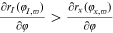; (b) .16 and represent the aggregate income in the home and foreign countries, respectively. Equations (3)–(5) define productivity cutoffs of staying in the market, starting export, and FDI, respectively. These cutoffs are also depicted in Figure 4.

In Figure 4, the three upward sloped lines , , and , denote the profit from serving the domestic market, serving the foreign market through exports, and serving the foreign market through FDI, respectively. Firms with productivity, , exit; firms will only serve the domestic market if their productivity is between ; firms will start to export if their productivity lies between ; and firms whose productivity is above engage in FDI.

For potential entrants, the expected profit is equal to the entry cost, which gives the free entry condition as follows:

()

Similar to Melitz and Redding (2015), with all the notations introduced above, the number of active firms can be expressed as:

()

where is the number of active firms, and is the number of potential entrants. is the total labor supply in the home country. and denote the average revenue earned by active firms and the average fixed cost paid by all firms, respectively. In particular,

where and denote the proportion of firms engaged in export and FDI, respectively. So far, we have completed characterizing the equilibrium in the economy, that is, active firms make optimal choice based on Equations (3)–(5); potential entrants make entry decisions according to Equation (6); labor market clearing condition is summarized by Equation (7).

3.5 Environmental regulations and FDI decisions

In this section, we investigate the impact of environmental regulations on firm-level FDI decisions.17 Suppose the environmental regulations become more stringent, that is, increase to , and hence . According to Equations (3)–(5), we have18

()

Inequalities (8) indicate that when the emission tax rate increases, the cutoff productivity in the domestic market and exporting increases. In contrast, the cutoff productivity of engaging in FDI decreases.19 We also show the impact of more stringent environmental regulations on these cutoffs in the following Figure 5.

In Figure 5, the red-dash lines, , and separately denote profit from serving the domestic market and exporting, after the increase in the emission tax rate. Since we assume the emission tax only increases in the domestic market, the profit from FDI does not change, that is, and overlap. Note that an increase in emission tax rate increases firm-level production cost, , and hence the domestic and exporting profit falls at each productivity level. As a result, the domestic and exporting profit curve shifted to the right-hand side related to the original ones. The intuition is quite straightforward: when the production costs, which contain the emission costs, increase in the domestic market, firms have a stronger incentive to shift their production to foreign countries to avoid paying the increasing emission tax. As such, some firms switch from exporting to FDI and the FDI productivity cutoff falls.

Our simple model indicates that when the emission tax rate increases, the cutoff productivity of engaging in FDI will decrease while the productivity cutoffs for exporting and in the domestic market increase. Therefore, among all active firms, the proportion of FDI firms increases in the emission tax rate. Formally, we have the following proposition:

Proposition 1.In response to a more stringent environmental regulation (increase in ), firms are more likely to engage in FDI to escape from paying the higher emission tax.

In the next section, we will take advantage of China's 11th FYP as a quasi-natural experiment to test proposition 1.

4 EMPIRICAL RESULTS

As illustrated in Section 2, China's 11th FYP motivated heterogeneous environmental regulations across provinces, that is, provinces that had been imposed a higher SO₂ reduction target tend to set a more stringent environmental regulations. We make use of the variation in pollution reduction targets, which measures the variation of environmental regulations, across provinces and the before-and-after change to examine the impact of environmental regulation on firms' FDI decisions. In particular, our empirical analysis consists two parts: we first investigate the impact of environmental regulations on the aggregate province-level FDI numbers (FDI to exporter ratios); second, using a matched sample, we examine the influence of environmental regulations on firm-level FDI participation decision.

4.1 Province-level regression

Our baseline estimation employs a DIDs specification to link the heterogeneous reduction targets in SO₂ emissions across provinces and FDI activities. In Figures 2 and 3, we have shown that the trends of FDI numbers and FDI to export ratio diverges for low- and high-reduction targets provinces, that is, provinces with a higher reduction target in SO₂ emissions, experience faster growth in both FDI numbers and FDI to export ratio than provinces with a lower reduction target. For more rigorous empirical examination, we specify a DID estimation in Equation (9) and examine the heterogeneous responses of FDI activities in different provinces to the implementation of the 11th FYP.

()

where the subscript and separately denote province and year. represents the province-level variables of interest, that is, aggregate province-level number of FDI firms, number o FDI firms to the number of exporters ratio, which is measured by , and the number of FDI firms to the number of nonexporters ratio, which is measured by , respectively. measures the SO₂ reduction target in province during the 11th FYP period.20 equals 1 after 2006 which is the starting year of the 11th FYP, and equals 0 before 2006. denotes province-level controls, including province-level highway freight value, education expenditure, inward FDI, research expenditure, internet coverage, and GDP. Table 2 reports the impact of environmental regulations on the province-level number of FDI firms.

Table 2. DID results for number of FDI Firms—province-level

	(1)	(2)	(3)	(4)	(5)
	0.444***	0.466***	0.477***	0.402***	0.386***
	(3.05)	(3.12)	(3.19)	(2.73)	(2.66)
		−0.010	−0.109	−0.225***	−0.408***
		(−0.66)	(−1.27)	(−2.63)	(−3.99)
			0.071	0.027	−0.357***
			(1.17)	(0.44)	(−3.22)
				0.156***	0.099**
				(4.00)	(2.11)
					−0.036
					(−0.40)
					−0.025
					(−0.32)
					0.480***
					(3.81)
Province FE	Yes	Yes	Yes	Yes	Yes
Year FE	Yes	Yes	Yes	Yes	Yes
obs	390	390	390	390	390
Adj	0.818	0.818	0.818	0.825	0.832

• Note: Columns 1–5 report the estimated impact of the 11th FYP on the province-level number of FDI firms by adding more province-level controls. All standard errors have been clustered at the province level and the t value is reported in the parenthesis. ***, **, and * separately denote significance at the 99%, and 95%, and 90% levels.

Columns 1–4 in Table 2 add more and more controls. The results indicate that the coefficient on is always positive and statistically significant. This implies that in provinces that are set more stringent environmental regulations, the number of FDI firms increases faster than that in provinces with less stringent environmental regulations. In addition, highway freight value and education expenditure exhibit a negative impact on FDI activities, that is, the former captures the transportation efficiency and the latter measures the skilled labor ratio, and hence, the negative effects suggest that more efficient inland transportation and better local education discourage FDI. In contrast, inward FDI and local GDP manifest a positive and significant effect on FDI, that is, the inward FDI may generate information spillovers and hence encourages outward FDI, while a higher local GDP captures the relative higher efficiency in production which also encourages FDI.

Table 3 reports the impact of the 11th FYP on the province-level number of FDI to the number of exporters/non-exporter ratios, respectively.

Table 3. DID results for FDI ratio—province-level

	(1)	(2)	(3)	(4)	(5)	(6)
	0.326***	0.286**	0.460***	0.369**	0.307**	0.211
	(2.85)	(2.53)	(3.06)	(2.48)	(2.09)	(1.44)
		−0.359***		−0.407***		−0.381***
		(−4.40)		(−3.79)		(−3.62)
		−0.141		−0.374**		−0.280*
		(−1.19)		(−2.41)		(−1.84)
		−0.009		0.000		−0.005
		(−0.24)		(0.00)		(−0.11)
		0.092		0.155		0.153
		(1.25)		(1.60)		(1.60)
		−0.094		−0.071		−0.108
		(−1.56)		(−0.90)		(−1.38)
		0.259**		0.411***		0.295**
		(2.23)		(2.70)		(1.97)
Province FE	Yes	Yes	Yes	Yes		Yes
Year FE	Yes	Yes	Yes	Yes		Yes
Obs	390	390	390	390	390	390
Adj	0.938	0.941	0.875	0.882	0.854	0.861

• Note: Columns 1–2 report the impact of the 11th FYP on accumulative FDI to exporter ratio; Columns 3 and 4 report the impact of the 11th FYP on the new FDI to export ratio; Columns 5 and 6 report the new FDI to nonexporter ratio. All standard errors have been clustered at the province level and the t value is reported in the parenthesis. ***, **, and * separately denote significance at the 99%, 95%, and 90% levels.

Columns 1 and 2 in Table 3 report the impact of 11th FYP on the accumulative FDI to export ratio; Columns 3 and 4 report the impact of 11th FYP on the new FDI to export ratio, and Columns 5 and 6 report the impact of 11th FYP on FDI to nonexporting firm ratio. The results indicate that in provinces that are set more stringent environmental targets, the ratios measured by accumulative FDI firms to exporters, new FDI firms to exporters, and new FDI firms to nonexporters are all increasing faster than that in provinces with less stringent environmental targets. All these results are consistent with the predictions of our model.

4.2 Heterogeneous effects

To further check the differential FDI trends in high- and low-reduction target provinces are not driven by confounding factors, we estimate the following specification and examine the heterogeneous effects:

()

where denotes the total number of firms that are located in province and conduct FDI in country . is a dummy variable, which takes a value of 1 if country is a developing country, otherwise, it takes a value of 0.21 If the sharp increase in the number of FDI firms is driven by the more stringent environmental regulations, we should expect a positive and significant : firms are more likely to conduct FDI in developing countries where the environmental regulation is laxer to escape from a higher emission tax in the domestic country (see Eskeland & Harrison, 2013; Levinson & Arik, 2008). The results are reported in Table 4 below.

Table 4. DDD results—different FDI destinations

	(1)	(2)	(3)	(4)	(5)
	0.387*	0.455**	0.497**	0.457**	0.461**
	(1.68)	(1.97)	(2.16)	(2.02)	(2.04)
	0.176	0.036	0.003	−0.007	−0.026
	(0.95)	(0.18)	(0.01)	(−0.04)	(−0.14)
		0.021**	−0.192***	−0.303***	−0.447***
		(2.24)	(−2.74)	(−4.13)	(−5.07)
			0.161***	0.089	−0.081
			(3.06)	(1.64)	(−0.90)
				0.176***	0.124**
				(4.53)	(2.60)
					−0.036
					(−0.40)
					−0.038
					(−0.53)
					0.173
					(1.58)
Prov-Dest FE	Yes	Yes	Yes	Yes	Yes
Dest-Year FE	Yes	Yes	Yes	Yes	Yes
Obs	390	390	390	390	390
Adj	0.759	0.761	0.764	0.771	0.832

• Note: , where is an FDI destination dummy. is the FDI destination is a developing country, otherwise, it takes a value of zero. All standard errors have been clustered at the province level and the t value is reported in the parenthesis. ***, **, and * separately denote significance at the 99%, 95%, and 90% levels.

The results in Columns 1–4 of Table 4 show that the coefficient on the triple interaction term, , is always positive and statistically significant. This implies that the increasing trend in the number of FDI firms is mainly driven by firms that conduct FDI in developing countries rather than in developed countries. This finding is consistent with the pollution haven hypothesis and provides support to our model. To further test the model's predictions, we conduct a firm-level analysis.

4.3 Firm-level regression

4.3.1 DID Estimation

To examine whether the 11th FYP plays a key role in the firm-level decision of engaging in FDI, we consider the following empirical specification:22

()

where represents the FDI decision of firm that is located in province , which takes a value of 1 if firm engages in FDI in year , and 0 otherwise. denotes firm-level controls, such as productivity, capital to labor ratio, size, R&D investment, and export intensity. and capture province and year fixed effects, and we cluster all standard errors at the province level. The results are reported in Table 5 below:

Table 5. The impact of emission reduction targets on FDI participation–firm-level DIDs

	Linear Probit				PPML	Rare Event
	(1)	(2)	(3)	(4)	(5)	(6)	(7)
	0.034**	0.041**	0.045**	0.044**	0.332**	0.489***	0.489***
	(2.30)	(2.43)	(2.01)	(2.20)	(2.19)	(3.23)	(3.20)
		0.020***	0.030***	0.036**	0.299***	0.100	0.240***
		(2.88)	(2.08)	(2.05)	(2.91)	(1.12)	(4.43)
		0.017**	0.027***	0.029***	0.378***	0.296***	0.248***
		(2.40)	(2.76)	(2.84)	(12.57)	(9.93)	(8.96)
		0.051**	0.067***	0.068***	0.708***	0.603***	0.611***
		(2.58)	(2.74)	(2.75)	(20.02)	(22.55)	(23.80)
		0.118**	0.134**	0.133***	0.745***	0.986***	0.615***
		(1.99)	(2.18)	(2.79)	(7.90)	(12.34)	(7.25)
		0.074**	0.108***	0.108***	1.011***	0.863***	0.981***
		(2.33)	(2.80)	(2.79)	9.94	(15.17)	(11.25)
Province FE	Yes	Yes	Yes	Yes	Yes	Yes	Yes
Year FE	Yes	Yes	Yes	No	Yes	Yes	Yes
Industry FE	No	No	Yes	No	Yes	Yes	Yes
Ownership FE	No	No	Yes	No	Yes	No	No
Owner-Year FE	No	No	No	Yes	Yes	No	No
Indus-Year FE	No	No	No	Yes	Yes	No	No
Obs	2,471,481	1,882,639	1,298,861	1,298,858	471,710	1,180,210	1,298,863
Adj	0.010	0.023	0.028	0.028	0.181	0.270	–

• Note: Columns 1–4 report the impact of the 11th 5-Year Plan on firm-level FDI activities by controlling for different fixed effects. All coefficients have been multiplied by 100 in Columns 1–4. Column 5 reports the PPML results. Columns 6 and 7 report the rare event logit results by using cloglog and relogit, respectively. All standard errors have been clustered at the industry level and the t value is reported in the parenthesis. ***, **, and * separately denote significance at the 99%, 95%, and 90% levels.

Column 1 of Table 5 only includes the interaction term, , and fixed effects. In Columns 2–4 we contain all firm-level controls and various sets of fixed effects to conduct a linear probability estimation. Specifically, in Column 2 we control for province and year fixed effects; Column 3 further controls for industry and ownership fixed effects. This is to mitigate the concern that different industries and firms with different ownerships may manifest heterogeneous trends in conducting FDI, which would cause a potential bias in our estimation. Column 4 controls for the province, ownership-year, and industry-year fixed effects which pin down differential trends across ownerships and industries. In Column 5, instead of using a linear probability model, we estimate specification (11) using a high-dimension Poisson regression. Furthermore, to alleviate the concerns that our sample exhibits the feature of rare events that occur infrequently, standard econometric methods such as logit and probit would underestimate the probability of rare events (see King & Zeng, 2001, 2002). We follow Tian and Yu (2020) and use a complementary log-log model to address this issue in Column 6.23 In Column 7 we correct rear event bias following King and Zeng (2001, 2002), that is, we first estimate the finite sample bias of the coefficient bias(), to obtain the bias-corrected estimate , where denotes the coefficient obtained from the conventional logistic estimates. The coefficients on are all positive and statistically significant in all columns, which implies that firms located in provinces with more stringent environmental regulations are more likely to start FDI.

4.3.2 Difference-in-difference-in-differences (DDD) estimation

Further, we conduct two DDD regressions to examine: (1) what countries, for example, developing or developed ones, attract more FDIs from China? (2) what types of FDI, production-oriented or distribution-oriented FDI, increases faster during the 11th FYP period, that is, distribution-oriented outward FDI refers to firms that penetrate foreign markets through wholesale trade affiliates that resell exportable goods.

()

()

where in Equations (12) and (13) the subscript , , denote firm, province and year, respectively. denotes FDI destination country in Equation (12), and FDI type in Equation (13). and are dummies. if the FDI destination country is a developing country, and takes a value of 0 otherwise. takes a value of 1 for production-oriented FDI and equals 0 for distribution-oriented FDI. , , and separately capture the province-destination/province-type, destination-year/type-year, and province-year fixed effects.

Columns 1–3 in Table 6 report the results from linear probability estimation, and Column 4 reports the result from high-dimension Poisson probability estimation. The coefficient on the triple interaction term, , is always positive and statistically significant. This suggests that during the 11th FYP period, firms in high-reduction target provinces are more likely to start FDI in developing countries relative to developed countries. This provides firm-level evidence that firms carry out FDI in developing countries, which often have lax environmental regulations, to escape from more stringent environmental regulations.

Table 6. Firm-level DDD results: FDI destinations

	Linear Prob			PPML
	(1)	(2)	(3)	(4)
	0.132**	0.162***	0.160**	1.113***
	(6.14)	(4.32)	(2.30)	(11.77)
	0.008*	0.016	0.018	0.081
	(1.65)	(1.63)	(1.59)	(0.68)
	0.013**	0.016***	0.016***	0.195***
	(2.51)	(2.72)	(2.75)	(7.75)
	0.044***	0.046***	0.047***	0.603***
	(2.66)	(2.67)	(2.70)	(12.55)
	0.079**	0.077**	0.076**	0.510***
	(2.08)	(2.03)	(2.02)	(3.69)
	0.047**	0.061**	0.062**	0.818***
	(2.13)	(2.32)	(2.33)	(4.95)
Prov-year FE	Yes	Yes	Yes	Yes
Dest-year FE	Yes	Yes	Yes	Yes
Prov-dest FE	Yes	Yes	Yes	Yes
Ownership FE	No	Yes	No	No
Industry FE	No	Yes	No	No
Indus-year FE	No	No	Yes	No
Owner-year FE	No	No	Yes	No
Obs	1,298,805	1,298,805	1,298,805	460,004
Adj	0.365	0.365	0.365	0.436

• Note: Columns 1–3 report the impact of the 11th 5-Year Plan on firm-level FDI activities in developing countries by controlling for different fixed effects. , where is the FDI destination is a developing country, otherwise, it takes a value of zero. All coefficients have been multiplied by 100 in Columns 1–3. Column 4 reports the PPML results. All standard errors have been clustered at industry level and the t-value is reported in the parenthesis. ***, **, and * separately denote significance at the 99%, 95%, and 90% levels.

Similarly, Columns 1–3 in Table 7 reports the result from linear probability estimation, and Column 4 reports the result from high-dimension Poisson probability estimation.24 The coefficient on the triple interaction term, , is always positive and statistically significant. This indicates that during the 11th FYP period, firms in provinces with more stringent environmental regulations are more likely to participate in production-oriented FDI than distribution-oriented FDI. Combining with the finding in Table 6, these results imply that in response to more stringent regulations, more firms offshore production in developing countries. If escaping from more stringent environmental regulations in the domestic country is not the main concern, we would expect the distribution-oriented FDI to increase at a similar rate as the production-oriented FDI.

Table 7. Firm-level DDD results—FDI types

	Linear Prob			PPML
	(1)	(2)	(3)	(4)
	0.270**	0.269**	0.269**	1.261**
	(2.57)	(2.56)	(2.55)	(2.13)
	0.034**	0.040**	0.042**	0.169**
	(2.33)	(2.38)	(2.21)	(2.13)
	0.024**	0.031**	0.031**	0.279***
	(2.50)	(2.49)	(2.52)	(10.38)
	0.076**	0.081**	0.083**	0.743***
	(2.52)	(2.53)	(2.53)	(26.23)
	0.118**	0.108*	0.104*	0.481***
	(1.84)	(1.76)	(1.71)	(6.56)
	0.096**	0.124**	0.124**	0.974***
	(2.07)	(2.39)	(2.38)	(12.13)
Prov-year FE	Yes	Yes	Yes	Yes
Prod-year FE	Yes	Yes	Yes	Yes
Prov-prod FE	Yes	Yes	Yes	Yes
Ownership FE	No	Yes	No	No
Industry FE	No	Yes	No	No
Indus-year FE	No	No	Yes	No
Owner-year FE	No	No	Yes	No
Obs	1,298,805	1,298,805	1,298,805	459,136
Adj	0.315	0.315	0.316	0.374

• Note: Columns 1–3 report the impact of the 11th 5-Year Plan on firm-level FDI activities by controlling for different fixed effects. , where is the FDI purpose is for production, and it takes a value of zero if the FDI purpose is for providing sales service. All coefficients have been multiplied by 100 in Columns 1–3. Column 4 reports the PPML results. All standard errors have been clustered at the industry level and the t value is reported in the parenthesis. ***, **, and * separately denote significance at the 99%, 95%, and 90% levels.

4.4 Robustness checks

In this section, we conduct a series checks to verify the robustness of our results.

4.4.1 Endogeneity

In the above specifications, we take advantage of China's 11th FYP to investigate the impact of environmental regulations on FDI activities. However, after the plan established a pollution reduction target for the entire country, each province negotiated with the central government for their individual reduction target.25 It is possible that the central government strategically assigns some provinces a higher pollution reduction target according to provincial characteristics, and endogeneity arises because of confounding factors. To mitigate the endogeneity concern, we follow Shi and Xu (2018) and use the ventilation coefficient, which is the product of wind speed and mixing height, as an IV for provincial pollution targets. The ventilation coefficient largely determines the rate at which pollution disperses over space. That is, the variation in pollution concentration across times and space is effectively exogenous as it is largely determined by weather systems. We leverage variation in ventilation coefficients across space to capture the exogenous variation in environmental concerns of the central government.26 We re-estimate the firm-level and province-level regressions with the ventilation coefficient IV and the results are reported in Tables 8 and 9, respectively. In particular, Columns 1–3 in Table 8 report the firm-level IV results by adding different fixed effects; in Column 4 we further add the county-level minimum wage to alleviate the concern that the increase in firm-level FDI results from an increase in labor wage, rather than increased emission tax;27 In Columns 5 and 6, we repeat the DDD specification by instrumenting the DID and DDD with and (or ), respectively.

Table 8. Robustness bhecks–Firm-level 2SLS

	(1)	(2)	(3)	(4)	(5)	(6)
					0.210**	0.451***
					3.01	(6.04)
	0.161**	0.160**	0.163***	0.164***
	(2.50)	(2.49)	(3.18)	(3.18)
	0.023***	0.032***	0.037***	0.037***	0.014	0.042**
	(2.84)	(3.08)	(3.29)	(3.29)	(1.51)	(2.22)
	0.021***	0.027***	0.028***	0.028***	0.013**	0.031**
	(5.83)	(6.03)	(6.01)	(5.98)	(2.55)	(2.56)
	0.061***	0.066***	0.067***	0.067***	0.045**	0.082**
	(6.32)	(6.39)	(6.43)	(6.41)	(2.74)	(2.53)
	0.139***	0.133**	0.133***	0.133***	0.078**	0.104
	(5.60)	(5.37)	(5.26)	(5.26)	(2.12)	(1.70)
	0.093***	0.107**	0.108**	0.108***	0.042	0.124**
	(2.74)	(3.03)	(3.04)	(3.03)	1.34	(2.38)
				0.006
				(0.18)
Province FE	Yes	Yes	Yes	Yes	No	No
Year FE	Yes	Yes	No	No	No	No
Industry FE	No	Yes	No	No	No	No
Ownership FE	No	Yes	No	No	No	No
Owner-year FE	No	No	Yes	Yes	No	No
Indus-year FE	No	No	Yes	Yes	No	No
Prov-year FE	No	No	No	No	Yes	Yes
Dest-year FE	No	No	No	No	Yes	Yes
Prov-dest FE	No	No	No	No	Yes	Yes
Cragg–Donald F	6.9e+05	6.9e+05	6.8e+05	6.8e+05	1.1e+06	2.03+06
KP-rk LM	22.18	22.09	20.17	20.25	12.41	12.02
Obs	1,298,863	1,298,863	1,298,8860	1,298,860	1,298,855	1,299,171
Adj	0.014	0.014	0.014	0.014	0.009	0.023

• Note: Columns 1–4 report the 2SLS results using pre-period province-level ventilation coefficient as an IV for treatment and control for different fixed effects; Column 4 further add the county-level minimum wage to avoid changes in labor cost deviate firm-level OFDI activities; shows the most results from the most flexible specifications; Columns 5 and 6 separately report the DDD results for firms OFDI to a different destination and for a different purpose. All standard errors have been clustered at the industry level and the t-value is reported in the parenthesis. ***, **, and * separately denote significance at the 99%, 95%, and 90% levels.

Table 9. Robustness checks–Province-level 2SLS

	(1)	(2)	(3)	(4)	(5)	(6)
						1.556**
						(1.97)
	1.000***	0.993***	1.000***	0.691*	0.711**	−0.965
	(2.83)	(2.81)	(2.83)	(1.94)	(2.03)	(−1.34)
		−0.022	−0.133	−0.234***	−0.410***	−0.311***
		(−1.27)	(−1.57)	(−2.70)	(−3.98)	(−3.45)
			0.084	0.037	−0.340***	−0.136
			(1.35)	(0.60)	(−3.02)	(−1.30)
				0.146***	0.091*	0.111**
				(3.60)	(1.92)	(2.42)
					−0.043	0.015
					(−0.47)	(0.17)
					−0.032	−0.047
					(−0.41)	(−0.68)
					0.475***	0.236*
					(3.74)	(1.89)
Province FE	Yes	Yes	Yes	Yes	Yes	No
Year FE	Yes	Yes	Yes	Yes	Yes	No
Prov-dest FE	No	No	No	No	No	Yes
Dest-year FE	No	No	No	No	No	Yes
Cragg–Donald F	76.73	79.34	79.12	72.43	71.99	23.87
KP-rk LM	70.29	72.41	72.41	67.51	67.65	49.61
Obs	390	390	390	390	390	390
Adj	0.681	0.877	0.890	0.942	0.860	0.993

• Note: Columns 1–5 report the estimated impact of the 11th FYP on the province-level number of FDI firms by adding more province-level controls. In all columns, we instrument province-level reduction targets with province-level ventilation coefficients. All standard errors have been clustered at the province level and the t-value is reported in the parenthesis. ***, **, and * separately denote significance at the 99%, 95%, and 90% levels.

We first notice that all our OLS results remain, that is, firms that in provinces facing more stringent environmental regulations are more likely to conduct FDI; further, firms tend to conduct production-oriented FDI in developing countries. Second, the magnitude of the coefficients on DID and DDD significantly increases from previous settings. This may suggest that when the central government sets heterogeneous reduction targets across provinces, it also takes into account the local economic growth, that is, the reduction targets could be slightly lower in provinces with a lot of FDI and exporting firms because of stringent environmental regulations impede economic growth. Third, we report the Cragg–Donald F statistics at the bottom of Table 8, which are sufficiently large. This implies that our IV does not suffer from weak IV issues.

In Table 9, we repeat the province-level regression by constructing the same set of IVs. Again, all results remain.

4.4.2 Expectation effect

The 10th FYP had set a pollution reduction target for the whole country (2000–2005), but no evaluation scheme was clearly defined.28 This resulted in the failure of the pollution reduction goal during the 10th FYP. As such, firms may expect a more stringent environmental regulation in the 11th FYP, and make corresponding responses even before the implementation of the 11th FYP. To address this concern, we estimate the following specification:

()

where all variables have the same meaning as before. and are dummies, which take the value of 1 in years 2004 and 2005, respectively. If the coefficient of or is positive, the expectation effect exists. The results are reported in Column 1 of Table 10. The results show that both and are positive and significant ( is statistically insignificant), this implies that firms expected more stringent environmental regulations in the 11th FYP, and started to carry out FDI in 2005.

Table 10. Robustness–flexible settings

	(1)	(2)	(3)	(4)
	0.077***		0.049***	0.229**
	(3.30)		(3.08)	(2.45)
		−0.094
		(−0.94)
		−0.014
		(−1.38)
		−0.018
		(−1.52)
	0.031	0.021
	(1.29)	(1.50)
	0.069***	0.059***
	(3.30)	(2.88)
		0.054***
		(2.63)
		0.080***
		(4.08)
	0.021***	0.021***	0.021***	0.020***
	(2.71)	(2.87)	(2.95)	(4.06)
	0.022***	0.022***	0.022***	0.017***
	(11.00)	(10.92)	(10.98)	(11.88)
	0.065***	0.065***	0.065***	0.053***
	(28.53)	(16.81)	(16.81)	(17.87)
	0.135**	0.135***	0.135***	0.114***
	(17.99)	(11.12)	(11.13)	(11.96)
	0.100**	0.818***	0.101***	0.080***
	(13.12)	(8.82)	8.82	(8.98)
			−0.029**
			−2.45
			−0.040***
			−5.64
			0.037***
			5.52
Province FE	Yes	Yes	Yes	Yes
Year FE	Yes	Yes	Yes	Yes
Industry FE	NO	No	No	No
Ownership FE	No	No	No	No
Obs	1,298,805	460,004	1,298,805	1,882,639
Adj	0.015	0.023	0.015	0.019

• Note: Column 1 reports the pre-cautious effects; Column 2 shows the results from the most flexible specifications; Column 3 reports the results after controlling for some province-year characteristics; In Column 4, if the province SO₂ reduction tariff is above 5%, otherwise . All standard errors have been clustered at industry level and the t value is reported in the parenthesis. ***, **, and * separately denote significance at the 99%, 95%, and 90% levels.

4.4.3 Flexible estimation

In Column 2 of Table 10, we adopt a very flexible specification, in which we replace the interaction with a series of interaction terms between and year dummies, that is, . The estimated coefficients for these interactions are uniformly insignificant for years before 2005. The interactions turn to be positive and significant since the year 2005. This result suggests that firm-level FDI participation increased since 2005, which is 1 year before the 11th FYP, and kept rising in the following years.

4.4.4 Province-level controls

In Column 3, we re-estimate specification (11) and control for a series of province-year variables, that is, province-year level education expenditure, inward FDI, and investments. This will alleviate the concern that some province-year-level confounding factors may bias our benchmark estimation.

4.4.5 Binary treatment definition

In Column 4, we follow Callaway et al. (2020) and define for province whose reduction target is equal to or above , and otherwise. The results show that firms located in high-reduction target regions are more likely to participate in FDI in the 11th FYP.

4.4.6 The mechanism

Notice that different industries are heterogeneous in their pollution intensities, and hence will be affected differentially during the 11th FYP.29 Similar to Shi and Xu (2018), we construct industry-level SO₂ emission intensities during 2000–2005, , we then estimate the following specification:

()

Equation (15) examines the heterogeneous impact of the 11th FYP on heavy- and light-pollution industries. If the mechanism we addressed early is correct, we would expect a positive and statistically significant : that is, compared with firms that belong to the light-pollution industries, firms in heavy-pollution industries have a larger incentive to carry out FDI to avoid paying the expensive emission tax domestically. The results are reported in Table 11.

Table 11. Mechanism check—Firm-level

	OLS			IV
	(1)	(2)	(3)	(4)	(5)	(6)
	0.019**			0.019*
	(2.27)			(1.77)
	0.028	0.018	0.064***	0.28	0.136**	0.257***
	(1.38)	(1.49)	(4.39)	(1.38)	(2.30)	(5.22)
	0.012*	0.033**	−0.003	0.012*	0.034***	1.66e−06
	(1.78)	(2.42)	(−0.41)	(1.78)	(3.02)	(0.02)
	0.028***	0.024**	0.031**	0.028***	0.024***	0.032***
	(10.23)	(2.36)	(2.27)	(10.83)	(6.97)	(6.97)
	0.054***	0.053**	0.057**	0.054***	0.053***	0.032***
	(12.86)	(2.28)	(2.16)	(12.86)	(9.26)	(8.27)
	0.147***	0.159**	0.133**	0.054***	0.159***	0.133***
	(10.11)	(2.00)	(2.06)	(12.86)	(7.66)	(6.56)
	0.099***	0.135***	0.078**	0.099***	0.133***	0.076***
	(7.38)	(2.67)	(2.26)	(7.38)	(5.91)	(4.75)
Industry-year FE	Yes	Yes	Yes	Yes	Yes	Yes
Prov-industry FE	Yes	Yes	Yes	Yes	Yes	Yes
Cragg–Donald F				1.9e+06	2.7e+05	1.8e+05
KP-rk LM				1197.45	375.19	735.95
Obs	937,338	446,842	487,953	937,338	487,953	446,842
Adj	0.022	0.019	0.022	0.010	0.010	0.039

• Note: Columns 1–3 report the estimated impact of the 11th FYP on firm-level FDI participation decisions by dividing firms into heavy- and light-pollution industries. Columns 4–6 repeat the estimation by using 2SLS. In particular, Columns 1 and 3 report the DDD results; Columns 2 and 4 present the results for light-pollution industries, and Columns 3 and 6 report the results for heavy-pollution industries. All standard errors have been clustered at the province level and the t value is reported in the parenthesis. ***, **, and * separately denote significance at the 99%, 95%, and 90% levels.

All results in Table 11 indicate that firms that belong to more heavily polluting industries are more likely to conduct FDI than firms in clean industries.

5 CONCLUSION

In this paper, we investigate the impact of environmental regulations on firms' FDI participation. We first establish a simple model to incorporate emission tax into firm-level production function. The productivity cutoffs of engaging in FDI, exporting, and serving the domestic market rely critically on emission tax: when the emission tax rate in the domestic market increases, the productivity cutoff of conducting FDI decreases, but productivity cutoffs for exporting and serving the domestic market increases. This implies that more firms will engage in FDI to escape from more stringent environmental regulations.

We next take advantage of the 11th FYP in China, which specifies different pollution reduction targets across provinces and examine the heterogeneous responses of firm-level FDI participation to this policy. Specifically, we investigate the impact of environmental regulations on FDI participation at both the province level and firm level by employing a DID approach. The province-level results indicate that the total number of FDI firms in provinces with more stringent reduction targets increases faster, as well as the number of FDI firms to the number of exporters ratio. Furthermore, the firm-level analysis implies that (1) firms that are located in provinces with more stringent environmental regulations are more likely to participate in FDI during the period of the 11th FYP; (2) firms in provinces with more stringent environmental regulations are more likely to carry out FDI in developing countries rather than developed countries; (3) after 2006, firms in provinces with more stringent environmental regulations are more likely to engage in production-oriented FDI rather than distribution-oriented FDI. These results are consistent with the prediction of the model and provide support to the emission-tax-escaping channel, that is, local firms choose to engage in FDI to escape from the increasing emission tax. Our results are robust to a series of checks.

This study generates important policy implications: although more stringent environmental regulations discourage firm-level production (in the domestic market) and exporting (e.g., Shi & Xu, 2018), they encourage firm-level FDI participation, which increases firm-level profitability in the long run.

AUTHOR CONTRIBUTIONS

Yong Tan: Conceptualization, project administration, writing review and editing. Qing Shi: writing-original draft. Siyuan Xuan: data sorting and dealing. Guang Yang: plot figures.

CONFLICT OF INTEREST

The authors declare that there are no conflicts of interest.

ETHICS STATEMENT

None declared.

REFERENCES

- 1 The emission tax, like the emission charge for SO2 is set at the national level, but provinces that face a higher reduction target have a higher incentive to monitor firm-level pollution emissions, and force heavy polluters to install abatement equipment (see Xu, 2011). This increases firm-level implicit emission tax.
- 2 We refer to readers to OECD (2009) for a more detailed discussion about implicit emission tax.
- 3 Sun et al. (2020) document a very similar idea as us. They show that a higher trade cost will force more firms to switch from exporting to FDI.
- 4 Distribution-oriented FDI refers to building overseas business offices to explore the foreign market, promote sales, and serve customers in the hosting countries (Hanson et al., 2001; Tian & Yu, 2020).
- 5 Huang (2003) points out that the Chinese government systematically favors SOE financially and legally. As such, SOEs in China have better access to finance, which makes it easier for SOE to comply with stricter environmental regulations than private firms (Hering & Poncet, 2014). Shi and Xu (2018) also find the trivial impact of the environmental regulations (the 11th FYP) on exports of SOEs, although the impact on private and foreign-owned firms is significant.
- 6 After the nationwide (SO2 reduction) goal was established, the provinces negotiated with the central government for their share of the burden. The China State Council issued a document named Reply to Pollution Control Plan during the 11th Five-Year plan in 2006, which handed down the national goal to pollution reduction by the provincial vice presidents (State Environment Protection Administration, 2006).
- 7 The State Council 2007c can be found: http://www.gov.cn/zwgk/2007-11/23/content_813617.htm.
- 8 All provinces that face an SO2 reduction target of more than 5% are treated as a high-reduction target province, while provinces that face a reduction target of less than 5% are treated as a low reduction target province.
- 9 The period 2000–2008 contains the pre- and post-period of the 11th FYP, and hence provide us an appropriate sample period to investigate the impact of the 11th FYP on firm's OFDI activities.
- 10 The 11th FYP starts from 2006, and the dramatic increase in the number of OFDI firms may reflect the precaution effects. We thank an anonymous referee to mention the year 2005 issue.
- 11 The matched number of FDI firms is nontrivially lower than that reported in Chen et al. (2019). This is because Chen et al. (2019) add other sources of FDI information, that is, they merged small- and median-sized FDI firms in Zhejiang province to the sample, which is unavailable to us.
- 12 To plot Figure 2, we sum up the aggregate number of FDI firms in all treated and control provinces (in each year), respectively. The left panel of Figure 2 plots the trend of the new starting number of FDI firms, and the right panel reports the trend of accumulating number of FDI firms.
- 13 More productive firms use less input, labor, to produce certain units of output, and hence generate lower emissions. This is called the technical effect in Antweiler et al. (2001). Also, DeSousa et al. (2015) find that production pollution increases in the intermediates used. Although we do not explicitly assume intermediate usage in the production process, we could extend the production of final products in two steps: each firm first produces intermediates using labor, and second, assemble a series of intermediates to produce the final products. The assumption here captures the idea that more productive firms are cleaner than less productive firms.
- 14 Recall that labor is the only input in production, and hence the cost, including emission tax, is paid in labor. For firm with productivity
, producing 1 unit output requires
unit labor and generates
unit emission, and hence the production cost is
.
. - 15 We assume emissions only arise in the production process, and hence the fixed cost part does not contain an emission tax. We argue that we can relax this assumption, and allow the fixed cost to take the form
,
,  , and
, and  .
. - 16 Assumption (1) implies that FDI revenue (so as profit) increases faster in productivity than exporting revenue (profit); Assumption (2) indicates that the fixed cost is higher for carrying out FDI than that associated with exporting. The two assumptions guarantee the single-crossing property of the FDI revenue (profit) and exporting revenue (profit) curves.
- 17 According to a suggestion from an anonymous referee, we can introduce a transaction platform for SO2 emissions, in which each firm freely buy or sell SO2 emission quotas, and the emission tax rate will be endogenously determined by the equilibrium condition in the emission transaction platform. However, this extension is under the assumption that each province has its own emission transaction platform. As such, the emission quotas cannot be traded across provinces. The proof in the appendix shows that a more stringent environmental regulation will translate into a higher emission tax rate,
. - 18 The detailed proof is available in the appendix.
- 19 In the appendix, we show in detail that
. - 20
is a continuous variable in our benchmark regression. As a robustness check, we also follow the classical DID setting and divide provinces into treated and control groups, that is, provinces that needed to reduce SO2 emission by 5% or more are treated, and provinces that needed to reduce SO2 emission by less than 5% are control (see Shi & Xu, 2018).
- 21 Developing countries are defined by the World Bank as countries with per-capita GNIs below $9760 in 2007 are classified as developing countries. We also use definition of developing country by IMF, and all results remain.
- 22 Recall that we have matched FDI and ASIP data sets. All the following firm-level analysis are conducted using the matched sample. Note that since the ASIP data set spans from 2000 to 2008, the firm-level analysis only is conducted using the data during 2000–2008 which is a shorter span than the province-level analysis.
- 23 The complementary log-log regression allows faster convergence toward rare events (see Chen et al., 2019).
- 24 In addition to control for province-year, type-year and province-type fixed effects, Column 2 further control for ownership fixed effects, and Column 3 further control for industry-year and ownership year fixed effects.
- 25 For individual province's reduction target, the Central State Council issued a document named Reply to Pollution Control Plan during the 11th Five-Year-Plan in 2006, which handed down the national goal to pollution reduction by the provincial vice president.
- 26 We thank an anonymous referee who suggests us to clarify the mechanism through which the ventilation coefficient affects province-level reduction targets.
- 27 If labor wage increases differentially across provinces during the same period, our previous results only reveal the impact of increased production costs (e.g., labor costs) on firm-level OFDI decision. As such, we collect the minimum wage data from each county of China during the same period, and use it to control for differential trends in labor costs across regions.
- 28 Xu (2011), for instance, states that in the 10th FYP, only several principles were stated, including holding local government leaders accountable, and linking environmental goal attainment with the leaders' performance evaluation.
- 29 We appreciate two anonymous referees to point out this issue.