Reliable local dynamics in the brain across sessions are revealed by whole-brain modeling of resting state activity
Funding information Consejo Nacional de Investigaciones Científicas y Técnicas, Grant/Award Number: PhD Grant ; Danish National Research Foundation, Grant/Award Number: DNRF117; German Science Foundation, Grant/Award Numbers: DFG KU 3322/1-1, SFB 936/C7; H2020 European Research Council, Grant/Award Numbers: Advanced Grant DYSTRUCTURE (n. 295129), ERC Consolidator Grant CAREGIVING (n.615539), ERC-2016-StG-Self-Control-677804; Jacobs Foundation, Grant/Award Number: JRF 2016-2018; Spanish Ministry of Economy and Competitiveness, Grant/Award Number: PSI2013-42091-P; National Scientific and Technical Research Council
Abstract
Resting state fMRI is a tool for studying the functional organization of the human brain. Ongoing brain activity at “rest” is highly dynamic, but procedures such as correlation or independent component analysis treat functional connectivity (FC) as if, theoretically, it is stationary and therefore the fluctuations observed in FC are thought as noise. Consequently, FC is not usually used as a single-subject level marker and it is limited to group studies. Here we develop an imaging-based technique capable of reliably portraying information of local dynamics at a single-subject level by using a whole-brain model of ongoing dynamics that estimates a local parameter, which reflects if each brain region presents stable, asynchronous or transitory oscillations. Using 50 longitudinal resting-state sessions of one single subject and single resting-state sessions from a group of 50 participants we demonstrate that brain dynamics can be quantified consistently with respect to group dynamics using a scanning time of 20 min. We show that brain hubs are closer to a transition point between synchronous and asynchronous oscillatory dynamics and that dynamics in frontal areas have larger heterogeneity in its values compared to other lobules. Nevertheless, frontal regions and hubs showed higher consistency within the same subject while the inter-session variability found in primary visual and motor areas was only as high as the one found across subjects. The framework presented here can be used to study functional brain dynamics at group and, more importantly, at individual level, opening new avenues for possible clinical applications.
1 INTRODUCTION
Ongoing resting state activity is a powerful tool that enables a detailed exploration of the brain's functional organization at multiple spatial scales (Deco, Jirsa, & McIntosh, 2011; Singer, 2013). At the group level, many studies have addressed the intrinsic functional architecture of the healthy brain (e.g., Damoiseaux et al., 2006; Honey, Thivierge, & Sporns, 2010) while many others have focused on the differences between control participants and patients suffering from a wide variety of brain disorders, such as schizophrenia (Damaraju et al., 2014; Lynall et al., 2010), Parkinson's Disease (Göttlich et al., 2013) and autism (Jones et al., 2010). Although these studies uncovered important information about the functional principles of brain activity, few of them have focused on consistent methods applied at a single-subject level and in ways that information is relevant when used in the clinical environment (but see Mueller et al., 2013; Laumann et al., 2015).
This represents a major issue given the well-known large anatomical and functional variability across individuals (Frost & Goebel, 2012; Pannunzi et al., 2017). Moreover, functional variability is also expected within a single subject depending on many factors such as the state of the subject and environmental noise (Mueller et al., 2013). A reliable single-subject analysis of brain dynamics should then yield stable and reproducible results across different sessions (Fiecas et al., 2013; Zuo & Xing, 2014), and be sensitive enough to show between-groups contrast (Castellanos, Di Martino, Craddock, Mehta, & Milham, 2013; Ferreira & Busatto, 2013). Previous studies that analyzed the functional connectivity (FC) of the brain using a correlation matrix or using more advanced statistical techniques such as independent component analysis (ICA) (Damoiseaux et al., 2006; reviewed in Fox & Raichle, 2007) hypothesized that functional connectivity is constant over time, although it is now becoming clear that even at rest, there are dynamical processes worth considering (Hutchison, Womelsdorf, Gati, Everling, & Menon, 2013). Conversely, numerous studies have postulated that brain dynamics are essential to explain both health and disease, placing fluctuation of phase synchronization as one of the main features required to understand how integration and segregation arise and modulate brain states (Tognoli & Kelso, 2014). For this reason, some groups have proposed that functional connectivity dynamics (FCD) have to be taken into account to develop FC-related metrics that properly reflect temporal aspects of brain function (Calhoun, Miller, Pearlson, & Adalı, 2014; Deco et al., 2014; Deco, Tononi, Boly, & Kringelbach, 2015; Hansen, Battaglia, Spiegler, Deco, & Jirsa, 2015).
In this context, whole-brain computational models have been used as powerful tools to understand the relation between structural and functional brain connectivity by linking brain function with its physiological underpinnings (Ponce-Alvarez, He, Hagmann, & Deco, 2015; Deco et al., 2015; Kringelbach et al., 2015). In contrast to conventional resting state analyses, studies based on brain models allow the exploration of brain dynamics (Deco et al., 2014; Deco & Kringelbach, 2016) both in health and disease (Cabral et al., 2013). Recent studies used a novel whole-brain modeling technique to simulate brain dynamics estimating local parameters containing information about the oscillatory nature of a given region (Deco, Kringelbach, Jirsa, & Ritter, 2017; Jobst et al., 2017). These previous works have shown modeling to be a powerful tool for the analysis of brain dynamics for the description of brain states and the changes during disease. Nevertheless, they did not deepen in the between-session and between-subjects consistency of these modeling-based parameters. In this work, we make a progress and use this model to develop a multimodal processing method to provide new insights about brain function at a single-subject level as well as to estimate consistency of local dynamics and to explore the minimum scan length and number of sessions required to have a robust estimation.
We also demonstrated that the metrics derived from local modeled dynamics provide a powerful framework that can be used to quantify localized brain activity consistently across participants and sessions. Using 50 longitudinal resting state (rs-fMRI) sessions from a single subject and by comparing the within-subject consistency to that estimated using 50 recordings from different participants we searched for the optimal number of sessions required for accurately estimate these parameters. Finally, we studied which brain regions exhibited higher consistency within subjects compared with the consistency across subjects.
2 MATERIALS AND METHODS
2.1 Conceptual considerations of whole-brain computational modeling
Modeling of brain signals classically have been organized into two main model families (a) noise-based and (b) oscillatory based (Cabral, Kringelbach, & Deco, 2017). To reconcile noise-based approaches with models based on oscillators, Hopf bifurcation based models have been proposed. Based on the normal form of a Hopf bifurcation (Freyer et al. 2011, 2012), the behavior of the signal generator abruptly change after trespassing the critical value of one or more parameters; in particular, a Hopf bifurcation occurs when a system characterized by a stable fixed point loses its stability by exhibiting oscillations. As such, this model allows transitions between asynchronous noise activity and oscillations, thus making it a good candidate to reproduce empirical data as observed with EEG, MEG, or fMRI (Cabral, Kringelbach, & Deco, 2017).
In this work, we developed and applied a supercritical Hopf model (Deco, Kringelbach, et al., 2017; Jobst et al., 2017) that uses functional and structural connectivity (SC) information to simulate whole-brain activity. Importantly, this model has been applied to disease (Saenger et al., 2017) and altered states of consciousness (Jobst et al., 2017), revealing important characteristics of the resting brain architecture. As shown in Figure 1, the model uses brain dynamics from fMRI data as well as the SC from diffusion weighted imaging (DWI) data to construct an interconnected network (Figure 1a). In this network, each node (brain region) presents supercritical Hopf bifurcation dynamics (Marsden & McCracken, 2012) that depending on the value of its bifurcation parameter (BP) reflect if the region behaves either in a noisy asynchronous or stable oscillatory manner (Figure 1b). A negative BP means that the node is working as a noise generator, while a positive BP generates stable oscillatory dynamics. Thus, when a node's BP is away from zero, it is expected to not respond to the environmental conditions. Lastly, nodes that exhibit a BP around zero can be understood as flexible systems on the edge of a bifurcation, capable of changing their information profile depending on physiological demands. Therefore, a “flexible brain” at rest is expected to have a global mean of the bifurcation parameters centered around zero in order to rapidly adapt to environmental or internal demands (Deco, Kringelbach, et al., 2017). An in-depth mathematical explanation of this model and its optimization can be found in the Supporting Information. The fine-tuning of each BP allows the description of how each brain region operates as a signal generator, engaged in a network determined partially (but not exclusively) by the SC data. A model with the right set of BPs allowed us to simulate brain signals, matching dynamical properties of the brain. Therefore, we named the full set of BPs as dynamical core (DynCore) of the brain (Deco, Kringelbach, et al., 2017).
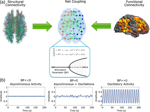
The model is fitted to the empirical data (blood oxygen level dependent [BOLD] signal) of each subject using the DynCore and an extrinsic global scaling factor G that determines the impact of the SC on brain dynamics. In the fitting process, we iterate over G, to find (at each step of G) a single DynCore by using a gradient descendent algorithm to fit nodal spectral distributions between empirical and simulated BOLD signals. Then, we use a similarity score to automatically find the optimal G and DynCore that allows simulating best the empirical data through the model. The similarity score we developed unifies static and dynamical properties of the brain system into a single metric, making it feasible to detect the subject's DynCore (see Supporting Information for more details). We then used this optimal DynCore as a functional descriptor of the brain and analyzed its consistency across subjects and sessions.
2.2 Participants
Fifty-one participants were recruited in total from which one participant volunteered to be included in the longitudinal part of the study in which she was scanned 50 times over the course of 6 months (female, aged 29). The remaining fifty participants (all female, mean age 25, SD = 3.27, range: 18–32) underwent scanning with the same MRI sequences only once.
The study was approved by the local ethics committee (Charité University Clinic, Berlin). All participants gave written consent and were asked whether they ever had a psychiatric disease during recruitment. Other medical and neurological disorders were also reasons for exclusion. None of the participants showed structural abnormalities in the MRI scans.
2.3 fMRI data collection
Images were collected on a 3 T Magnetom Trio MRI scanner system (Siemens Medical Systems, Erlangen, Germany) using a 12-channel radiofrequency head coil. Structural images were obtained using a three-dimensional T1-weighted magnetization-prepared gradient-echo sequence (MPRAGE) based on the ADNI protocol (www.adni-info.org) (repetition time (TR) = 2,500 ms; echo time (TE) = 4.77 ms; TI = 1,100 ms, acquisition matrix = 256 × 256 × 192 mm3, flip angle = 7°; bandwidth = 140 Hz/pixel, 1 × 1 × 1 mm3 voxel size). Functional images were collected using a T2*-weighted echo planar imaging (EPI) sequence sensitive to BOLD contrast (TR = 2000 ms, TE = 30 ms, image matrix = 64 × 64, FOV = 216 × 216 × 129 mm3, flip angle = 80°, bandwidth = 2042 Hz/pixel, voxel size 3 × 3 × 3 mm3, 36 axial slices using parallel imaging [GRAPPA] with an acceleration factor of 2, 5:08 min duration).
2.3.1 fMRI data preprocessing
The first 10 volumes were discarded to allow the magnetization to approach a dynamic equilibrium. Data preprocessing, including slice timing, head motion correction (the least squares approach and a 6-parameter spatial transformation), linear trend removal, and spatial normalization to the Montreal Neurological Institute (MNI) template (resampling voxel size of 3 × 3 × 3 mm3), were conducted using the SPM5 and data processing assistant for resting-state fMRI (DPARSF, Chao-Gan & Yu-Feng, 2010). A spatial filter of 4 mm full-width at half maximum (FWHM) was used. One fMRI recording with head motion above 2 mm of maximal translation (in any direction of x, y, or z) and more than 1.0° of rotation throughout the course of scanning was excluded. To reduce spurious fluctuations in functional connectivity (Laumann et al., 2016) motion-induced noise was regressed out (three rigid body rotations and translations, as well as their first three temporal derivatives, resulting in 24 motion regressors) from the functional data using the least squares and retaining the residuals.
The data were parcellated into regions of interest (ROIs) using the automated anatomical labeling (AAL) atlas (Tzourio-Mazoyer et al., 2002). Each recording was represented by 90 nodes with 140 time points for each node. fMRI data were temporally band-pass filtered (0.01–0.25 Hz) to reduce low-frequency drift and high-frequency respiratory and cardiac noise (Biswal, Zerrin Yetkin, Haughton, & Hyde, 1995). Additionally, given that the whole-brain computational uses the relationship between the energy distribution in a narrow frequency band and a wide frequency band for the optimization, we estimated narrow band time signals, filtered in the range 0.04–0.07 Hz, by using a sixth order Butterworth band-pass filter (Cordes et al., 2001). This frequency band has been mapped to the gray matter and it has been shown to be more reliable and functionally relevant than other frequency bands (Achard, Salvador, Whitcher, Suckling, & Bullmore, 2006; Biswal et al., 1995; Buckner et al., 2009; Glerean, Salmi, Lahnakoski, Jääskeläinen, & Sams, 2012).
2.4 DWI data used on the model
We used an averaged structural connectome obtained using DWI in 16 different healthy right-handed participants (11 men and 5 women, mean age: 24.75 ± 2.54), recruited through the online recruitment system at Aarhus University. In this study, participants with psychiatric or neurological disorders (or a history thereof) were excluded from participation. The MRI data was recorded in a single session on a 3 T Siemens Skyra scanner at CFIN, Aarhus University, Denmark. Structural T1-Weighted MRI scans were adquired with an isotropic voxel size of 1 mm3; a reconstructed matrix size of 256 × 256 pixels, TE of 3.8 and TR of 2,300 ms.
The DWI data were collected using a TR = 9,000 ms, TE = 84 ms, flip angle = 90°, reconstructed matrix size of 106 × 106, voxel size of 1.98 × 1.98 mm with slice thickness of 2 mm and a bandwidth of 1,745 Hz/Px. The data were recorded with 62 optimal nonlinear diffusion gradient directions at b = 1,500 s/mm2. One non-diffusion weighted image (b = 0) per 10 diffusion-weighted images was acquired. Additionally, the DWI images were recorded with different phase encoding directions. One set was collected applying anterior to posterior phase encoding direction and the second one was acquired in the opposite direction. To co-register the DWI image to the T1-weighted structural image, we used the linear registration tool from the FSL toolbox (www.fMRIb.ox.ac.uk/fsl, FMRIB, Oxford) (Jenkinson, Bannister, Brady, & Smith, 2002). We co-registered the T1-weighted image to the T1 template of ICBM152 in MNI space. The resulting transformations were concatenated and inversed and further applied to warp the AAL template (Tzourio-Mazoyer et al., 2002) from MNI space to the DWI native space, where we preserved the discrete labeling values by applying interpolation using nearest-neighbor method. Accordingly, brain parcellation was conducted in each participant's native space. The acquired DWI data were used to generate the SC maps for each participant. The two recorded datasets were processed, each with different phase encoding to optimize signal in difficult regions. To construct these SC maps we applied a three-step process. First, we defined the regions of the whole-brain network with the AAL template as used in the functional MRI data. Second, we used probabilistic tractography to estimate the connections between nodes in the whole-brain network (i.e., edges). Finally, the data were averaged across participants.
In accordance with the procedure applied for analyzing the rs-fMRI data, the AAL template was used to parcellate the entire brain into AAL90. In order to co-register the b0 image in diffusion MRI space to the T1-weighted structural image and then to the T1 template of ICBM152 in MNI space (Collins, Neelin, Peters, & Evans, 1994), we used the FLIRT tool from the FSL toolbox (www.fMRIb.ox.ac.uk/fsl, FMRIB, Oxford). We concatenated and inversed the two transformation matrices from the described co-registration steps and applied them correspondingly to warp the AAL templates (Tzourio-Mazoyer et al., 2002) from MNI space to the diffusion MRI native space.
2.5 Whole-brain model as a processing approach
 (1)
(1)Using this processing approach, we were able to identify an optimal DynCore of single fMRI recordings and also of group of recordings, obtaining a mean DynCore by concatenating multiple recordings before the frequency filtering (as in Deco, Kringelbach, et al., 2017).
Finally, DynCores with a KSDist larger than 0.3 or a Fitting smaller than 0.25 were discarded as we considered the rs-fMRI recording to be noisy and unsuitable for the model to further generate acceptable simulations of brain dynamics. In this work, more than 4,000 simulations were generated with a rejection rate of around 10%.
2.5.1 Normalization of BPs
The main problem of using raw bifurcation parameters to study brain dynamics at a single subject level is that, depending on Gi, BPs can have very different ranges (Figure 2a). Therefore, each set of BPs[G opt] has values that cannot be directly compared between different datasets, irrespective of whether they come from the same or different subjects.
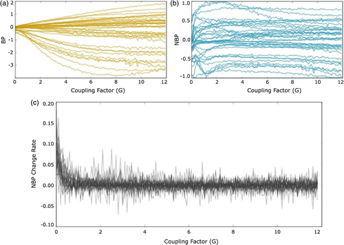
 ) (Figure 2c), making comparisons between subjects and sessions possible. To this aim we took each
BPsi (set of BPs for a given
Gi) and split them in two subsets, one containing all the positive values (
pBPi) and another with all negative ones (
nBPi). To obtain the normalized bifurcation parameter set (
NBPsi) we divided
pBPi and
nBPi by the largest absolute value on that subset. This procedure is given by Equations 2, 3, and 4,
 (2)
(2) (3)
(3) (4)
(4)2.6 Combinatorial analysis
An important issue we aimed to address is the minimum scanning time required to obtain stable results, that is to say, the point at which the error to a reliable measurement does not diminish as we add more scanning time. For this, we implemented a combinatorial analysis in which we gradually increased the number of concatenated resting state recordings. The analysis consisted of: (a) Obtaining the DynCore for each single fMRI recording, (b) Concatenate 50 random sets of two fMRI recordings, (c) Repeating this while increasing number of concatenated recordings until using 20 recordings by steps of 1, (d) For each of these steps (from 1 to 20) we obtained two types of DynCores, a set 50 raw DynCores and a single median DynCore that was calculated by computing the median of the NBPs for each brain region.
This combinatorial analysis allowed us to simulate the effect of having different scanning times and therefore to explore consistency as scanning time is progressively increased.
2.6.1 Optimal scanning time estimation
We used the Euclidean distance (square root of the sum of squared nodal-wise differences) to the reference mean DynCore (the one obtained by concatenating all the recordings) to study how the consistency changes as more resting state functional magnetic resonance (rs-fMRI) data is used in the calculation of the DynCore. In the first place we looked for an optimal scanning time using the error to the median DynCore of each number of sessions (from 1 to 20). The median DynCore was obtained by keeping the median for each region's NBP.
2.6.2 Within-subject and between-subjects reliability comparison
In the clinical environment, each patient usually is scanned only once, which makes difficult to calculate a median DynCore across different sessions. To analyze this, situation we studied Euclidean distances between each raw DynCore (without using the median of each BP) and the reference mean DynCore. We then compared within-subject intersession variability with between-subject variability using the DynCores and its distance to the references DynCore and analyzed how this distance changes as more rs-fMRI sessions are used in the estimation of the DynCore through the model.
2.6.3 Region-wise consistency assessment
 (5)
(5) (6)
(6)This metric represents how many times the between-subject variability of a node is larger than that found within-subject.
3 RESULTS
3.1 Normalization of bifurcation parameters
To show the effect of the normalization, we started by exploring the behavior of the intrinsic BPs across the extrinsic coupling factor G. Figure 2a illustrates how raw BPs depend on G in a nonlinear way, which makes comparison across subjects and sessions difficult. In contrast, when the normalization is performed, these values become stabilized for G > 2 (Figure 2b), allowing the comparison across subjects and sessions. Figure 2c depicts the change rate of the mean BP for 50 different recordings of the same subject, demonstrating the enhanced reliability of this normalization procedure for G > 2.
3.2 Within-subject consistency of normalized bifurcation parameters
An important goal is to demonstrate that the DynCore is a measure that reliably captures properties of brain dynamics, which can be used to compare both local and global brain dynamics within the same subject. To this aim we compared the results of two different within-subject processing pipelines using the same data. We obtained a single DynCore concatenating all 50 rs-fMRI sessions from the same subject, which is plotted in Figure 3 as a gray-dotted line and represents the optimal baseline DynCore. Furthermore, we obtained a set of 1,000 DynCores by using the combinatorial analysis described in “Optimal scanning time estimation” section Boxplots in Figure 3 portray the dispersion of the medians from each of the combinatorial groups. Figure 3 also shows the within-subject “mean DynCore” (green lines) obtained by estimating the mean of each box. By looking into local values more closely, frontal regions (among others) exhibited a large diversity of NBPs across all recordings (mean SD: 0.501), whereas temporal and occipital regions showed a smaller parameter dispersion (mean SD: 0.284, 0.277, respectively.). It is worth noticing that regions such as the precuneus, parietal cortices, posterior and anterior cingulate gyri, and the medial frontal cortex showed a mean value near the bifurcation point (0.029 ± 0.016), all hubs with central roles in information trafficking (Deco, Van Hartevelt, Fernandes, Stevner, & Kringelbach, 2017; van den Heuvel & Sporns, 2013).
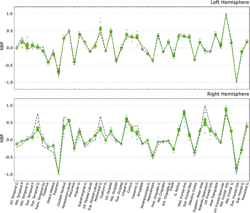
We quantified the global reliability of the NBPs as the correlation between DynCores obtained by the two analyses (r = 0.977, p < 0.001 and r = 0.936, p < 0.001 [for the right and the left hemisphere, respectively.]). We decided to use the mean DynCore of the combinatorial analysis as our reference DynCore (green lines, Figure 3) for the further analysis below.
3.3 Optimal scanning time estimation using whole-brain modeling
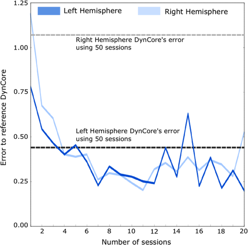
In order to determine a minimum scanning time large enough to produce a reliable DynCore, we performed a combinatorial analysis of 1 to 20 randomly-combined scans and assessed the Euclidean distance between the median DynCore at each step of the combinatorial analysis and the reference DynCore. Figure 4 shows this distance of the estimated DynCores as a function of the set size (or scan duration). For both hemispheres, we found that the error substantially decreases as more sessions were added. Note that already after adding four recordings this error reached asymptotic levels comparable to the distance between the reference DynCore and the DynCore estimated by concatenating all the 50 recordings from the same subject (gray dotted lines in Figure 3).
3.4 Dynamical core's single estimation consistency
As stated before, the clinical environment does not allow to have multiple estimations of the DynCore for each patient and then to use the median (as done in previous analyses). For this reason, we studied the Euclidean distance to the reference DynCore using each single DynCore estimation from the combinatorial analysis, that is, without computing each region's median as described above. We calculated the distance of each of these DynCores to the reference DynCore. To study to what extent a single estimation can capture subject's specific and also group-wise functional features of the brain, we performed the same combinatorial analysis using 50 rs-fMRI sessions from different participants (between-subjects analysis). Similar to what is shown in Figures 4 and 5 reveals that the Euclidean distance to the reference DynCore decreased as more data was added to the analysis both for the within-subject analysis and also for the between-subjects analysis. Note that although the distance never reached levels lower than those estimated using medians (Figure 4), it became relatively low after four recordings. This is especially true considering that in the within-subject analysis using all 50 recordings (dotted gray lines in Figure 3), the distance was ~0.5 for the left hemisphere and ~1.0 for the right hemisphere (thresholds values in Figure 4), which suggests that using 20 min of data from a single subject, is enough to study local brain dynamics of a single subject in a consistent way (as also suggested by Laumann et al., 2015).
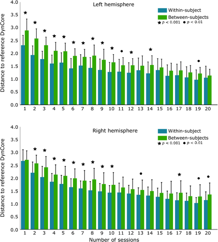
Interestingly, in the left hemisphere the difference between within and between distances required more recordings to lose statistical significance compared to that uncovered in the right hemisphere, which might indicate that the dynamics found in the left hemisphere are more individualized. Another observation supporting the notion of asymmetric functional specialization is represented in Figures 4 and 5, where the error in the left hemisphere using small number of sessions is smaller than error in the right hemisphere.
3.5 Region-wise variability using the whole brain model
To analyze how reliability is distributed in each brain region, we studied the mean local error, that is, the NBP absolute difference between each DynCore estimation and the reference DynCore, through the combinatorial analysis. We found that as more recordings were added, the estimation of the NBP in each region became more reliable (this is shown in Supporting Information Figure S1).
Then, we compared the overall between-subject and within-subject absolute mean local errors (shown in Supporting Information Figure S2), finding those regions where the within-subject mean local error was lower than that found in the between-subjects analysis. Furthermore, we explored the degree of consistency and reliability of each node by means of its relative nodal error difference (see Methods). Using this difference, we then ranked them in descending order, from high to low consistency (Figure 6a). After setting a minimum consistency threshold of 0.25, we found that 10 regions were simultaneously consistent in both hemispheres (Figure 6a), specifically the orbitofrontal cortex (superior frontal gyrus), olfactory cortex, anterior cingulate gyrus, amygdala, inferior parietal lobe, precuneus, paracentral lobe, thalamus, pallidum, and inferior temporal gyrus. The hippocampus showed an asymmetric behavior, as the left portion was between the most consistent nodes while the right portion presented a consistency near to zero (within-subject variability equal to between-subjects variability). Also, interesting is the fact that occipital regions seemed to have very low consistency values across both hemispheres, indicating a large inter-session variability.
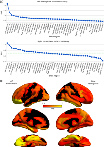
Finally, we studied the spatial distribution of the RNE (Figure 6b), finding a similar pattern in both hemispheres. Orbitofrontal and inferior temporal cortical parcels seemed to show increased RNE, while primary motor and sensitive cortices showed a similar pattern of decreased RNE.
4 DISCUSSION
In this study, we used whole-brain computational modeling (Deco & Kringelbach, 2016) to address the consistency of nodal and global metrics of multiple sessions of rs-fMRI from a single subject and single sessions from multiple subjects. We have shown that the DynCore reliably represents brain dynamics of a single subject in resting state, and that these parameters are consistent with group results. Additionally, we found that as the recording time gets larger, the DynCore estimation converges after concatenating four sessions of 5 min. We therefore propose that an optimal scan time for analysis of global and local brain dynamics on an individual level is in the order of 20 min. We have also shown that the proposed metrics not only capture the general properties of brain dynamics, but also that the DynCore can be used at a local scale, suggesting an optimal methodological scenario to study local and global brain dynamics consistently at a single-subject level, which is an important requirement to fully study neuropsychiatric disorders (Deco & Kringelbach, 2014).
This is not the first study trying to address reproducibility and consistency in resting state sessions. Many studies have shown that the longer the scanning time is, the better the consistency and reliability of the analysis is (Pannunzi et al., 2017). Interestingly, some have found that the optimal scanning time to have reproducible results is greater than 14 to 20 min (Anderson, Ferguson, Lopez-Larson, & Yurgelun-Todd, 2011; Birn et al., 2013; Laumann et al., 2015), which represents around three to four sessions in the present study, corroborating the idea of a minimal scanning time to have reproducible results. To extend this, another study (Kalcher et al., 2012) found that as the scanning time increases, the number of independent components found also increases monotonically also suggesting a better estimation of resting state dynamics by longer scanning times. Our results are in line with many findings addressing these issues (Anderson et al., 2011; Birn et al., 2013; Kalcher et al., 2012) and, in contrast to what now has become a common practice, 5 min (van Dijk et al., 2010) of scanning time may not be sufficient to produce reliable results on an individual level. A major limitation to the suggested 20-min scan length is the movement of the subject over such period, however, in this work we showed a good estimation of the DynCore can be obtained by using several shorter sessions (in this Case 4 sessions of 5 min).
Following this line of thinking, an interesting observation is that although we found symmetric profiles both for local standard deviation and error, symmetry for standard deviation was better explained by fewer recordings and weakened by adding more (Supporting Information Figure S1). This might suggest that although using multiple sessions is better to obtain a highly consistent estimation of the underlying functional organization of brain at rest, a plausible very slow physiological and/or environmental mediated variability (Taubert, Lohmann, Margulies, Villringer, & Ragert, 2011) of brain states could be overlooked using this approach. This might indicate that, to study very slow changes in the brain's functional organization, longitudinal rs-fMRI sessions must be processed in series of small batches. Like this, symmetry in variability patterns (error to grand-average DynCore and SDs) can reveal useful information to study changes in the brain at rest that occur over long periods of time (Taubert et al., 2011) that could ultimately be related to different, and not well studied physiological, cognitive, emotional, or even pharmacological factors.
At a whole-brain scale, the median value of the reference DynCore is 0.017, which indicates a critical oscillatory behavior optimally operating at the edge of a bifurcation (Deco & Jirsa, 2012; Deco, Kringelbach, et al., 2017). By exploring bifurcation parameter values from Figure 3 at a lobe scale, we were also able to identify that frontal lobe exhibited larger parameter dispersion (larger standard deviation) compared to occipital and temporal cortices, suggesting higher functional variability in the frontal lobe. Interestingly, a study (Anderson, Kinnison, & Pessoa, 2013) found that functional diversity in terms of cognitive domains varies across the brain. More importantly, frontal regions presented higher levels of diversity compared to other regions such as temporal and parietal cortices. A more specific and causal interpretation of local bifurcation values is beyond the scope of this study, but it is worth noticing that at least qualitatively, local NBPs display patterns that seem to relate with functional segregation. Also, supporting this idea is the fact that after performing a simple post-hoc analysis, nodes from the default mode network (as in van den Heuvel & Sporns 2011; van den Heuvel & Sporns, 2013) display a mean parameter value of 0.02, which is significantly closer to zero (p = 0.041) compared with the same mean value of 10,000 randomly bootstrapped subnetworks of the same size. Given that all these regions are considered hubs (van den Heuvel & Sporns, 2012; van den Heuvel & Sporns, 2013; Tomasi & Volkow, 2010), this suggests that local values closer to a transition or bifurcation state might also have central key role in information transfer. Future studies should explore with greater detail the functional role of local bifurcation dynamics in information trafficking and cognition.
Global consistency only makes sense in light of local consistency. This is an important consideration as regions presenting high within-subject consistency are not only better biomarker candidates, but might indicate important functional properties. For example, we found high consistency levels in the left and right orbitofrontal cortex (Figure 6). Interestingly, this region has been tightly linked with hedonistic experience (Kringelbach, 2005) and described as a sensory integration hub with multiple anatomical domains (Kringelbach & Rolls, 2004). The heterogeneity of both structure and function of this region might explain why at a single-subject level, its consistency is much larger than that extracted from multiple subjects as these characteristics might be highly individualized (Finn et al., 2015). Furthermore, the left superior orbitofrontal cortex was by far the most consistent of all regions, with a between-subject mean error four times larger than the within-subject mean error. This is interesting given that recently this region was described as one of the most important for maintaining brain dynamical organization (Deco, Van Hartevelt, et al., 2017).
Additionally, both precuneus and thalamus also showed high level of consistency in both hemispheres, suggesting that highly centralized cores (Deco, Van Hartevelt, et al., 2017; van den Heuvel & Sporns, 2011) might also be the ones reflecting higher consistency levels. This was corroborated after exploring the consistency (from Figure 6a) of the rich and binding club members (listed in Deco, Van Hartevelt, et al., 2017) where we found that 66% of the (8/12 nodes) rich club while 41% (5/12) of the binding club exhibited high consistency levels (Supporting Information Figure S3).
At the other side of the spectrum, within-subject consistency of visual and motor areas was as high or even lower as that found by using multiple subjects (Figure 6a and Supporting Information Figure S2), indicating that the variability of these regional dynamics is high and less individualized. Under a cognitive perspective, this makes sense as primary sensory information might be processed in similar ways across individuals. Finally, we found regions such as the hippocampus and the middle occipital gyrus that exhibited high consistency for one hemisphere but low in the other (Figure 6a) and that interestingly were in concordance with previous studies (Deco, Van Hartevelt, et al., 2017). These asymmetric profiles and other consistency considerations should be addressed carefully in future studies.
5 LIMITATIONS AND FUTURE CONSIDERATIONS
A primary limitation of the present study is the lack of single-subject structural connectivity matrices. Because current models (including the one presented here) of brain dynamics are based on the average structural information (Deco et al., 2014), it would be interesting to investigate if the number of sessions required to optimally reach the reference DynCore is smaller by using single-subject structural matrices. Finally, due to fMRI technical limitations, the temporal resolution is relatively low. Further modeling of resting state activity using MEG (Nakagawa et al., 2014) at a single subject level should also give richer insights into the behavior of local dynamics both in health and disease.
The parcellation used in this study (AAL) also represents a limitation because of the relative small number of regions in which the brain is parcellated and also the relative inhomogeneity inside each node, nevertheless as only young control subjects where used in this study, this should not be a mayor limitation (Gordon et al., 2014). However, in future works more advanced parcellation schemes should be used, combining surface based morphometry and multi-scale parcellation to analyze whole brain modeling based metrics in health and disease (Cammoun et al., 2012).
Additionally, as within-subject data was acquired in different days in a period of 6 months, the estimation of consistency could lead to an overestimation of the optimal minimum single-session scanning time as day-to-day variability might play an important role. In a clinical environment though, it seems more feasible to acquire 15–20 min in a single session than to split it up in different scanning sessions. Moreover, this split across different days also means that the day-to-day variability might not only produce an overestimation, but also produce valuable information about changes in brain organization only captured over longer periods. Future works should then analyze the consistency between long-length single session DynCores and multiple sessions DynCores.
Single subject dynamics as well as the shown variability of the estimated local consistency might operate differently across subjects. Because the aim of the current study was to address the consistency of brain dynamics using multiple sessions in one subject, it would be valuable to assess the same long-term consistency in other subjects using multiple sessions. This is especially true in light of recent findings showing accurate identification of subjects using functional fingerprints (Finn et al., 2015).
Dynamical properties of the brain, such as the neuronal variability (SD) (by means of the variability of the amplitude in the BOLD signal) (Martino et al., 2016) have shown to be plausible biomarkers for neuropsychiatric diseases, such as depression, mania, and bipolar disease (Magioncalda et al., 2015; Northoff et al., 2017). Additionally, other studies have shown that brain dynamics-based metrics, such as leading eigenvector dynamics analysis (LEiDA) associated with the cognitive performance in healthy older adults (Cabral et al., 2017). Therefore, in future steps the DynCore should be analyzed and compared with other dynamics-based features to describe pathological changes in the brain.
6 CONCLUSIONS
We presented a conceptual framework for analyzing local brain dynamics consistently at a single subject level by modeling resting state activity with a supercritical Hopf bifurcation model. The estimated intrinsic parameter, the DynCore, allowed us to explore the amount of information required to minimize the error in order to estimate consistent brain dynamics. Overall, including four sessions from the same subject yielded highly consistent results. Importantly, we showed a heterogeneous consistency variability across the brain. Already known brain hubs showed higher consistency within the same subject while the consistency found in primary visual and motor areas was only as high as that found using recordings from multiple subjects. This heterogeneity is a reflection of highly individualized dynamics that point toward useful clinical applications. These methods open new avenues to analyze local brain dynamics at a single subject level that may reveal individualized aspects of the healthy and diseased brain.
ACKNOWLEDGMENTS
In this work, Patricio Donnelly-Kehoe was supported by a PhD grant from the National Scientific and Technical Research Council—Argentina (CONICET). Victor M Saenger was supported by the Research Personnel Training program (PSI2013-42091-P) funded by the Spanish Ministry of Economy and Competitiveness. Morten Kringelbach is supported by the ERC Consolidator Grant CAREGIVING (no. 615539) and the Center for Music in the Brain, funded by the Danish National Research Foundation (DNRF117). Gustavo Deco was supported by the European Research Council (ERC) Advanced Grant DYSTRUCTURE (no. 295129). Simone Kühn has been funded by two grants from the German Science Foundation (DFG KU 3322/1-1, SFB 936/C7), the European Union (ERC-2016-StG-Self-Control-677804) and a Fellowship from the Jacobs Foundation (JRF 2016-2018).
CONFLICT OF INTEREST
None to declare.


