A MATLAB toolbox for multivariate analysis of brain networks
Funding information: National Institute of Biomedical Imaging and Bioengineering, Grant/Award Numbers: K25 EB012236, ES008739, R01; National Institute of Environmental Health Sciences, Grant/Award Number: R01 ES008739; Wake Forest Clinical and Translational Science Institute, Grant/Award Number: UL1 TR001420
Abstract
Complex brain networks formed via structural and functional interactions among brain regions are believed to underlie information processing and cognitive function. A growing number of studies indicate that altered brain network topology is associated with physiological, behavioral, and cognitive abnormalities. Graph theory is showing promise as a method for evaluating and explaining brain networks. However, multivariate frameworks that provide statistical inferences about how such networks relate to covariates of interest, such as disease phenotypes, in different study populations are yet to be developed. We have developed a freely available MATLAB toolbox with a graphical user interface that bridges this important gap between brain network analyses and statistical inference. The modeling framework implemented in this toolbox utilizes a mixed-effects multivariate regression framework that allows assessing brain network differences between study populations as well as assessing the effects of covariates of interest such as age, disease phenotype, and risk factors on the density and strength of brain connections in global (i.e., whole-brain) and local (i.e., subnetworks) brain networks. Confounding variables, such as sex, are controlled for through the implemented framework. A variety of neuroimaging data such as fMRI, EEG, and DTI can be analyzed with this toolbox, which makes it useful for a wide range of studies examining the structure and function of brain networks. The toolbox uses SAS, R, or Python (depending on software availability) to perform the statistical modeling. We also provide a clustering-based data reduction method that helps with model convergence and substantially reduces modeling time for large data sets.
1 INTRODUCTION
Complex brain network analysis has gained increasing interest over the past decade or so. Network models of the brain have provided valuable insight into the structure and function of the brain as an integrated system with complex neural interactions (Sporns, 2014). Complex physiological, cognitive, and behavioral responses result from interactions among vast numbers of neurons within local circuits as well as interactions between such circuits (Sporns, 2010). Thus, network analysis of the brain provides a profound perspective into understanding the structural and functional organizations of the brain in health and disease (Bassett & Bullmore, 2009; Bullmore & Sporns, 2009; Sporns, 2010). Increasing numbers of studies indicate alterations in network configuration of the brain with aging (Meunier, Achard, Morcom, & Bullmore, 2009; Micheloyannis et al., 2009; Sala-Llonch, Bartres-Faz, & Junque, 2015), and in neurological disorders such as Alzheimer's disease (Fang et al., 2015; He, Chen, & Evans, 2008; Stam et al., 2009; Supekar, Menon, Rubin, Musen, & Greicius, 2008), schizophrenia (Bassett et al., 2008; Liu et al., 2008; Rubinov et al., 2009), depression (Leistedt et al., 2009; Spielberg et al., 2016; Ye et al., 2015), and Parkinson's disease (Gao & Wu, 2016; Tessitore et al., 2017).
Structural and functional brain networks can be generated using modern non-invasive neuroimaging techniques such as diffusion MRI (magnetic resonance imaging), functional MRI, EEG (electroencephalography), MEG (magnetoencephalography), and functional NIRS (near-infrared spectroscopy). Brain networks constructed from such neuroimaging data are usually analyzed using graph theoretical methods. Graph vertices represent brain regions, and (weighted/binary) edges between vertices represent the structural or functional connections (quantified by correlation or other methods). Graph theoretical methods have allowed evaluating complex networks by quantifying such networks through meaningful and easily computable features, such as local and global efficiency (Rubinov & Sporns, 2010).
Despite the exponential increase in brain network studies and promising results, development of multivariate frameworks for relating networks to phenotypic characteristics and drawing inference from such relationships, especially for whole-brain networks, has lagged behind (Simpson, Bowman, & Laurienti, 2013; Simpson & Laurienti, 2016). Simpson and Laurienti (2015) developed a multivariate mixed effects modeling framework in response to such needs. This framework allows comparing whole-brain functional connectivity patterns between groups, quantifying the relationship between covariates and connectivity patterns while reducing spurious correlations, predicting phenotype from network structure, and simulating brain networks. The flexibility of the model also allows controlling for confounding covariates such as sex. Any neuroimaging data capable of representing structural or functional brain networks can be used within this framework to study the effects of global and local brain network topology on physiological, behavioral, and cognitive processes.
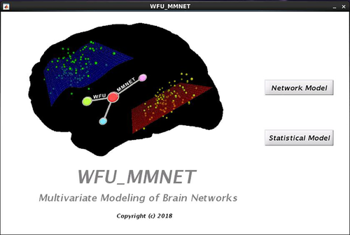
In the present manuscript we present a MATLAB toolbox, with a graphical user interface (GUI), for the application of this modeling framework (Figure 1—The brain network shown in this figure was generated [for illustrative purposes only] using BrainNet Viewer toolbox [Xia, Wang, & He, 2013]). The toolbox, called WFU_MMNET (Multivariate Modeling of Brain Networks), is designed to make this framework more accessible to neuroscientists working on neuroimaging data, as well as more experienced statisticians who use neuroimaging data for brain network analysis. WFU_MMNET is implemented in MATLAB and calls SAS, R, or Python (depending on software availability) to perform the statistical modeling. Data sets utilized within this framework are usually big, containing thousands of brain connections for each participant. MATLAB is currently not capable of, or very slow in, modeling such big correlated data sets. However, implemented packages and modules in SAS, R, and Python allow modeling such data sets in a much faster and more flexible way. We also provide a clustering-based data reduction method that helps with model convergence and substantially reduces modeling time for large data sets (especially when using R).

2 MATERIALS AND METHODS
2.1 Software and data sharing
The toolbox, manual, and a sample case study, including the data and results, are provided on NITRC - https://www.nitrc.org/projects/wfu_mmnet.
2.2 Overview of the use of the toolbox
WFU_MMNET was developed in MATLAB (R2016b) under a 64-bit Linux platform. MATLAB versions above R2014b should be fine to use. The user needs to have MATLAB and one of SAS, R, or Python (preferably SAS or R as they use a random-effects approach in estimating the parameters and can accommodate multiple random effects which make them more appropriate for our framework) installed on Linux prior to using the toolbox. However, if the modeling software (SAS, R, or Python) is installed in Windows, the user can still perform the modeling by using the generated modeling files in Windows (full detail is provided in the user manual). The method implemented in WFU_MMNET is a regression framework. Since brain connectivity patterns are correlated within each study participant (i.e., repeated measurements are used), a mixed-effects regression framework is used to capture, and account for, the correlation between measurements of each participant. The focus of the toolbox is to perform statistical comparisons of brain networks (local or global) between study populations and to identify associations between brain network topology and covariates of interest. WFU_MMNET was specifically developed as a statistical analysis toolbox that accepts preprocessed data as an input. Specifics of the format and type of input data are described below and in the user manual. The toolbox does not perform raw data preprocessing as different types of neuroimaging data and different investigators have separate approaches toward preprocessing the raw data.
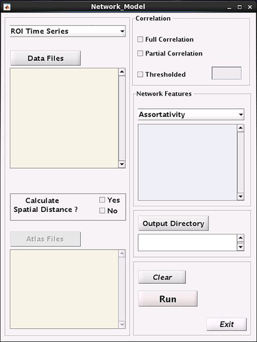
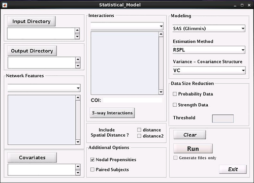
The graphical user interface (GUI) allows users without extensive MATLAB, SAS, R, or Python programming experience to perform statistical group comparisons and assess statistical associations between network topology and covariates of interest. The starting GUI is shown in Figure 2. Modeling is done in two main steps. We have deliberately divided it into two steps for an easier, flexible, and more efficient analysis. In the first step, using imaging data files, initial modeling files, such as an initial data frame, are constructed. Then, using these files, final modeling files, including equations, options, and data sets are generated, and statistical models are fitted. The first step is independent of the second step, and can be repeated for making different data frames of different imaging data or making different data frames for different options on the same imaging data. This step is done through the “Network_Model” GUI (Figure 3). The second step can also be done independently as long as data frames are available. This step is done using the “Statistical_Model” GUI (Figure 4).
2.3 Supported data formats
Structural networks represent maps of white matter tracks between all pairs of brain regions, and are usually constructed from diffusion MRI such as diffusion tensor imaging (DTI) and diffusion weighted imaging (DWI) data. To model the structural networks, connection matrices quantifying the connectivity between brain regions should be used as the input data.
To model the functional networks, either time series data or connection matrices should be first computed from the preprocessed data. If time series are used, the toolbox automatically computes the connection matrices. The toolbox includes full and partial correlation (the user can select either one) for computing the connection matrices as they are the most commonly used association measures. However, other methods such as coherence and mutual information have also been used in some network studies. If the user wishes to use methods other than full or partial correlation, the connection matrices should be computed prior to using WFU_MMNET and loaded into the toolbox instead of time series. FMRI users can also load (preprocessed) 4d voxel-wise time series (i.e., a time series of preprocessed functional images) and an atlas defining ROIs. WFU_MMNET extracts ROI time series from 4d files and the loaded atlas, and computes the correlation between the ROIs.
The toolbox thresholds the connection matrices by default to remove the negative correlations as multiple graph features, clustering in particular, remain poorly understood in networks with negative connections (Fraiman, Balenzuela, Foss, & Chialvo, 2009; Telesford, Simpson, Burdette, Hayasaka, & Laurienti, 2011). In the current version of the toolbox, there is no option to retain the negative associations. This is an active area of research that may be included in future versions of the toolbox. A density thresholding option is provided to remove weak connections. However, this is not a default option as weak connections might represent local bridges in the network, and also for the reasons discussed in (Honey et al., 2009).
2.4 Topological network features
This toolbox uses the Brain Connectivity Toolbox (BCT) (Rubinov & Sporns, 2010) to compute the topological network features. Thus, BCT should be added to the MATLAB search path before using WFU_MMNET. The most common features of network segregation (clustering coefficient, transitivity [Onnela, Saramaki, Kertesz, & Kaski, 2005], modularity, local efficiency), integration (path length, global efficiency), centrality (degree, betweenness centrality, eigen-vector centrality, leverage centrality [Joyce, Laurienti, Burdette, & Hayasaka, 2010]), and resilience (assortativity coefficient, density) have been made available in this toolbox. The BCT has several other network features that were not included in this toolbox at this time. For the path length, global efficiency, and transitivity, unlike BCT that returns a single (averaged) value, the toolbox uses the nodal values. The nodal values for these three features will be computed using the equations referenced in (Rubinov & Sporns, 2010).
2.5 Modeling framework
WFU_MMNET models the connectivity patterns using a two-part mixed-effects modeling framework developed by Simpson and Laurienti (2015). The relationship between both the probability (presence/absence) and strength of a connection, as the outcome (dependent) variables, and different sets of covariates including dyadic or overall network features, covariates of interest and demographics, as independent variables, is quantified through this framework. It also allows assessing how the effects of covariates of interest on the brain connections and brain networks vary in different study populations. The flexibility of the model also allows reducing spurious correlations by controlling for important confounding variables such as spatial distance between brain regions and sex. The two-part mixed-modeling approach is briefly described below. More detail can be found in the referenced paper.
 (1)
(1) (2)
(2) (3)
(3) (4)
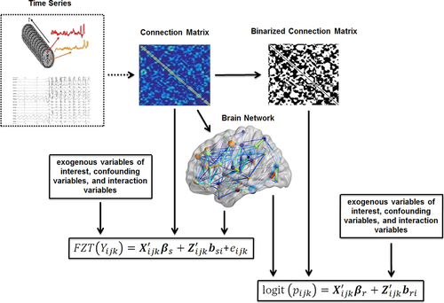
(4)Where X ijk is the design matrix for the fixed effects (β r and β s), Z ijk is the design matrix for the random effects that is analogous to X ijk for the fixed effects, and ε ijk captures the random noise in the connection strength between node j and node k for the ith participant. Equation 3 is a logistic regression equation quantifying the relationship between the connection probability and covariates. Equation 4 quantifies the relationship between the strength of present connections and the same set of covariates. FZT is the Fisher's Z-transform applied to ensure the normality assumption is met. The modeling results contain the estimates (β r and β s values) and significance of estimates (p-values) in both models. Figure 5 shows the diagram of the modeling approach (partially recreated from [Bahrami et al., 2017]). We have provided a sample case study in Supporting Information Appendix and on NITRC in which different steps of the modeling process are briefly described in combination with a sample data set. We have also provided the data and results from each step to allow the users repeat each step and compare the results.
2.6 Modeling software
WFU_MMNET calls either one of SAS, R, or Python in the modeling part. SAS and R use generalized linear mixed models (GLMMs) to model the probability (Equation 3) and strength (Equation 4) of brain connections. GLMMs allow modeling correlated data sets where the response is not necessarily normally distributed (as is the case when modeling connection probability). Python uses the generalized estimating equations (GEE) approach that precludes the use of the random effects in Equations 3 and 4, but still accounts for within-participant correlations. Unfortunately, a GLMMs-based module is not available at this time in Python. In future versions, the implemented GEE approach will be replaced by a GLMMs-based module as soon as such module is introduced for Python.
Modeling of both probability and strength of brain connections is done through the GLIMMIX procedure in SAS. GLIMMIX can model data sets with any distribution in the exponential family (e.g., binary, binomial, and Poisson) conditional on the assumption that random effects are normally distributed. GLIMMIX can estimate the parameters through several pseudo-likelihood techniques or a maximum likelihood (ML), restricted ML, or quasi-likelihood approach. Multiple options are provided in GLIMMIX which make it very efficient, fast, and flexible in modeling big correlated data sets. However, to maintain user-friendliness, we have just included options for choosing the estimation method and variance–covariance structure given that they are the most important options.
For analyses that utilize R, modeling of both probability and strength of brain connections is conducted through functions implemented in lme4 package (Bates, Machler, Bolker, & Walker, 2015). lme4 provides functions for fitting linear (lmer), generalized linear (glmer), and nonlinear (nlmer) mixed models. This toolbox uses lmer and glmer to model the strength and probability of brain connections, respectively. However, since lme4 does not conduct statistical tests on lmer objects (i.e., p-values are not computed) we use the lmerTest package (Kuznetsova, Brockhoff, & Christensen, 2015) which employs functions implemented in lme4 but also conducts tests on lmer objects providing p-values for both the probability and strength models. Thus, the lmerTest package should be installed if R is chosen as the modeling software. This package, like GLIMMIX in SAS, uses pseudo-likelihood or maximum likelihood techniques in estimating the parameters. However, it has limited options, and is slower when compared to GLIMMIX. GLIMMIX and lme4 produce the same parameter estimates and p-values (assuming the same estimation method is chosen for both) as shown in Section 3.2.
While using the same modeling framework as in SAS and R, parameters in Python are estimated via a generalized estimating equation (GEE) approach for two reasons: (a) GLMMs frameworks are not yet available in Python, preventing modeling of the brain connection probability. (b) For larger data sets (larger numbers of participants and ROIs) GEE estimates are close to the GLMMs estimates while being less computationally expensive. Unlike GLIMMIX and lme4 which use likelihood estimation techniques and allow incorporation of participant- and nodal-specific random effects, the GEE approach employs a population average model that uses a generalized estimating equation to estimate model parameters. GEE is especially useful when likelihood-based approaches in SAS—GLIMMIX or R—lme4 do not converge or increase the modeling time in a significant way. This could happen when modeling very big data sets with a large number of participants and/or ROIs (this is demonstrated in a sample data set below). Also, GEE provides unbiased estimates when variance–covariance structure is improperly defined. However, since Python - GEE cannot accommodate for multiple sources of random effects like SAS—Glimmix and R—lme4, parameter estimates obtained from GEE could be different than those obtained from SAS or R, especially when modeling data sets with small numbers of participants or ROIs. The difference between the results obtained from GEE with those from GLIMMIX and lme4 gets much smaller when modeling larger data sets (this is demonstrated below). Further detail about advantages and disadvantages of both approaches (GEE and GLMMs) is provided in the discussion.
2.7 Data size reduction
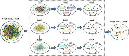
Brain network data sets typically contain thousands of brain connections for each participant, even for a small number of ROIs. This sometimes results in a lack of convergence or increases the modeling time significantly for the mixed modeling approach, particularly when modeling the probability of brain connections (logistic regression in Equation 3) with nodal random effects (nodal propensities) included. To address this issue, we have provided a clustering-based data size reduction method. For this method, data samples of each participant are treated as a big cluster and further split into sub-clusters through a k-means clustering method. Then, data samples closest to the center of each cluster are retained and other samples are discarded. The number of clusters is determined through the selected threshold (percentage of the data that is selected to be removed). This approach allows preserving the same number of data samples for each participant. Figure 6 illustrates how three samples are selected from each participant's data through the implemented data size reduction method. The performance of this method was evaluated using a sample data set (see Section 3.3).
3 RESULTS
3.1 WFU_MMNET results
WFU_MMNET provides two tables presenting the estimation coefficients and p-values of modeling the probability and strength of brain connections. Tables are similar to the ones shown in Table 1. Additional columns including SE, degrees of freedom (DF), and t values provided in the actual tables are not shown here.
| Probability model | Strength model | ||||
|---|---|---|---|---|---|
| Effect | Estimate | *p-value | Effect | Estimate | *p-value |
| Intercept | βr0 | Pvalr0 | Intercept | βs0 | Pvals0 |
| NetF1 | βrNetF1 | PvalrNetF1 | NetF1 | βsNetF1 | PvalsNetF1 |
| NetFN1 | βrNetFN1 | PvalrNetFN1 | NetFN1 | βsNetFN1 | PvalsNetFN1 |
| COI | βrCOI | PvalrCOI | COI | βsCOI | PvalsCOI |
| Ex_Cov1 | βrEx_Cov1 | PvalrEx_Cov1 | Ex_Cov1 | βsEx_Cov1 | PvalsEx_Cov1 |
| Ex_CovN2 | βrEx_CovN2 | PvalrEx_CovN2 | Ex_CovN2 | βsEx_CovN2 | PvalsEx_CovN2 |
| NetF1 × COI | βrNetF1 × COI | PvalrNetF1 × COI | NetF1 × COI | βsNetF1 × COI | PvalsNetF1 × COI |
| NetFN1 × COI | βrNetFN1 × COI | PvalrNetFN1 × COI | NetFN1 × COI | βsNetFN1 × COI | PvalsNetFN1 × COI |
- N1: number of selected network features.
- N2: number of exogenous covariates.
This table shows how covariates of interest relate to the probability (i.e., presence/absence or density) and strength (i.e., correlation coefficient or other measure of association) of brain connections. More specifically, each parameter presented in Table 1—Probability Model (i.e., βrNetF1, …, βrNetFN1 × COI), represents the change in the log odds of an edge existing (therefore the probability of an edge existing) for each unit change in the given covariate. Each parameter presented in Table 1—Strength Model (i.e., βsNetF1,…, βsNetFN1 × COI), represents the change in the average strength of a connection for each unit change in the given covariate. In a typical analysis, the study populations will be coded in the covariate of interest (COI). The direction and significance of each covariate in explaining the connectivity patterns (presence/absence and strength) are exhibited in these tables. For example, in a study with two populations, estimates and p-values for the network features (βrNetF1,…, βrNetFN1, PvalrNetF1,…, PvalrNetFN1 and βsNetF1,…, βsNetFN1, PvalsNetF1,…, PvalsNetFN1) represent how the selected network features (e.g., clustering coefficient, modularity) affect the probability and strength of brain connections in the baseline group, and estimates for the interaction covariates (βrNetF1 × COI,…, βrNetFN1 × COI, PvalrNetF1 × COI,…, PvalrNetFN1 × COI, and βsNetF1 × COI,…, βsNetFN1 × COI, PvalsNetF1 × COI,…, PvalsNetFN1 × COI) represent the additional effects of the selected networks features in the second population. If more than two populations are studied, the estimates for the interaction covariates represent the additional effects of each population when compared to the baseline population.
Estimates and p-values for the exogenous covariates (βrEx_Cov1,…, βrEx_CovN2, PvalrEx_Cov1,…, PvalrEx_CovN2, and βsEx_Cov1,…, βsEx_CovN2, PvalsEx_Cov1,…, PvalsEx_CovN2) represent how the selected exogenous covariates such as age, or disease risk factors (e.g., hypertension or smoking) affect the probability and strength of brain connections. Adding an interaction of each exogenous covariate with the COI shows if the effect of the given covariate on the probability and strength of brain connections is different between study populations (this is not shown here). In summary, each parameter estimate represents the effect of a given covariate on the probability or strength of brain connections, and its interaction estimate represents the additional effect in the other study populations (groups).
3.2 SAS, R, and Python overlap
We assessed the overlap among the results obtained from SAS (Glimmix), R (lmerTest), and Python (Statsmodels-GEE) using two data sets with different numbers of participants and ROIs. The first study (Simpson & Laurienti, 2015) examined differences in brain networks between younger and older adults. For the second study, we used preprocessed resting-state fMRI data of 80 participants from the Human Connectome Project (HCP) (Van Essen et al., 2013). We used this data only to assess how the overlap between the modeling software packages changes for larger numbers of participants and ROIs. For the second study, we randomly split the participants into two groups of 42 and 38, using group membership as our covariate of interest. For each data set, the same fixed-effects, random-effects (except for Python – GEE which cannot accommodate multiple random effects), and the same modeling options were used. Comparisons were made through computing the correlation and normalized squared Euclidean distance (Wolfram, 2010) between estimation coefficients and p-values obtained from the three methodologies. We used SAS v.9.4, R v.3.3, and Python v.2.7 in our analyses. (The user only needs one of these modeling software packages installed. Also, other versions can be used as long as the required packages are installed.)
We used more than one random effect in SAS and R models when assessing the overlap as the modeling framework presented in Simpson and Laurienti (2015), and implemented in this software, uses more than just a random intercept. Dyadic network features could also be sources of correlation between samples (i.e., dyadic network features at different connections of a participant's brain network are not independent from each other). Moreover, nodal propensities to establish connections to other nodes (above and beyond what is accounted for by dyadic properties) are other important sources of correlation (random effects) that should be accounted for.
3.2.1 Aging study
Aging data used here were resting-state fMRI scans from 39 participants (healthy young adults: 20, healthy older adults: 19) that has previously been used (Hugenschmidt, Mozolic, Tan, Kraft, & Laurienti, 2009; Simpson & Laurienti, 2015). A brain network from each participant was constructed using time series of 90 ROIs using Automated Anatomic Labeling atlas (Tzourio-Mazoyer et al., 2002). The same fixed effects were used for all three analyses: (a) Covariate of interest (COI): age group as a binary variable; (b) network features: the average of the following network features in each nodal pair: clustering coefficient, global efficiency, degree (difference instead of average), and overall modularity; (c) Confounding variables: age, education, sex, spatial distance, and square of spatial distance; and (d) interactions of the network features and sex with COI. The same random effects accounting for network features (clustering coefficient, global efficiency, and degree difference), as well as spatial distance and square of spatial distance were used in SAS and R models. A single random intercept was used in the Python model as it cannot accommodate multiple random effects. The overlap between the results is shown in Table 2.
| Software | Coeff (Corr) | Coeff (Dist) | Pval (Corr) | Pval (Dist) |
|---|---|---|---|---|
| SAS and R (probability) | 1.0000 | 2.3990e-07 | 0.9798 | 0.0103 |
| SAS and R (strength) | 1.0000 | 1.5389e-10 | 1.0000 | 1.0142e-05 |
| SAS and Python (probability) | 0.5359 | 0.2816 | 0.4124 | 0.2970 |
| SAS and Python (strength) | 0.4248 | 0.2897 | 0.6702 | 0.1650 |
| R and Python (probability) | 0.5363 | 0.2813 | 0.4245 | 0.2901 |
| R and Python (strength) | 0.4247 | 0.2897 | 0.6727 | 0.1638 |
As Table 2 presents, the estimates and p-values obtained from Python are very different than those obtained from SAS and R. This is due to the different approach that is used in Python - GEE compared to the ones used in SAS – Glimmix and R-lme4 in estimating the parameters. However, for the reasons discussed in Hubbard et al. (2010), GEE estimates become more accurate the larger the data sets being modeled become. Thus, GEE may be used in modeling large data sets and when the other two software programs are not available. To see how modeling larger data sets (i.e., larger numbers of ROIs and participants) affects the overlap between Python estimates and those of SAS and R, we modeled another data set that includes more participants and more ROIs for each participant's brain network.
3.2.2 HCP study
Data used here were preprocessed resting-state fMRI data from 80 HCP participants. We used this data only to assess how the overlap between the modeling software packages changes for larger numbers of participants and ROIs, thus details of the data have been omitted. A brain network was constructed for each participant using time series from 116 ROIs (using AAL atlas including the cerebellum). The same fixed effects listed below were used in all three analyses: (a) covariate of interest (COI): a binary variable distinguishing the 80 participants into two random populations (groups of 38 and 42); (b) network features: the average of the following network features in each nodal pair: clustering coefficient, global efficiency, degree (difference instead of average), and overall modularity; (c) seven randomly generated covariates including five continuous variables, one binary variable, and a categorical variable with three levels; (d) interactions of the network features with COI; (e) spatial distance, and square of spatial distance between brain regions. We used random effects accounting for network features (clustering coefficient, global efficiency, and degree difference), as well as spatial distance and square of spatial distance. As Table 3 shows, the overlap between results obtained from Python and those of SAS and R has noticeably improved despite using the same random effects as the ones in Section 3.2.1. The higher overlap is probably due to the larger number of participants (and ROIs) as well as larger number of exogenous variables when compared to the aging data. This shows the promise of using Python – GEE in modeling large data sets when the user does not have access to SAS or R, or in cases where modeling in SAS and R results in convergence issues or increases the modeling time dramatically.
| Software | Coeff (Corr) | Coeff (Dist) | Pval (Corr) | Pval (Dist) |
|---|---|---|---|---|
| SAS and R (probability) | 1.0000 | 8.6127e-06 | 0.9992 | 4.3207e-04 |
| SAS and R (strength) | 1.0000 | 1.8490e-10 | 1.0000 | 4.6673e-04 |
| SAS and Python (probability) | 0.9644 | 0.0191 | 0.7207 | 0.1405 |
| SAS and Python (strength) | 0.9831 | 0.0091 | 0.6677 | 0.1663 |
| R and Python (probability) | 0.9648 | 0.0187 | 0.6976 | 0.1519 |
| R and Python (strength) | 0.9831 | 0.0091 | 0.6696 | 0.1653 |
3.3 Modeling time
The statistical modeling (parameter estimation) time depends on the utilized system (e.g., CPU speed and Cache size), number of subjects and ROIs as well as the utilized statistical modeling software (i.e., SAS, R, or Python) for parameter estimation. Table 4 shows the statistical modeling time for three resting-state fMRI data sets with different number of subjects and ROIs in SAS, R, and Python on a 64-bit Linux platform (CPU: 1400 MHZ, Cache size: 2048 KB). Also, the number of fixed effects, random effects, categorical variables and the version of the statistical modeling software might affect the modeling time. We used 16, 19, and 18 fixed effects and 6, 6, and 7 random effects in the three models with 30, 80, and 200 participants (Table 4), respectively. The total running time is mostly determined by the statistical modeling (parameter estimation) time, especially for large data sets. However, choosing partial correlation for computing the connectivity matrices (when starting with time series), using a separate atlas for each subject in computing the distance matrices, using older MATLAB versions, and larger numbers of subjects, ROIs, and fixed and random effects can increase the total (network and statistical) running time. Modeling was done using MATLAB (R2016b), SAS v.9.4, R v.3.3, and Python v.2.7. As the table presents, modeling time could be a problem when large data sets are modeled in R. The slower modeling time in R could be attributed to its single threaded nature when compared to SAS and Python.
| Subjects | ROIs | SAS | R | Python | |
|---|---|---|---|---|---|
| Probability model | 30 | 90 | 6.80 | 1,529.60 | 3.27 |
| Strength model | 30 | 90 | 3.21 | 152.8 | 3.06 |
| Probability model | 80 | 116 | 39.02 | 14,903.87 | 16.98 |
| Strength model | 80 | 116 | 32.13 | 1941.71 | 19.80 |
| Probability model | 200 | 268 | 536.88 | 244,457.35 | 329.66 |
| Strength model | 200 | 268 | 114.10 | 47,681.40 | 136.80 |
3.4 Data size reduction
As discussed in Section 2.7, another methodological approach in WFU_MMNET intended to deal with convergence issues or excessive modeling time is a data size reduction option. Adding nodal propensities to the random effects of the HCP data set used in Section 3.2.2 resulted in a lack of convergence in the probability model. However, using the implemented data size reduction method, when this data set was reduced to 90% of its original size, the convergence problem was resolved (SAS was used as the modeling software here).
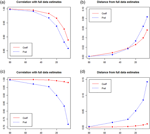
To further evaluate the performance of the implemented data size reduction method, the parameter estimates obtained from modeling the full HCP data set (without nodal propensities) and those obtained from the reduced data were compared (using the same fixed, random effects, and modeling options as in Section 3.2.2). Again, correlation and distance of estimates and p-values obtained from modeling the full data set with those obtained from modeling reduced versions of this data set (at six different thresholds: retain 80%, 50%, 30%, 20%, 10%, 5%) were computed (SAS was used in all modeling runs). As Table 5 shows, parameter estimates obtained from modeling the reduced versions of the HCP data are almost the same as those obtained from modeling the full data set even when a high percentage of the data is removed. Results are also shown in Figure 7 for illustrative purposes.
| Probability model | Strength model | |||||||
|---|---|---|---|---|---|---|---|---|
| Data size (%) | Coeff (Corr) | Coeff (Dist) | Pval (Corr) | Pval (Dist) | Coeff (Corr) | Coeff (Dist) | Pval (Corr) | Pval (Dist) |
| 80 | 0.9996 | 0.0011 | 0.9981 | 0.0010 | 0.9998 | 0.0001 | 0.9965 | 0.0018 |
| 50 | 0.9956 | 0.0086 | 0.9911 | 0.0046 | 0.9986 | 0.0008 | 0.9705 | 0.0150 |
| 30 | 0.9835 | 0.0180 | 0.9677 | 0.0169 | 0.9963 | 0.0019 | 0.9543 | 0.0246 |
| 20 | 0.9664 | 0.0255 | 0.9382 | 0.0329 | 0.9920 | 0.0040 | 0.8988 | 0.0509 |
| 10 | 0.9274 | 0.0397 | 0.8808 | 0.0636 | 0.9856 | 0.0073 | 0.8311 | 0.0852 |
| 5 | 0.8885 | 0.0558 | 0.8584 | 0.0831 | 0.9796 | 0.0103 | 0.7168 | 0.1424 |
4 DISCUSSION
This manuscript details a MATLAB toolbox with a graphical user interface that was developed in response to the need to bridge an important gap between network analyses of the brain and multivariate statistical inferences associated with such analyses. The freely-available GUI presented with this toolbox allows those without programming experience in MATLAB, SAS, R, or Python to use the implemented multivariate framework to perform multiple analyses on brain network data, including: (a) assessing the effects of covariates of interest such as age, disease phenotypes, and risk factors on the density and strength of brain connections in global and local brain networks; (b) assessing if the effects of such covariates on the density or strength of brain connections is different between study populations (e.g., if the impact of hypertension on brain connections is different between older and younger people); (c) assessing the effects of topological network features such as clustering coefficient and modularity on the density and strength of brain connections in different study populations, which in turn allows evaluating possible brain network differences between such populations, and the contribution of covariates of interest to such differences. The flexibility of the implemented framework also allows controlling for important confounding variables such as sex and spatial distance between brain regions.
Although the implemented modeling framework was initially introduced for whole-brain network analyses in Simpson and Laurienti (2015), this toolbox can also be used to evaluate network properties of brain sub-networks. However, when assessing sub-networks, some accuracy in computing the topological network features such as global efficiency and degree may be lost due to excluding connections between the regions located within the selected sub-network and the remainder of the brain.
The toolbox can be used by a wide range of people studying the structural or functional organizations of brain networks, and the impacts of covariates on brain connections and brain networks, as it allows using a variety of neuroimaging data. This is important as different neuroimaging techniques measure different physiological processes and physical interactions in the brain, and at different temporal and spatial resolutions. Thus, this software provides principled and widely applicable tools that can provide neuroscientific insight at multiple scales.
Data sets generated and used in this toolbox are usually big as they consist of thousands of brain connections for each participant, even for a small number of brain regions. This prevents using the toolbox for voxel-wise brain network analysis, and might result in convergence or modeling time issues when a large number of ROIs and participants are used. Two separate approaches are accessible in this toolbox to address this limitation. The first one is to use the clustering-based data size reduction method. The second option is to use the Python-GEE as the modeling software. Although as shown in Section 3.2.2 the results obtained from GEE are close to those obtained from SAS-Glimmix and R-lme4 for larger data sets, there are key differences between the approach that Python - GEE employs in estimating the parameters and the ones that SAS-Glimmix and R-lme4 use that lead to large differences in results for smaller data sets. We strongly suggest using SAS or R because they allow incorporating multiple random effects and explaining individual variation in the impacts of predictors on the response variables (density or strength of brain connections in our case), and the literature also appears to favor the random-effect (GLMM) approach (Hubbard et al., 2010). However, for larger data sets when the user does not have access to SAS or R, or faces a lack of convergence or modeling time increases dramatically, Python might be a good alternative. The comparison between the GEE and random-effects approaches toward estimating the parameters is not within the scope of this article but, two main differences are: (a) GEE is a population averaged approach (i.e., the parameter estimate is the effect of change in the mean outcome for a predictor unit change across all participants), while the random-effects is a participant-specific approach (i.e., a random-effects parameter estimate is the effect of change in the mean outcome for predictor unit change of a particular individual or participant); (b) GEE cannot accommodate multiple sources of random effects as it models the correlation as a nuisance variable (i.e., as a covariate). However, GEE estimates are generally more robust against model misspecifications since random-effects require distributional assumptions and proper covariance structure specification. More detail can be found in (Fitzmaurice, Laird, & Ware, 2012; Gardiner, Luo, & Roman, 2009; Heagerty & Zeger, 2000; Hubbard et al., 2010). In future versions, we will be replacing the GEE-based approach with a GLMMs-based approach as soon as a Python module is introduced.
The toolbox in this study was developed in MATLAB; but, it calls either one of SAS, R, or Python to conduct the modeling part as MATLAB is currently not capable of or very slow in modeling large data sets produced within the implemented framework. Thus, the user needs to have SAS, R (with the required package: lmerTest), or Python (with the required modules: statsmodels, numpy, scipy, and pandas) installed on Linux. The default software is set to SAS as it employs the random-effect approach in estimating the parameters, and also is much faster and more flexible (e.g., it checks multiple convergence criteria and allows using several estimation methods and variance–covariance structures for the random effects). However, we have only provided options to choose the estimation method and variance–covariance structure for the purposes of simplicity and usability in the current version.
An important potential of the modeling framework implemented in this toolbox is its capability for multimodal network analysis. Multimodal analysis is not accessible through the current version of this toolbox. However, the needed methodological extensions are being developed and this capability will be added to future versions to allow combining two or more data sets acquired with different neuroimaging techniques. This will allow evaluating the association between brain physiological processes and its structure from a network perspective while benefiting from spatiotemporal resolution complementarity. For example, this allows evaluating how functional network properties of different brain regions and functional connections between them are associated with the structural network features and structural connection between them as well as evaluating the impact of different covariates on such networks and connections. Future versions will also provide more modeling options and visualization interfaces.
ACKNOWLEDGMENT
We thank the following colleagues for their instructive feedback and their kind help during the development of the WFU_MMNET toolbox: Robert Lyday, Debra Hege, Fatemeh Mokhtari, Rhiannon Mayhugh, and Johnathan Burdette, Laboratory for Complex Brain Networks, Virginia Tech – Wake Forest School of Biomedical Engineering and Sciences, Winston-Salem, NC, USA. This work was supported by National Institute of Biomedical Imaging and Bioengineering K25 EB012236 and R01EB024559, Wake Forest Clinical and Translational Science Institute (WF CTSI) NCATS UL1TR001420 (Simpson), and NIEHS (R01 ES008739).


