Multi-modal robust inverse-consistent linear registration
Abstract
Registration performance can significantly deteriorate when image regions do not comply with model assumptions. Robust estimation improves registration accuracy by reducing or ignoring the contribution of voxels with large intensity differences, but existing approaches are limited to monomodal registration. In this work, we propose a robust and inverse-consistent technique for cross-modal, affine image registration. The algorithm is derived from a contextual framework of image registration. The key idea is to use a modality invariant representation of images based on local entropy estimation, and to incorporate a heteroskedastic noise model. This noise model allows us to draw the analogy to iteratively reweighted least squares estimation and to leverage existing weighting functions to account for differences in local information content in multimodal registration. Furthermore, we use the nonparametric windows density estimator to reliably calculate entropy of small image patches. Finally, we derive the Gauss–Newton update and show that it is equivalent to the efficient second-order minimization for the fully symmetric registration approach. We illustrate excellent performance of the proposed methods on datasets containing outliers for alignment of brain tumor, full head, and histology images. Hum Brain Mapp 36:1365–1380, 2015. © 2014 Wiley Periodicals, Inc.
INTRODUCTION
Tremendous progress in image registration has led to a vast number of new algorithms over the last decades. One of the important aspects for translating these algorithms from research to clinical practice is their robustness. Clinical images tend to frequently violate model assumptions that were incorporated in the derivation of the algorithm. Typical sources for such inconsistencies are imaging artifacts, noise, anatomical changes, and partial image information. Registration methods based on concepts from robust estimation have been proposed to address such issues by identifying outliers in the images and restricting their influence on the cost function [Reuter et al., 2010]. These techniques are targeted at minimizing weighted intensity differences and, therefore, cannot account for more complex intensity relationships, prevalent in multimodal images. However, multimodal registration could largely benefit from robust approaches because inconsistencies arise from the very nature of multimodal acquisitions: the depiction of complementary information. Structural information that is only available in selected image modalities thus adds to the inconsistencies already observed in monomodal registration and therefore highlights the need for robust multimodal registration.
Furthermore, several applications require the calculation of inverse-consistent (i.e., unbiased) transformations that are independent of the order of the two passed images. Usually, an asymmetric registration approach is taken, where only one of the images is transformed during registration and consequently only this image is resampled onto the grid of the fixed image. Even in global (rigid/affine) registration, this asymmetry in the resampling process introduces artifacts to only one of the images and has been shown to bias follow-up analyses [Fox et al., 2011; Reuter and Fischl, 2011; Thompson and Holland, 2011; Yushkevich et al., 2010]. Inverse-consistent approaches avoid this processing bias and have been a focus of research in registration [Avants et al., 2008; Christensen and Johnson, 2001; Reuter et al., 2010; Smith et al., 2002; Vercauteren et al., 2009]. A fully symmetric registration setup where both images are mapped into the mid-space avoids such problems and produces inverse-consistent results. However, existing symmetric approaches describe monomodal registration settings and focus mainly on nonlinear transformation models. The reliable and unbiased inclusion of multimodal image stacks into modern image processing pipelines therefore requires an inverse-consistent multimodal registration.
In this article, we address these requirements and introduce a robust, inverse-consistent, multimodal registration algorithm. The method is designed to produce a highly accurate affine alignment of images in the presence of potentially severe local outliers. We derive the new registration algorithm via a probabilistic framework that incorporates layers of latent random variables. The layers provide a structural representation of images, transforming the initial multimodal setup into a monomodal registration problem via localized entropy estimation [Wachinger and Navab, 2012a]. We incorporate a heteroskedastic Gaussian noise model for the similarity term that operates on the latent layers, allowing for spatially varying noise. This construction permits using techniques from robust estimation to model local noise variation via an iteratively reweighted least squares estimation. Moreover, we derive the Gauss–Newton method with symmetric transformation updates in the Lie group and show that this approach corresponds to an efficient second-order minimization (ESM) achieving a vastly improved convergence rate and frequency, as it uses gradient information from both images.
Applications
The first target application is the registration of multimodal, intrasubject, full head images with the objective to accurately align brain structures. As these images are collected very close in time (often within the same scan session), we expect only minimal changes in the brain between these multimodal image pairs, but potentially large differences in surrounding regions, for example, in soft tissue, different jaw, tongue, neck and eye placement, or different cropping planes due to subject motion. Applying deformable registration here is not meaningful as brain displacements are only rigid (or at most affine, depending on the acquisition). Nonlinear registration bears the risk of propagating unwanted deformations into the brain by regularization constrains. In full head registration, however, standard global alignment can fail because of the nonmatching structures and may terminate in local minima. A robust approach helps to overcome this problem by identifying nonmatching structures as outliers and by iteratively reducing their influence on the registration.
An alternative approach to this problem would be to align skull-stripped images and thus remove most of the local differences outside the brain. Unfortunately, brain extraction tools (BET) often work only on a single modality. Even when they can be applied to both images independently, they will lead to varying brain masks, as different parts of dura or skull may be included or removed by the algorithm. A robust registration (RR) approach is capable of identifying these regions and can produce highly accurate alignments of the brain independent of skull stripping errors. Common cross-modal registration procedures are often severely influenced by strong boundary edges and thus may drive the registration toward a good alignment of the boundary, sacrificing accuracy in the interior. Consequently, the proposed RR method can assist in pre-registering full head images for the simultaneous extraction of the brain in both modalities or to accurately align independently extracted brain images.
A second motivating application for our method is the alignment of brain tumor images. Tumors have a different appearance depending on the acquisition parameters and the usage of contrast agent (e.g., Gadolinium in MR angiography). The largely varying appearance can deteriorate the performance of common multimodal registration algorithms. Approaches based on robust statistics are useful in this context; they automatically discount those regions and recover the correct alignment based on the remainder of the image. Additionally, accurate alignment of full head images can also be beneficial for tumor images as the automatic brain extraction is very challenging in these cases. Common BETs use prior knowledge about intensity distributions to extract the brain. As the intensity values vary significantly in tumor regions, such methods fail frequently in the presence of pathology.
A final application is the mapping of histology images to optical coherence tomography (OCT) [Huang et al., 1991; Yaqoob et al., 2005] or to high-resolution MR images. Accurate registration with histology is necessary to validate the appearance of structures in OCT or MR based on their true appearance on the histological slices. Furthermore, accurate correspondence will be invaluable to guide development and validation of new algorithms for automatic detection of areal and laminar boundaries in the human brain, or of the extent of infiltrating tumors. Histology registration can be extremely challenging due to tears and deformations that occur during slicing, mounting, and staining. These artifacts are not present in the previously acquired OCT or MR images and give rise to complex registration problems that can be alleviated when using our proposed robust cross-modal algorithm.
Related Work
Stewart [1999] presents a general summary of robust parameter estimation in computer vision. Most RR techniques focus on monomodal registration. Nestares and Heeger [2000] propose a method based on M-estimators for the RR of images. Periaswamy and Farid [2006] introduce a method based on a local neighborhood and use the expectation-maximization algorithm to handle partial data. Reuter et al. [2010] introduce a robust, inverse-consistent registration approach, where both images are transformed into a mid space. Similar to [Nestares and Heeger, 2000] robust statistics are used to obtain accurate registration in the presence of temporal differences. This approach was shown to lead to superior results for alignment of monomodal images acquired in the same session, as well as across time in longitudinal studies [Reuter et al., 2012].
In addition to related methods for monomodal registration, a few studies have reported results for robust multimodal registration. Itti et al. [1997] extract the brain surface and subsequently perform an iterative anisotropic chamfer matching. A hybrid registration approach, based on the extraction of the brain surface and intensity information is proposed in [Greve and Fischl, 2009]. Wong and Orchard [2009] use the residual of the local phase coherence representation for registration. This is similar to local phase mutual information (MI) [Mellor and Brady, 2005], where MI is calculated between local phase estimates from the image intensities for multimodal registration.
Here, we transform the multimodal registration problem to a monomodal one. Several structural representations have been proposed in the literature for this purpose. Andronache et al. [2008] recolor images, depending on the variance in the images. Other algorithms extract edges and ridges from the images [Maintz et al., 1996] or correlate image gradient directions [Haber and Modersitzki, 2007]. Wachinger and Navab [2012a] study the theoretical properties of structural representations and propose two approaches: an entropy representation, and Laplacian images with spectral decomposition for dimensionality reduction. Entropy images can be easily and quickly calculated via a dense grid of patches. While they bear similarities to gradient images, they better represent complex configurations such as triple junctions [Wachinger and Navab, 2012a]. Shechtman and Irani [2007] use a concept similar to the Laplacian images; however, they construct the self-similarity descriptor based only on local information. Heinrich et al. [2012] also use local self-similarity measures for multimodal registration, but without dimensionality reduction. With the length of the information vector corresponding to the size of the neighborhood, this approach is limited to small neighborhoods due to memory and computational complexity constrains.
In this study, we focus on affine and rigid transformation models with low degrees of freedom. Many applications require a highly accurate global registration, for example, to align different image modalities within subject in close temporal proximity. Nonlinear registrations across subjects, or across time, are usually performed within-modality using a high-resolution image or full images stacks. Furthermore, nonlinear registrations rely on an accurate global alignment as a preprocessing step. There are a number of freely available registration software packages. The widely used registration tool FLIRT [Jenkinson et al., 2002], part of the FSL package [Smith et al., 2004], implements several intensity based cost functions such as sum of squared differences, correlation ratio, and MI. It also contains sophisticated optimization schemes to prevent the algorithms from being trapped in local minima. The freely available SPM software package [Ashburner and Friston, 1999] contains a registration tool based on [Collignon et al., 1995]. In our study, we compare against these two programs to evaluate the proposed registration method.
Outline
Robust Multimodal Registration section introduces our robust, inverse-consistent, multimodal registration method using a probabilistic framework of image registration. In Optimization section, we derive the steepest descent and Gauss–Newton optimization steps, with the latter one corresponding to the ESM for the proposed symmetric registration setup. The calculation of entropy images with the nonparametric (NP) windows estimator is described in Entropy Images with NP Windows section. Finally, we present experiments on several datasets in Experiments section.
ROBUST MULTIMODAL REGISTRATION
In this section, we detail our robust multimodal registration approach. First, we describe the parameterization of the transformations for the symmetric setup in Symmetric Transformation Parameterization section. Subsequently, we present a probabilistic model for robust multimodal registration based on entropy images in Probabilistic Model for RR section. Heteroskedastic Noise section introduces the spatially varying noise model that allows us to draw the analogy of the derived log-likelihood function to iteratively reweighed least squares estimation in Relationship to Iteratively Reweighted Least Squares section. This connection permits to leverage existing robust estimators for the purpose of RR in Robust Estimators section.
Symmetric Transformation Parameterization
For RR, we are interested in transforming both images into an unbiased common space. This is achieved by a symmetric registration approach, mapping both images into the mid space [Avants et al., 2008]. The result is an inverse-consistent registration [Christensen and Johnson, 2001; Zeng and Chen, 2008]. This implies that the exact inverse transformation will be obtained by swapping the fixed and moving image. The common setup is to have one moving image
 and one fixed image
 together with a transformation
 that operates on the moving image,
 , for all spatial locations on the image grid
 . For the symmetric approach, we want to transform both images half way and, therefore, need to calculate the half transformation “
 ”. As the space of most linear and nonlinear transformations is not a vector space, we use a parameterization of transformations that has a Lie group structure. This construction ensures that we stay within the transformation space after the parameter update and facilitates calculations, such as computing the inverse transformation, as required for the symmetric approach.
 that is part of the Lie group
 with the related Lie algebra
 . Each element in the Lie algebra
 can be expressed as a linear combination
 , with the standard basis of the Lie algebra
 and transformation parameters
 [Zefran et al., 1998]. The exponential map

assigns to an element of the Lie algebra
 that is dependent on the transformation parameters
 the corresponding transformation
 . For notational convenience, we define the transformation operator
 that maps the location
 with the Lie algebra parameters
 . This is a shorthand for creating a member of the Lie algebra with the basis elements
 , applying the exponential map to obtain a transformation matrix, and using this matrix to map
 .
.
 and the inverse transformation with the negative parameters
 . The concatenation of two transforms leads to the original transform

Lie group parameterizations have been applied to rigid, affine, projective, and nonlinear registration [Arsigny et al., 2009; Benhimane and Malis, 2004; Vercauteren et al., 2009; Wachinger and Navab, 2009; Wachinger and Navab, 2013]. In this study, we work with rigid and affine transformations. While a standard parameterization for the rigid case exists [Zefran et al., 1998], different parameterizations were proposed for affine transformations [Arsigny et al., 2009; Kaji et al., 2013; Kaji and Ochiai, 2014]. For the parameterization in [Arsigny et al., 2009], no closed form of the exponential map exists. The parameterization in [Kaji et al., 2013; Kaji and Ochiai, 2014] describes the transformation matrix as a product of two matrix exponentials, which complicates the computation of the half transform. A viable alternative in practice is to directly update the parameters of the transformation matrix, as gradient descent optimizations are unlikely to produce negative determinants when started from identity. The half transform in this case can be directly computed via the matrix square root. Note, that the matrix square root is equivalent to
 but computationally more efficient. It can be computed via a Schur decomposition and then applying a recurrence of Parlett for computing the root of the triangular matrix.
Probabilistic Model for RR
Probabilistic modeling presents a mathematical framework to derive algorithms for image registration in which assumptions about the characteristics of the noise and signal are made explicit. In this work, we leverage techniques for robust estimation that require comparable intensity values, as in the monomodal registration setup. For this purpose, we use a probabilistic framework [Wachinger and Navab, 2012b] that introduced layers of latent random variables, called description layers. Figure 1 shows a schematic illustration of the framework in 2D. The description layer
 depends on
 and
and
 depends on
 . In our study, we use the description layers to store a structural representation of images.

Contextual model for image registration illustrated in 2D. Image layers
 and
and
 consist of observed random variables. Description layers Dm and Df are latent. Each descriptor variable at location
 depends on a local image neighborhood
 , which is of size 4 in the illustration. A one-to-one relationship exists between the description layers. [Color figure can be viewed in the online issue, which is available at wileyonlinelibrary.com.]
 in the description layer is dependent on a local neighborhood or patch
 in the image, as shown in Figure 1. The joint distribution for the contextual framework factorizes as
 (1)
(1) and
and
 that ensure that the description layers represent the original image information, and the similarity term
 that compares both description layers. Commonly used description layers result from image filtering, image gradients, or dense feature descriptors. As we are interested in a modality-invariant description, we use a structural representation with entropy images, justified by applying the asymptotic equipartition property on the coupling terms [Wachinger and Navab, 2012b]. Under the assumption that the information content across modalities is similar, entropy images reduce the multimodal setup to a monomodal registration problem. This is essential for the further derivation of the RR approach, which assumes a monomodal registration setup. Entropy Images with NP Windows section details the calculation of entropy images.

Heteroskedastic Noise
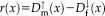
 needs to be specified. This requires the introduction of the underlying imaging model. First, we map both of the description layers into the mid space to obtain an inverse-consistent transformation. Second, we assume heteroskedastic Gaussian noise to account for outliers and perform robust estimation. Third, instead of intensity mapping, we operate on the modality-invariant description layers. This set of assumptions yields the imaging model
 (2)
(2) and variance
 . Note that this model differs from alternative probabilistic approaches [Viola and Wells, 1997; Roche et al., 2000] that consider homoskedastic image noise,
 . To facilitate notation, we define
 for the movable image mapped forward and
 for the fixed image mapped backward. We continue referring to images and description layers as fixed and moving to differentiate between them, although both of them are moving.
 (3)
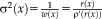
(3) . In fact,
 can be seen as a local weight that determines the influence of the local error. Note that, for a constant variance across the image
 , this reduces to the commonly applied sum of squared differences. The optimization problem changes from estimating just the transformation parameters to additionally estimating the variance at each location

with the vector of variances
 . The joint estimation of transformation parameters and variance can cause a complex optimization problem. We use an iterative optimization procedure that alternates between optimizing the transformation parameters and variances, as summarized in the following Algorithm 1:


end for
Initially, the transformation parameters are set to zero, corresponding to the identity transformation.
1 In step (I), the optimal variances
 are calculated for the transformation of the last iteration
 . In step (II), the optimal transformation
 is calculated for fixed variances
 . An important consequence of the decoupled optimization is that the log-likelihood term in Eq. 3 only depends on the second term when maximizing with respect to the transformation parameters in step (II) of Algorithm 1.
To solve step (I), we draw the relationship to iteratively reweighted least squares estimation for which a large number of robust estimators have been proposed. This allows us to estimate local variances even though we only have a two intensity values at each location
 .
.
Relationship to Iteratively Reweighted Least Squares

 is a symmetric, positive-definite function with a unique minimum at zero and
 . In the following, we concentrate on
 being differentiable, in which case the M-estimator is said to be of
 -type (as
 ). Calculating the derivative yields

 , we obtain
 (4)
(4) (5)
(5) does not depend on the transformation parameter
 , as it is the case for the alternating optimization. Comparing Eqs. 4 and 5, we see that they can be brought into correspondence by identifying
 . This shows that the application of gradient-based optimization for the proposed log-likelihood function is equivalent to the gradient-based optimization of the M-estimator function
 . As the weights are inversely related to the variances, we have
 for different M-estimators
 .
.Robust Estimators
 , for the robust description of the local variances. Here, we specifically model the variances via Tukey's biweight function, as it completely suppresses the effect of outliers:

Figure 2 illustrates Tukey's biweight function as well as the quadratic function with the corresponding weights. The weight function
 for the quadratic function
 is the constant function
 and for Tukey's biweight function is
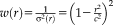 for
for
 and zero otherwise. Tukey's biweight (red curve) limits the influence of large residuals (
 ), for which the weights (red dashed curve) are zero (and the variance infinity). The regular least squares approach (blue curves) results in a constant weight function and variance, independent of the local residuals, and thus considers the contribution of all voxels equally. Using Tukey's estimator requires the saturation parameter
 to be set. A fixed value of
 is recommended for unit Gaussian noise by [Holland and Welsch, 1977; Nestares and Heeger, 2000]. However, it may be more appropriate to specify the value depending on the characteristics of the input images. A method to automatically estimate the saturation parameter for each image pair in a preprocessing step on low-resolution images has been recommended in [Reuter et al., 2010]. The procedure allows for more outliers in the skull, jaw and neck regions, where more variation is to be expected. We use this method to estimate the saturation parameter for entropy images automatically.

Illustration of Tukey's biweight function for
 in red and the quadratic function
 in blue. We also show the corresponding weight function
 as dashed line. The weights are constant for the quadratic function. For Tukey's biweight, the weights are zero for |r|. [Color figure can be viewed in the online issue, which is available at wileyonlinelibrary.com.]
OPTIMIZATION
 (6)
(6) of size
 . As before, the weights do not depend on the transformation parameters
 .
.Steepest descent:

 is the learning rate . Note that the additive update in Lie algebra is equivalent to a compositional update in the Lie group
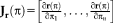
 . The Jacobian
 contains the partial derivatives of all
 parameters, that is,
 with
with

Gauss–Newton and Efficient Second-Order Minimization:


 . The linear approximation yields

 and setting the gradient to zero, leading to the linear system of equations

 . We take a closer look at the Jacobian to see an interesting consequence of the fully symmetric setup

As the first image is mapped exactly in the inverse direction of the second, the derivatives of the transformations only differ by a minus sign. Thus, the transformation derivative
 can be factored out. The resulting formula for the Jacobian is equivalent to the Jacobian of the ESM [Benhimane and Malis, 2004; Vercauteren et al., 2007; Wachinger and Navab, 2009, 2013]. For the fully symmetric registration setup, Gauss–Newton and ESM are therefore equivalent. A similar relationship for another symmetric formulation was independently discovered by [Lorenzi et al., 2013] in an analysis of the log-Demons algorithm.
 for the rigid case [Wachinger and Navab, 2013]


Additional Algorithmic Details
We use a multiresolution approach to estimate large displacements between the images [Roche et al., 1999]. The Gaussian pyramid is constructed by halving each dimension on each level until the image size is approximately
 . This procedure results in five resolution levels for typical image sizes (
 ). The iterations at each level are terminated if the transformation update is below a specified threshold (0.01 mm) or a maximum number of iterations (5) is reached. The registration of the subsequent resolution level is initialized with the result of the previous one.

where
 is the scaling parameter.
2 We choose an exponential intensity scaling, in contrast to square root multiplication of s in [Reuter et al., 2010], because it is symmetric (with respect to the parameter update) and improves the stability of the model.
is the scaling parameter.
2 We choose an exponential intensity scaling, in contrast to square root multiplication of s in [Reuter et al., 2010], because it is symmetric (with respect to the parameter update) and improves the stability of the model.
ENTROPY IMAGES WITH NP WINDOWS
 and a local neighborhood
 , the corresponding description layer is calculated as

with the Shannon entropy
 and
and
 the restriction of the image to the neighborhood
 . The calculation of the local entropy for all locations in the image leads to entropy images. Compared to MI, entropy images have advantages for the registration of images affected by bias fields [Wachinger and Navab, 2012a]. An essential step for the entropy calculation is the estimation of the intensity distribution
 within patches
 . Conversely, the patch size has to be large enough to provide enough samples for reliable density estimation. Conversely, a large patch size leads to smoothing in the images. As we are interested in a highly accurate multimodal registration, we want to reduce the patch size as much as possible to allow for accurate localization and sharp structures.
One approach is to upsample the original image and to utilize the interpolated values for the density estimation. A recently proposed method of NP windows [Dowson et al., 2008] considers the asymptotic case by letting the number of interpolated samples go to infinity. The method involves constructing a continuous space representation of the discrete space signal using a suitable interpolation method. NP windows require only a small number of observed signal samples to estimate the density function and are completely data driven. Originally, Dowson et al. [2008] only presented closed form solutions for certain 1D and 2D density estimation cases. Recently, Joshi et al. [2011] introduced a simplified version of NP windows estimation. Importantly they also include closed form solutions for 3D images. The density is estimated per cube in the volume, where each cube is divided in five tetrahedra. Finding the density estimate over the cube then reduces to finding densities for each of the tetrahedra. We use the NP windows density estimation for entropy images, leading to highly localized entropy images. Figure 3 shows entropy images for density estimation based on histograms and NP windows for different patch sizes. The entropy estimation with NP windows leads to a clear improvement, especially for small patch sizes.

Comparison of entropy images for patch sizes 3 × 3 × 3 to 7 × 7 × 7 created with density estimators based on histogram (a–c) and nonparametric (NP) windows (d–f). Appearance of entropy images is smoother for larger patch sizes. Note the striking difference between the two estimation approaches for patches of size 3 (a vs. d).
EXPERIMENTS
 located at the center of the image. Given two affine transformations in 3D,
 and
and
 , with the
 transformation matrices
 and the
 translation vectors
 , the RMS error is

We calculate the RMS error on transformations in RAS (right, anterior, superior) coordinates, where the origin lies approximately in the center of the image. We set
 mm, to define a sphere that is large enough to include the full brain. For example, an
 error of 0.1 mm corresponds to 1/10 of a voxel displacement (for 1mm isotropic images), which can easily be picked up in visual inspection.
Brain Registration with Ground Truth
In the first experiment, we work with simulated T1 and T2 images from the BrainWeb dataset [Cocosco et al., 1997], which are perfectly aligned. Always knowing the ground truth transformations allows us to establish results on the accuracy of different registration procedures. The image resolution is
 with 1mm isotropic spacing. We automatically skull-strip the T1 image with the BET [Smith, 2002], modify the brain mask (asymmetric and localized dilation), and apply it to the T2 image to induce variations in brain extraction between both modalities. We apply random transformations to the skull-stripped images with translations of 30 mm and rotations around an arbitrary axis of 25°. Different registration approaches are compared to determine how well they recover the correct registration: the statistical analysis of the RMS registration error for 100 repetitions is shown in Figure 4.

Statistical analysis of RMS errors for the skull-strip T1-T2 registration study over 100 repetitions. Bars indicate mean error and correspond to two standard deviations. *** indicates significance level at
 . Robust registration with nonparametric windows (RR-NP) yields a significant reduction in registration error with respect to robust registration with histograms (RR), FLIRT, and SPM. Furthermore, setting the parameter in Tukey's biweight function to
 , which allows for more outliers than
 , yields to significantly better results. [Color figure can be viewed in the online issue, which is available at wileyonlinelibrary.com.]
For the robust registration with NP windows (RR-NP), the patch size is
 and for the robust registration with histograms (RR) it is
 . We manually set the parameter in Tukey's biweight function to simulate a robust approach with many outliers (
 ) and a less robust approach with few outliers (
 ). We compare to popular and freely available registration software using MI: FLIRT in FSL and the coregistration tool in SPM. Our results show the significant reduction in registration error of our approach in contrast to these reference methods. Moreover, we observe a significant improvement for the density estimation with NP windows in comparison to histograms, highlighting the importance of the better localization with NP windows and confirming the qualitative results from Figure 3. Finally, the significant improvement for
 over
over
 demonstrates the necessity for a robust approach to limit the influence of outliers on the registration. The creation of the entropy images took about 9 s with histograms and about 320 s with NP windows. The remaining registration took about 39 s.
Tumor Registration
In the second experiment, we evaluate registration accuracy based on a pair of real brain tumor MR T1 (magnetization-prepared rapid gradient-echo, MPRAGE, [Mugler and Brookeman, 1990]) and MR T2 images, both acquired within the same session. The image resolution is
 mm3 for T1 and isotropic 1 mm for T2. Figure 5 shows the pair of images that we use for the experiments with the corresponding entropy images. Both the automatic skull stripping tool in FreeSurfer and the BET [Smith, 2002] frequently fail for tumor images because of the different appearance of enhancing tumor compared to regular brain tissue, violating intensity priors used by the methods. To produce a useful result, we manually refined the brain extraction obtained from FreeSurfer on the T1 image and propagate the brain mask to the T2 image by registering the full head T1 and T2 images with FLIRT.

Coronal view of full head MR MPRAGE (a) and T2 (b) tumor images with corresponding entropy images (c,d).
When performing robust multimodal registration on the skull-stripped brain images, we expect the tumor regions to be marked as outliers because of the different appearance in both modalities. Figure 6 depicts the weights calculated with Tukey's biweight function (Robust Estimators section) at each spatial location after successful registration. Smaller weights are shown in red and yellow. Note that weights are inversely related to the variances. We observe that tumor regions are marked as outliers (yellow), as expected. Also note the decreased weight at the interface between the brain and the skull, which is likely caused by the inconsistent brain extraction (mask propagation) and differential distortion between the two modalities. These nonmatching structures in tumor regions and artifacts from the brain extraction, that can cause problems for nonrobust techniques, are correctly identified automatically by our method and their influence is limited during the registration.

Coronal view of MR MPRAGE (a) and T2 (b) skull-stripped brain tumor images after registration. Estimated weights are overlaid as heat map. [Color figure can be viewed in the online issue, which is available at wileyonlinelibrary.com.]
In the case of clinical tumor images, we do not know the ground truth alignment. To quantify the registration error, landmarks were manually selected in both modalities, permitting the computation of landmark distances after the registration. Figure 7 shows the statistical analysis for 100 repetitions with the random displacement of the images similar to the previous experiment. We compare RR-NP with patch size 3 to FLIRT and SPM. The results indicate a significantly lower registration error for the proposed RR approach. The manual refinement of the brain extraction and the manual selection of landmarks make the extension of this study to many subjects complicated, but results on a large cohort are presented in the next section.

Statistical analyses of RMS errors for tumor registration study over 100 repetitions. Bars indicate mean error; error bars correspond to two standard deviations. *** indicates significance level at
 . Robust registration with NP windows (RR-NP) yields a significant reduction in registration error. The range of the y-axis is adjusted to highlight the differences of the methods. [Color figure can be viewed in the online issue, which is available at wileyonlinelibrary.com.]
Full Head Registration
In this experiment, we register T1 (Multi-Echo MPRAGE [Kouwe et al., 2008]) and T2 full head images of 106 healthy subjects. These images have a 1 mm isotropic resolution (
 ). Although each image pair was acquired within the same session, we expect local differences caused by jaw, tongue, and small head movements. Such local displacements can deteriorate the registration quality of full head scans. Figure 8 shows a registered pair of T1 and T2 images with an overlay of the estimated weights, together with a magnified view of the area around the tongue. Due to the movement of the tongue between the scans, the RR algorithm detects outliers in that region. Note that also regions in the periphery of the brain show low weights, which are caused by the different appearance of dura mater and CSF in T1- and T2-weighted images. The local information content is different in these regions, yielding differences between the entropy images. The benefit of the robust approach is to identify these contradictory regions as outliers and reduce their influence on the registration.

Sagittal view of MR T1 (a) and T2 (b) full head images with an overlay of the weights as a result of the robust registration. Magnifications of the tongue area (c,d) that is susceptible to motion. Areas with motion differences are assigned low weights to limit their influence on the registration. Also regions in the periphery of the brain are assigned low weights because of the different appearance of CSF and dura mater and resulting dissimilarities in the entropy images. [Color figure can be viewed in the online issue, which is available at wileyonlinelibrary.com.]
Again no ground truth alignment is available, but the number of scans in this study is too large for the manual identification of landmarks. Instead, we assume that the registration of skull-stripped images is more accurate than the registration of the full head images because most structures that are susceptible to patient motion are removed. As both scans were collected within the same session, we do not expect any changes in the brain. Local differences are mainly expected in the scalp, jaw, neck, and eye regions. It is, therefore, reasonable to assume higher registration accuracy when using the brain as a stable region of interest (ROI). Given a reference transformation
 , we compute the RMS error
 , where
 is the transformation computed on the full head scans with registration method Type that we want to evaluate. Figure 9 shows the difference in RMS error between the usage of FLIRT and SPM compared to RR-NP, so
 and
and
 , where positive differences indicate that a better approximation of the reference transformation with RR-NP. To avoid biasing results by selecting only one registration to establish the reference transformation, we report results for using all three registration methods to compute
 , shown on the x-axis of Figure 9. For each subject, we randomly transform the full head images (up to 15° and 20 mm) 10 times and perform the registration with each method, yielding 3180 full head registrations. The results show that RR-NP is significantly better in recovering the reference transformation established on the brain ROI independent of which reference method was used.

Analysis of difference of RMS errors for the large control study on 106 subjects with 10 repeats. The RMS error is computed between full head registrations and the reference transformation, yielding
 , where we use RR-NP, FLIRT, and SPM as registration Type on the full head scans. Differences of RMS errors
 and
and
 are plotted to compare the methods, where positive values show better performance of RR-NP. Bars indicate mean difference error and correspond to standard error of difference. *, **, and *** indicate significance levels from paired t-test at
 ,
,
 and
and
 , respectively. To avoid biasing the results, we use each method (RR-NP, FLIRT, and SPM) to establish the reference transformation on the skull-stripped images (x-axis). [Color figure can be viewed in the online issue, which is available at wileyonlinelibrary.com.]
Histology-OCT Registration
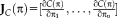
In this multimodal experiment, we register images from OCT with histology slices. OCT is an optical microscopy technique, analogue to ultrasound imaging, which provides a resolution close to 1 µm. This technique requires neither staining nor dyes, as it relies on the intrinsic optical properties of the tissue. The block sample can be imaged prior to any cutting, which greatly reduces the distortions contrary to the histological protocol. Details on the technique and the acquisition of those images can be found in Magnain et al. [2014]. Histology-OCT alignment is of clinical importance to validate the appearance of structures in OCT based on the true appearance on the sliced tissue. The registration is challenging as histology images show artifacts due to local deformations and tearing of the tissues during slicing, which are not present in the previously acquired OCT images. Figure 10 shows the result of the registration between an OCT and histology slice, as well as the estimated weights. The magnified view illustrates the differences between both images and shows that tears in the histology slices are correctly marked as outliers. Figure 11 shows another set of histology and OCT images with the corresponding entropy images. The gyrus was cropped from larger OCT and histology images independently, which introduces small differences at the top boundary edge due to slightly different cropping angles. The weight map shows that these differences together with internal cracks are marked as outliers by the RR.

OCT (first column) and histology (second column) slices together with an overlay of weights on the histology slices (third column). The top row shows the entire slices while the bottom row shows a magnifications around the large crack in the center of the images. Tears in the histology image and alignment errors at the boundary (caused by nonlinear deformations) are marked as outliers. [Color figure can be viewed in the online issue, which is available at wileyonlinelibrary.com.]

OCT (a) and histology (b) slices with corresponding entropy images (c,d). Estimated weights are shown on the OCT slice (e). Outliers are found in cracks of the histology slices and around the boundary. [Color figure can be viewed in the online issue, which is available at wileyonlinelibrary.com.]
To confirm the promising results from the qualitative analysis, we identified 26 landmark correspondences in four histology and corresponding OCT images. We use the transformation from image registration to map the landmarks from the OCT to the histology domain. The average Euclidean distance between mapped OCT and histology landmark pairs measures the registration error. Figure 12 shows the mean and standard error for the RR, for FSL, and for an alternative 2D affine registration method that is based on the SPM algorithm (also using MI and a Powell minimizer). The original SPM registration method is available only for the full 3D case and does not model 2D affine transformations. Because of the high image resolution in our experiment (
 ), we select a larger patch size and the histogram-based density estimation for constructing the entropy images in the RR method. The results from the quantitative analysis confirm the improved registration accuracy of the robust multimodal registration.

Registration error for histology-OCT alignment measured as landmark distance in microns. Results are shown for different registration methods. Bars indicate mean error; error bars correspond to standard error. The range of the y-axis is selected to highlight the differences of the methods. [Color figure can be viewed in the online issue, which is available at wileyonlinelibrary.com.]
Bias Field Robustness
Intensity bias fields in images can severely affect cost functions in cross-modal registration, such as MI [Myronenko and Song, 2010]. On the contrary, the presented approach is very robust with respect to bias fields, as it is based on local entropy estimation. To demonstrate robustness with respect to changes in the bias field, we use five different cases from the BrainWeb dataset [Cocosco et al., 1997] and increase the size of this test set by simulating brain tumors [Prastawa et al., 2009] (including contrast enhancement, local distortion of healthy tissue, infiltrating edema adjacent to tumors, destruction and deformation of fiber tracts). For each of the five original cases, tumor seed were placed at two different locations and two different parameter settings were selected to vary the characteristics of the tumor (conservative vs. aggressive growth), yielding 20 tumor cases. Each simulation produced aligned T1, T2, and T1 Gadolinium enhanced (T1Gad) tumor images (1mm isotropic,
 ) where we added noise and bias fields. We apply random rigid transformations with translations of 30 mm and rotations of 25° around an arbitrary axis with the center of rotation corresponding to the image center, and measure how accurately each test method can estimate the true transformation. We perform the RR for patch sizes between
 and
and
 and again compare to FLIRT and SPM. Figure 13 shows the RMS registration errors for the different cross-modal registration pairs. It can be seen that bias field does not affect the RR approach. SPM performs better than FLIRT, but in both methods registration fails completely in a large number of cases. Without adding a bias field, none of the methods produce any of these severe registration failures (not shown). Bias field correction can, therefore, be expected to remove most of the intensity bias and resulting registration problems, but this additional processing step is not required for our robust entropy-based cross-modal registration approach.

Multimodal registration of 20 synthetic brain tumor images (T1, T2, T1Gad) with bias field. Comparison of RMS errors for different registration methods. Bars indicate mean error; error bars correspond to two standard deviations. White discs correspond to the individual data points. The proposed methods (RR, RR-NP) are robust to bias field due to the local entropy estimation while the bias field has a strong influence on FLIRT and SPM. [Color figure can be viewed in the online issue, which is available at wileyonlinelibrary.com.]
DISCUSSION AND CONCLUSION
We presented a novel registration approach for inverse-consistent, multimodal registration that is robust with respect to local differences and with respect to bias fields. To achieve outlier robustness, we incorporated a heteroskedastic noise model and established the relationship to iteratively reweighed least squares estimation. We derived the Gauss–Newton optimization, which we showed to be equivalent to the ESM in case of our robust and inverse-consistent registration setup. To allow for better localization of structures when constructing entropy images, we used a NP density estimator and demonstrated its advantages. We evaluated our method on different multimodal datasets and demonstrated increased accuracy and robustness. This work focuses on global registration and it remains to investigate the performance and feasibility of the proposed robust multimodal approach for nonlinear registration. One concern is that locations with large differences may be marked as outliers and therefore produce no force on the deformation field, although they could potentially be correctly aligned in subsequent steps. Conversely, deformation fields are never estimated only locally. Regularizers and parametric models combine the forces from several locations. This combination may still push the deformation field in the correct direction, in spite of a reduced weight at certain locations. Adjustments to the robust estimation approach may be required, for instance, the regularization of weights via local smoothing.
The presented registration method will be made freely available within the FreeSurfer software package.
ACKNOWLEDGMENTS
We are very thankful to Niranjan Joshi and Timor Kadir for providing Matlab code of the NP windows estimator. We are very grateful to the unknown reviewers for their insightful comments. BF has a financial interest in CorticoMetrics, a company whose medical pursuits focus on brain imaging and measurement technologies. BF's interests were reviewed and are managed by Massachusetts General Hospital and Partners HealthCare in accordance with their conflict of interest policies.
REFERENCES
- 1 An alternative would be to initialize the transformation based on raw image moments, as described in (Reuter et al., 2010).
- 2 We consider separate noise for fixed and moving image, which are subject to the intensity scaling. Since linear combination of mutually independent normal random variables is again normal distributed, we summarize it into a global noise term.