Classification and image processing with a semi-discrete scheme for fidelity forced Allen–Cahn on graphs
Abstract
This paper introduces a semi-discrete implicit Euler (SDIE) scheme for the Allen-Cahn equation (ACE) with fidelity forcing on graphs. The continuous-in-time version of this differential equation was pioneered by Bertozzi and Flenner in 2012 as a method for graph classification problems, such as semi-supervised learning and image segmentation. In 2013, Merkurjev et. al. used a Merriman-Bence-Osher (MBO) scheme with fidelity forcing instead, as heuristically it was expected to give similar results to the ACE. The current paper rigorously establishes the graph MBO scheme with fidelity forcing as a special case of an SDIE scheme for the graph ACE with fidelity forcing. This connection requires the use of the double-obstacle potential in the ACE, as was already demonstrated by Budd and Van Gennip in 2020 in the context of ACE without a fidelity forcing term. We also prove that solutions of the SDIE scheme converge to solutions of the graph ACE with fidelity forcing as the discrete time step converges to zero. In the second part of the paper we develop the SDIE scheme as a classification algorithm. We also introduce some innovations into the algorithms for the SDIE and MBO schemes. For large graphs, we use a QR decomposition method to compute an eigendecomposition from a Nyström extension, which outperforms the method used by, for example, Bertozzi and Flenner in 2012, in accuracy, stability, and speed. Moreover, we replace the Euler discretization for the scheme's diffusion step by a computation based on the Strang formula for matrix exponentials. We apply this algorithm to a number of image segmentation problems, and compare the performance with that of the graph MBO scheme with fidelity forcing. We find that while the general SDIE scheme does not perform better than the MBO special case at this task, our other innovations lead to a significantly better segmentation than that from previous literature. We also empirically quantify the uncertainty that this segmentation inherits from the randomness in the Nyström extension.
1 INTRODUCTION
- the MBO scheme with fidelity forcing is a special case of the SDIE scheme with fidelity forcing; and
- the SDIE solution converges to the solution of Allen-Cahn with fidelity forcing as the SDIE time step tends to zero.
We then demonstrate how to employ the SDIE scheme as a classification algorithm, making a number of improvements upon the MBO-based classification in 32. In particular, we have developed a stable method for extracting an eigendecomposition or singular value decomposition (SVD) from the Nyström extension 21, 36 that is both faster and more accurate than the previous method used in 6, 32. Finally, we test the performance of this scheme as an alternative to graph MBO as a method for image processing on the “two cows” segmentation task considered in 6, 32.
Given an edge-weighted graph, the goal of two-class graph classification is to partition the vertex set into two subsets in such a way that the total weight of edges within each subset is high and the weight of edges between the two subsets is low. Classification differs from clustering by the addition of some a priori knowledge, that is, for certain vertices the correct classification is known beforehand. Graph classification has many applications, such as semi-supervised learning and image segmentation 6, 15.
All programming for this paper was done in Matlab R2019a. Except within algorithm environments and URLs, all uses of typewriter font indicate built-in Matlab functions.
1.1 Contributions of this work
- Defined a double-obstacle ACE with fidelity forcing (Definition 2.6), and extended the theory of 13 to this equation (Theorem 2.7).
- Defined an SDIE scheme for this ACE (Definition 2.8) and following 13 proved that this scheme is a generalization of the fidelity forced MBO scheme (Theorem 2.9), derived a Lyapunov functional for the SDIE scheme (Theorem 2.12), and proved that the scheme converges to the ACE solution as the time-step tends to zero (Theorem 2.17).
- Described how to employ the SDIE scheme as a generalization of the MBO-based classification algorithm in 32.
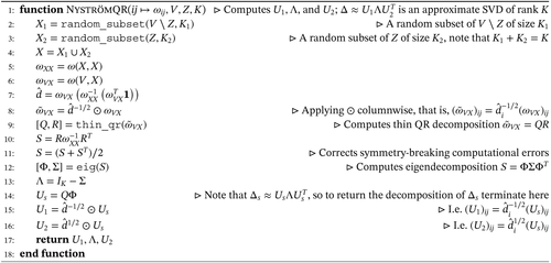
- Developed a method, inspired by 3, using the QR decomposition to extract an approximate SVD of the normalized graph Laplacian from the Nyström extension (Algorithm 1), which avoids the potential for errors in the method from 6, 32 that can arise from taking the square root of a non-positive-semi-definite matrix, and empirically produces much better performance than the 6, 32 method (Figure 4) in accuracy, stability, and speed.
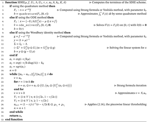
- Developed a method using the quadratic error Strang formula for matrix exponentials 39 for computing fidelity forced graph diffusion (Algorithm 2), which empirically incurs a lower error than the error incurred by the semi-implicit Euler method used in 32 (Figure 6), and explored other techniques with the potential to further reduce error (Table 1).
- Demonstrated the application of these algorithms to image segmentation, particularly the “two cows” images from 6, 32, compared the quality of the segmentation to those produced in 6, 32 (Figure 11), and investigated the uncertainty in these segmentations (Figure 14), which is inherited from the randomization in Nyström.
| Relative ℓ2 error for | Relative ℓ2 error for | |||||
|---|---|---|---|---|---|---|
| Method | |V|=1600, K = 1600 | |V|=1600, K = 40 | |V|=6400, K = 40 | |V|=1600, K = 1600 | |V|=1600, K = 40 | |V|=6400, K = 40 |
| Semi-implicit Euler 32 | 1.434 × 10⁻⁴ | 0.4951 | 0.4111 | 2.882 × 10⁻⁴ | 0.2071 | 0.1721 |
| Woodbury identity | 2.292 × 10⁻⁸ | 0.5751 | 0.4607 | 1.038 × 10⁻⁷ | 0.1973 | 0.1537 |
| Midpoint rule (3.3) | 0.0279 | 0.1290 | 0.1110 | 0.4279 | 0.6083 | 0.6113 |
| Simpson's rule (m = 500) via Strang formula | 2.592 × 10⁻⁹ | 0.1335 | 0.1136 | 5.845 × 10⁻⁷ | 0.5124 | 0.4827 |
| Matlab integrate via Strang formula | n/a | 0.1335 | 0.1136 | n/a | 0.5124 | 0.4827 |
| Simpson's rule (m = 500) via Yoshida method | 8.381 × 10⁻¹⁴ | 0.1335 | 0.1136 | 9.335 × 10⁻¹² | 0.5124 | 0.4827 |
| Matlab integrate via Yoshida method | n/a | 0.1335 | 0.1136 | n/a | 0.5124 | 0.4827 |
- Note: We did not compute integrate for K = 1600 as it ran too slowly. Bold entries indicate the smallest error in that column.
This work extends the work in 13 in four key ways. First, introducing fidelity forcing changes the character of the dynamics, for example, making graph diffusion affine, which changes a number of results/proofs, and it is thus of interest that the SDIE link continues to hold between the MBO scheme and the ACE. Second, this work for the first time considers the SDIE scheme as a tool for applications. Third, in developing the scheme for applications we have made a number of improvements to the methods used in the previous literature 32 for MBO-based classification, which result in a better segmentation of the “two cows” image than that produced in 32 or 6. Fourth, we quantify the randomness that the segmentation inherits from the Nyström extension.
1.2 Background
In the continuum, a major class of techniques for classification problems relies upon the minimization of total variation (TV), for example, the famous Mumford-Shah 34 and Chan-Vese 16 algorithms. These methods are linked to Ginzburg-Landau methods by the fact that the Ginzburg-Landau functional -converges to TV 29, 33 (a result that continues to hold in the graph context 23). This motivated a common technique of minimizing the Ginzburg-Landau functional in place of TV, for example, in 20 two-class Chan-Vese segmentation was implemented by replacing TV with the Ginzburg-Landau functional; the resulting energy was minimized by using a fidelity forced MBO scheme.
In 32 an alternative method was introduced: a graph MBO scheme with fidelity forcing. The original MBO scheme, introduced in a continuum setting in 4 to approximate motion by mean curvature, is an iterative scheme consisting of diffusion alternated with a thresholding step. In 32 this scheme was discretized for use on graphs and the fidelity forcing term (where M is a diagonal nonnegative matrix, see Section 2 for details) was added to the diffusion. Heuristically, this MBO scheme was expected to behave similarly to the graph ACE as the thresholding step resembles a “hard” version of the “soft” double-well potential nonlinearity in the ACE.
In 13 it was shown that the graph MBO scheme without fidelity forcing could be obtained as a special case of a SDIE scheme for the ACE (without fidelity forcing), if the smooth double-well potential was replaced by the double-obstacle potential defined in (1.2), and that solutions to the SDIE scheme converge to the solution of the graph ACE as the time step converges to zero. This double-obstacle potential was studied for the continuum ACE in 8-10 and was used in the graph context in 11. In 14 a result similar to that of 13 was obtained for a mass-conserving graph MBO scheme. In this paper such a result will be established for the graph MBO scheme with fidelity forcing.
In 24 it was shown that the graph MBO scheme pins (or freezes) when the diffusion time is chosen too small, meaning that a single iteration of the scheme will not introduce any change as the diffusion step will not have pushed the value at any node past the threshold. In 13 it was argued that the SDIE scheme for graph ACE provides a relaxation of the MBO scheme: the hard threshold is replaced by a gradual threshold, which should allow for the use of smaller diffusion times without experiencing pinning. The current paper investigates what impact that has in practical problems.
1.3 Groundwork
Finally, we recall some notation from 13: for problems of the form we write f ≃ g and say f and g are equivalent when g(x) = af(x) + b for a > 0 and b independent of x. As a result, replacing f by g does not affect the minimizers.
Lastly, we define the non-fidelity-forced versions of the graph MBO scheme, the graph ACE, and the SDIE scheme.
- , that is, the diffused state of un after a time .
- where is defined by, for all i ∈ V and ,
()
- When , this scheme is exactly the MBO scheme.
- For ε fixed and , this scheme converges to the solution of the double-obstacle ACE (which is a well-posed ODE).
1.4 Paper outline
The paper is structured as follows. In Section 1.3 we introduced important concepts and notation for the rest of the paper. Section 2 contains the main theoretical results of this paper. It defines the graph MBO scheme with fidelity forcing, the graph ACE with fidelity forcing, and the SDIE scheme for graph ACE with fidelity forcing. It proves well-posedness for the graph ACE with fidelity forcing and establishes the rigorous link between a particular SDIE scheme and the graph MBO with fidelity forcing. Moreover, it introduces a Lypunov functional for the SDIE scheme with fidelity forcing and proves convergence of solutions of the SDIE schemes to the solution of the graph ACE with fidelity forcing. In Section 3 we explain how the SDIE schemes can be used for graph classification. In particular, the modifications to the existing MBO-based classification algorithms based on the QR decomposition and Strang formula are introduced. Section 4 presents a comparison of the SDIE and MBO scheme for image segmentation applications, and an investigation of the uncertainty in these segmentations. In Appendix A it is shown that the application of the Euler method used in 32 can be seen as an approximation of the Lie product formula.
2 THE ACE, THE MBO SCHEME, AND THE SDIE SCHEME WITH FIDELITY FORCING
2.1 The MBO scheme with fidelity forcing
Following 20, 32, we introduce fidelity forcing into the MBO scheme by first defining a fidelity forced diffusion.
Definition 2.1. (Fidelity forced graph diffusion)For and we define fidelity forced diffusion to be:
Note.This fidelity term generalizes slightly the one used (for ACE) in 6, in which for a parameter (ie, fidelity was enforced with equal strength on each vertex of the reference data) yielding where PZ is the projection map:
Proposition 2.2.A is invertible with .
Proof.For the lower bound, we show that A is strictly positive definite. Let u ≠ 0 be written for v ⊥ 1. Then
Theorem 2.3.For given , (2.1) has a unique solution in . The solution u to (2.1) is and is given by the map (where I denotes the identity matrix):
-
If u0 ≤ v0 vertexwise, then for all t ≥ 0, vertexwise.
-
for all t ≥ 0, that is, if then .
Proof.It is straightforward to check directly that (2.2) satisfies (2.1) and is C1 on (0, ∞). Uniqueness is given by a standard Picard-Lindelöf argument (see eg, [40, Corollary 2.6]).
-
By definition, . Thus it suffices to show that e−tA is a nonnegative matrix for t ≥ 0. Note that the off-diagonal elements of −tA are nonnegative: for i ≠ j, . Thus for some a > 0, Q ≔ aI − tA is a nonnegative matrix and thus eQ is a nonnegative matrix. It follows that e−tA = e−aeQ is a nonnegative matrix.
-
Let and recall that . Suppose that for some t > 0 and some i ∈ V, ui(t) < 0. Then
and since each ui is continuous this minimum is attained at some t∗ ∈ [0, t] and i∗ ∈ V. Fix such a t∗. Then for any i∗ minimizing u(t∗), since we must have t∗ > 0, so is differentiable at t∗ with . However by (2.1)We claim that we can choose a suitable minimizer i∗ such that this is strictly positive. First, since any such i∗ is a minimizer of u(t∗), and for all i, it follows that each term is nonnegative. Next, suppose such an i∗ has a neighbor j such that , then it follows that and we have the claim. Otherwise, all the neighbors of that i∗ are also minimizers of u(t∗). Repeating this same argument on each of those, we either have the claim for the above reason or we find a minimizer i∗ ∈ Z, since G is connected. But in that case , since is strictly positive on Z, and we again have the claim. Hence , a contradiction. Therefore ui(t) ≥ 0 for all t. The case for ui(t) ≤ 1 is likewise.
Definition 2.4. (Graph MBO with fidelity forcing)For we follow 20, 32, and define the sequence of MBO iterates by diffusing with fidelity for a time and then thresholding, that is
2.2 The ACE with fidelity forcing
Theorem 2.5.Let obey (2.6) at a.e. t ∈ T, with . Then for all i ∈ V and a.e. t ∈ T,
Proof.Follows as in [13, Theorem 2.2] mutatis mutandis.
Thus following 13 we define the double-obstacle ACE with fidelity forcing.
Definition 2.6. (Double-obstacle ACE with fidelity forcing)Let T be an interval. Then a pair is a solution to double-obstacle ACE with fidelity forcing on T when and for almost every t ∈ T,
We now demonstrate that this has the same key properties, mutatis mutandis, as the ACE in 13.
Theorem 2.7.Let T = [0, T0] or [0, ∞). Then:
-
(Existence) For any given , there exists a as in Definition 2.6 with u(0) = u0.
-
(Comparison principle) If with satisfy
()and()vertexwise at a.e. t ∈ T, and v(0) ≤ u(0) vertexwise, then v(t) ≤ u(t) vertexwise for all t ∈ T. -
(Uniqueness) If and are as in Definition 2.6 with u(0) = v(0) then u(t) = v(t) for all t ∈ T and at a.e. t ∈ T.
-
(Gradient flow) For u as in Definition 2.6, monotonically decreases.
-
(Weak form) (and associated a.e.) is a solution to (2.8) if and only if for almost every t ∈ T and all
() -
(Explicit form) satisfies Definition 2.6 if and only if for a.e. t ∈ T, , and (for B ≔ A − ε−1I and ):
() -
(Lipschitz regularity) For u as in Definition 2.6, if , then .
-
(Well-posedness) Let define the ACE trajectories u, v as in Definition 2.6, and suppose . Then, for ,
()
Proof.
-
We prove this as Theorem 2.17.
-
We follow the proof of [13, Theorem B.2]. Letting w ≔ v − u and subtracting (2.9) from (2.10), we have that
vertexwise at a.e. t ∈ T. Next, take the inner product with , the vertexwise positive part of w:As in the proof of [13, Theorem B.2], the RHS ≤ 0. For the rest of the proof to go through as in that theorem, it suffices to check that ⟨Aw(t), w+(t)⟩ ≥ ⟨Aw+(t), w+(t)⟩. But by [13, Proposition B.1], , and ⟨Mw(t), w+(t)⟩ = ⟨Mw+(t), w+(t)⟩ since M is diagonal, so the proof follows as in [13, Theorem B.2]. -
Follows from (b): if and have u(0) = v(0) and both solve (2.8), then applying the comparison principle in both directions gives that u(t) = v(t) at all t ∈ T. Then (2.7) gives that at a.e. t ∈ T.
-
We prove this in Theorem 2.20 for the solution given by Theorem 2.17, which by uniqueness is the general solution.
-
Let u solve (2.8). Then for a.e. t ∈ T, , and at such t we have for all as in the proof of [13, Theorem 3.8], so u satisfies (2.11). Next, if u satisfies (2.11) at t ∈ T, then as in the proof of [13, Theorem 3.8], , as desired.
-
Let . If: We check that (2.12) satisfies (2.8). Note first that we can rewrite (2.8) as
Next, let u be as in (2.12). Then it is easy to check thatand that this satisfies (2.8). Next, we check the regularity of u. The continuity of u is immediate, as it is a sum of two smooth terms and the integral of a locally bounded function. To check that : u is bounded, so is locally L2, and by above du/dt is a sum of (respectively) two smooth functions, a bounded function and the integral of a locally bounded function, so is locally bounded and hence locally L2.Only if: We saw that (2.12) solves (2.8) with and , and by (c) such solutions are unique.
-
We follow the proof of [13, Theorem 3.13]. Let 0 ≤ t1 < t2. Since (2.8) is time-translation invariant, we have by (f) that
and so, writing Bs ≔ (e−sB − I)/s for s > 0 (which we note commutes with B),Note that Bs is self-adjoint, and as −B has largest eigenvalue less than ε−1 we have ||Bs||< (es/ε − 1)/s, with RHS monotonically increasing in s for s > 0.1Since and for all t, and , we have for t2 − t1 < 1:and for t2 − t1 ≥ 1 we simply havecompleting the proof. -
We prove this as Theorem 2.21 for the solution given by Theorem 2.17, which by uniqueness is the general solution.
Note.Given the various forward references in the above proof, we take care to avoid circularity by not using the corresponding results until they have been proven.
2.3 The SDIE scheme with fidelity forcing and link to the MBO scheme
Definition 2.8. (SDIE scheme with fidelity forcing, cf. [[13], Definition 4.1])For , , and we define the SDIE scheme iteratively:
As in 13, we have the key theorem linking the MBO scheme and the SDIE schemes for the ACE.
Theorem 2.9. (Cf. [[13], Theorem 4.2])For , the pair is a solution to the SDIE scheme (2.14) for some if and only if un + 1 solves:
Proof.Identical to the proof of [13, Theorem 4.2] with the occurrences of “” in each instance replaced by “.”
As in [13, Figure 1], we can plot (2.16) to visualize the SDIE scheme (2.14) as a piecewise linear relaxation of the MBO thresholding rule. Next, we note that we have the same Lipschitz continuity property from [13, Theorem 4.4].

Theorem 2.10. (Cf. [[13], Theorem 4.4])For 2and all , if un and vn are defined according to Definition 2.8 with initial states and then
Proof.Follows as in [13, Theorem 4.4] mutatis mutandis.
2.4 A Lyapunov functional for the SDIE scheme
Lemma 2.11. (Cf. [[24], Lemma 4.6])The functional on
-
It is strictly concave.
-
It has first variation at u
Proof.Let . We expand around u:
-
for v ≠ 0.
-
Since e−tA is self-adjoint, .
Theorem 2.12. (Cf. [[13], Theorem 4.9])For we define on the functional
Proof.We can rewrite H as:
Corollary 2.13.For (ie, the MBO case) the sequence un defined by (2.14) is eventually constant.
For , the sum
2.5 Convergence of the SDIE scheme with fidelity forcing
Following 13, we first derive the nth term for the semi-discrete scheme.
Proposition 2.14. (Cf. [[13], Proposition 5.1])For the sake of notation, define:
Proof.We can rewrite (2.14) as
Next, we consider the asymptotics of each term in (2.22).
Theorem 2.15.Considering relative to the limit of and n → ∞ with for some fixed t ≥ 0 and for fixed ε > 0 (with )4, and recalling that , B ≔ A − ε−1I and :
-
.
-
.
-
.
Hence by (2.22), the SDIE term obeys
Proof.Let . Note that for any bounded matrix X.
Note that is the same as , and also that, for bounded (in ) invertible matrices X and Y with bounded (in ) inverses, if and only if .5
-
, so it suffices to consider . Since we infer that
-
We note that
We next consider each term of w individually. First, we seek to show thatso it suffices to show thatThis holds if and only ifand since B = A − ε−1I the result follows. Next we seek to show thatso it suffices to show thatwhich holds if and only ifand since B = A − ε−1I the result follows. -
We follow [13, Proposition 5.1] and consider the difference
as desired.
Theorem 2.16.For any sequence with for all n, there exists a function and a subsequence such that converges weakly to z in . It follows that:
- (A)
in , where .
- (B)
For all t ≥ 0,
- (C)
Passing to a further subsequence of , we have strong convergence of the Cesàro sums, that is, for all bounded T ⊆ [0, ∞)
as N → ∞.
-
for all t ≥ 0,
-
, and
-
for a.e. t ≥ 0.
These results follow as in 13. Item (a) follows immediately from the fact that for all n, .
Theorem 2.17. (Cf. [[13], Theorem 5.4])For any given , ε > 0 (with ) and , there exists a subsequence of with for all n, along which the SDIE iterates given by (2.14) with initial state u0 converge to the ACE solution with initial condition u0 in the following sense: For each t ≥ 0, as n → ∞ and , , and there is a sequence Nk → ∞ such that for almost every t ≥ 0, , where is the solution to (2.8) with .
Corollary 2.18.Let , ε > 0, , and with for all n. Then for each t ≥ 0, as n → ∞, .
Proof.Let and let be any subsequence of . Then by the theorem there is a subsubsequence such that pointwise where is a solution to (2.8) with initial condition . By Theorem 2.7(c) such solutions are unique, so . Thus there exists x (in particular, ) such that every subsequence of xn has a convergent subsubsequence with limit x. It follows by a standard fact of topological spaces that pointwise as n → ∞.6
Finally, we follow 13 to use Theorem 2.17 to deduce that the Ginzburg-Landau energy monotonically decreases along the ACE trajectories by considering the Lyapunov functional H defined in (2.19). We also deduce well-posedness of the ACE.
Proposition 2.19. (Cf. [[13], Proposition 5.6])Let . Then for
Proof.Expanding and collecting terms in (2.5), we find that for
Theorem 2.20. (Cf. [[13], Theorem 5.7, Remark 5.8])Suppose and . Then the ACE trajectory u defined by Definition 2.6 has monotonically decreasing in t. More precisely: for all t > s ≥ 0,
Theorem 2.21. (Cf. [[13], Theorem 3.11])Let define ACE trajectories u, v by Definition 2.6, and suppose . Then, if , then
3 THE SDIE SCHEME AS A CLASSIFICATION ALGORITHM
As was noted in the introduction, trajectories of the ACE and of the MBO scheme on graphs can be deployed as classification algorithms, as was originally done in work by Bertozzi and coauthors in 6, 32. In the above, we have shown that the SDIE scheme (2.14) introduced in 13 generalizes the MBO scheme into a family of schemes, all of the same computational cost as the MBO scheme, and which as become increasingly more accurate approximations of the ACE trajectories. In the remainder of this paper, we will investigate whether the use of these schemes can significantly improve on the use of the MBO scheme to segment the “two cows” images from 6, 32. We will also discuss other potential improvements to the method of 32.
3.1 Groundwork
In this section, we will describe the framework for applying graph dynamics to classification problems, following 6, 32.
The individuals that we seek to classify we will denote as a set V, upon which we have some information . For example, in image segmentation V is the pixels of the image, and x is the grayscale/RGB/etc values at each pixel. Furthermore, we have labeled reference data which we shall denote as Z ⊆ V and binary reference labels supported on Z. Supported on Z we have our fidelity parameter , and we recall the notation and (recall that the operator diag sends a vector to the diagonal matrix with that vector as diagonal, and also vice versa).
To build our graph, we first construct feature vectors . The philosophy behind these is that we want vertices which are “similar” (and hence should be similarly labeled) to have feature vectors that are “close together.” What this means in practice will depend on the application, for example, 41 incorporates texture into the features and 6, 15 give other options.
3.2 The basic classification algorithm
- Input: Vector , reference data Z, and labels f supported on Z.
- Convert x into feature vectors .
- Build a weight matrix on V2 via .
- Compute A and therefore b.
- From some initial condition u0, compute the SDIE sequence un until it meets a stopping condition at some n = N.
- Output: uN thresholded to lie in , that is, we output where is as in (1.1).
Unfortunately, as written this algorithm cannot be feasibly run. The chief obstacle is that in many applications A is too large to store in memory, yet we need to quickly compute , potentially a large number of times. We also need to compute b accurately . Moreover, in general A does not have low numerical rank, so it cannot be well approximated by a low-rank matrix. In the rest of this section we describe our modifications to this basic algorithm that make it computationally efficient.
3.3 Matrix compression and approximate SVDs
Following 6, 32, we next compute an approximate eigendecomposition of . We here diverge from the method of 6, 32. The method used in those papers requires taking the matrix square root of , but unless is the zero matrix it will not be positive semi-definite.7While this clearly does not prevent the method of 6, 32 from working in practice, it is a potential source of error and we found it conceptually troubling. We here present an improved method, adapted from the method from 3 for computing a SVD from an adaptive cross approximation (ACA) (see 3 for a definition of ACA).
Algorithm 1. QR decomposition-based Nyström method for computing an approximate SVD of , inspired by [3].
3.3.1 Numerical assessment of the matrix compression method
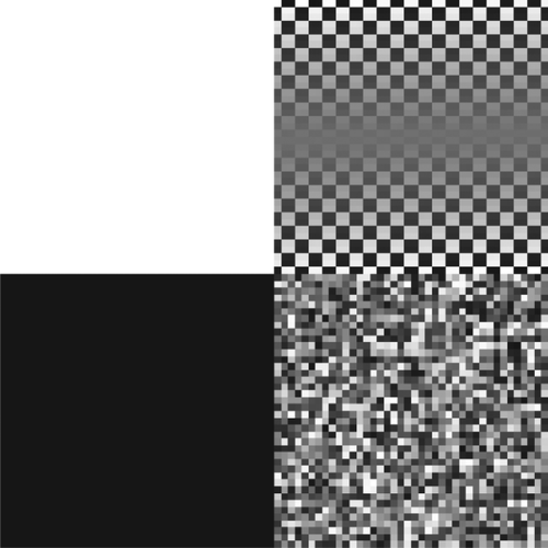
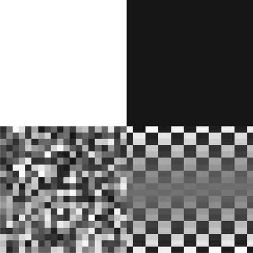
We consider the accuracy of our Nyström-QR approach for the compression of the symmetric normalized Laplacian8 built on the simple image in Figure 3, containing |V| = 6400 pixels, which is small enough for us to compute the true value of to high accuracy. For K ∈ {50, 100, ⋯ , 500}, we compare the rank K approximation with the true in terms of the relative Frobenius distance, that is, . Moreover, we compare these errors to the errors incurred by other low-rank approximations of , namely the Nyström method used in 6, 32, the Halko-Martinsson-Tropp (HMT) method9 26, and the optimal rank K approximation of with respect to || · ||F, which (by the Eckart-Young theorem 19; see also [25, Theorem 2.4.8]) is obtained by setting all but the K leading singular values of to 0. In addition to the methods' accuracy, we measure their complexity via the runtimes of Matlab R2019a implementations of them on the set-up as in Section 4.2.
We report the relative Frobenius distance in Figure 4. As the Nyström (and HMT) methods are randomized, we repeat the experiments 1000 times and plot the mean error in the far-left figure and the standard deviations in the center-right figure. To expose the difference between the methods for K ≥ 100, we plot the percentage increase of the other errors above the SVD error (ie, [error/errorSVD − 1] × 100%) and show this percentage in the center-left figure. In the far-right figure, we compare the complexity of the algorithms in terms of their average runtime. The SVD timing is constant in K as we always computed a full SVD and kept the largest K singular values.

We observe that the Nyström-QR method outperforms the Nyström method from 6, 32: it is faster, more accurate, and is stable for small K. In terms of accuracy, the Nyström-QR error is only about 0.012% larger than the optimal low-rank error. Notably, this additional error is (almost) constant, indicating that the Nyström-QR method and the SVD converge at a similar rate. The Nyström-QR randomness has hardly any effect on the error; the standard deviation of the relative error ranges from 8.87 × 10⁻⁷ (K = 50) to 5.00 × 10⁻⁸ (K = 500). By contrast, for the Nyström method from 6, 32 we see much more random variation. The bump in the HMT error at K = 450 is an outlier that is present (though not always for the same K) in many repeats of this experiment.
3.4 Implementing the SDIE scheme: a Strang formula method
To compute the iterates of our SDIE scheme, we will need to compute an approximation for . In 32, at each iteration was approximated via a semi-implicit Euler method, which therefore incurred a linear (in the time step of the Euler method, that is, in the below notation) error in both the and b terms (plus a spectrum truncation error). In Appendix A1 we show that the method from 32 works by approximating a Lie product formula approximation (see [27, Theorem 2.11]) of , therefore we propose as an improvement a scheme that directly employs the superior Strang formula10 to approximate —with quadratic error (plus a spectrum truncation error). We also consider potential improvements of the accuracy of computing b: by expressing b as an integral and using quadrature methods11; by expressing b as a solution to the ODE from (2.1) with initial condition 0, and using the Euler method from 32 with a very small time step (or a higher-order ODE solver)12; or by computing the closed form solution for b directly using the Woodbury identity. We therefore improve on the accuracy of computing at low cost.
Given these ingredients, it is then straightforward to compute the SDIE scheme sequence via Algorithm 2.
3.4.1 Numerical assessment of methods
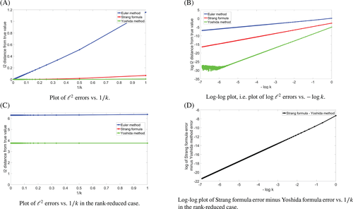
In this section, we will build our graphs on the image in Figure 5, which is small enough for us to compute the true values of (with A here given by ) and b to high accuracy. First, in Figure 6 we investigate the accuracy of the Strang formula and Yoshida method vs the 32 Euler method. We take |V|=1600, , u a random vector given by Matlab's rand(1600,1), and as the characteristic function of the left two quadrants of the image. We consider two cases: one where K = |V| (ie, full-rank) and one where . We observe that the Strang formula and Yoshida method are more accurate than the Euler method in both cases, and that the Yoshida method is more accurate than the Strang formula, but only barely in the rank-reduced case. Furthermore, the log-log gradients of the Strang formula error and the Yoshida method error (excluding the outliers for small k values and the outliers caused by errors from reaching machine precision) in Figure 6(b) are respectively 2.000 and 3.997 (computed using polyfit), confirming that these methods achieve their theoretical orders of error in the full-rank case.
Next, in Table 1 we compare the accuracy of the different methods for computing b. We take Z as the left two quadrants of the image, , as equal to the image on Z, and kb = 1000 in the Strang formula/Yoshida method approximations for e−tAf and in the 32 Euler scheme. We observe that the rank reduction plays a significant role in the errors incurred, and that no method is hands-down superior. In the “two cows” application (Example 4.1), we have observed that (interestingly) the 32 Euler method yields the best segmentation. A topic for future research can be whether this is generally true for large matrices.
4 APPLICATIONS IN IMAGE PROCESSING
4.1 Examples
We consider three examples, all using images of cows from the Microsoft Research Cambridge Object Recognition Image Database (available at https://www.microsoft.com/en-us/research/project/image-understanding/15). Some of these images have been used before by 6, 32 to illustrate and test graph-based segmentation algorithms.
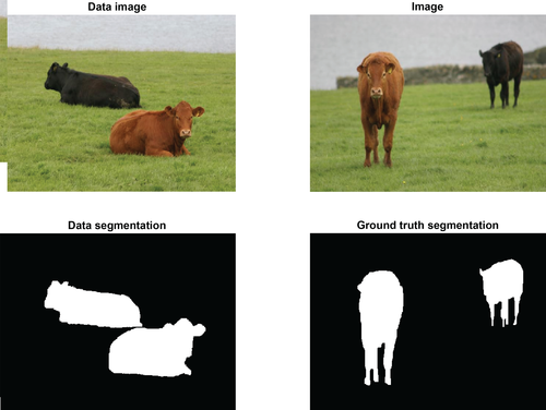
Example 4.1. (Two cows)We first introduce the two cows example familiar from 6, 32. We take the image of two cows in the top left of Figure 7 as the reference data Z and the segmentation in the bottom left as the reference labels , which separate the cows from the background. We apply the SDIE scheme to segment the image of two cows shown in the top right of Figure 7, aiming to separate the cows from the background, and compare to the ground truth in the bottom right. Both images are RGB images of size 480 × 640 pixels, that is, the reference data and the image are tensors of size 480 × 640 × 3.
- study the influence of the parameters ε and , comparing non-MBO SDIE () and MBO SDIE ();
- compare different normalizations of the graph Laplacian, that is, the symmetric vs random walk normalization;
- investigate the influence of the Nyström-QR approximation of the graph Laplacian in terms of the rank K; and
- quantify the inherent uncertainty in the computational strategy induced by the randomized Nyström approximation.
Example 4.2. (Grayscale)This example is the grayscale version of Example 4.1. Hence, we map the images in Figure 7 to grayscale using rgb2gray. We show the grayscale images in Figure 8. We use the same segmentation of the reference data image as in Example 4.1. The grayscale images are matrices of size 480 × 640.
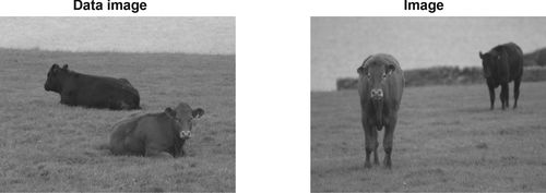
The grayscale image is much harder to segment than the RGB image, as there is no clear color separation. With Example 4.2, we aim to illustrate the performance of the SDIE scheme in a harder segmentation task.
Example 4.3. (Many cows)In this example, we have concatenated four images of cows that we aim to segment as a whole. We show the concatenated image in Figure 9. Again, we shall separate the cows from the background. As reference data, we use the reference data image and labels as in Example 4.1. Hence, the reference data is a tensor of size 480 × 640 × 3. The image consists of approximately 1.23 megapixels. It is represented by a tensor of size 480 × 2560 × 3.

With Example 4.3, we will illustrate the application of the SDIE scheme to large scale images, as well as the case where the image and reference data are of different sizes.
Note.In each of these examples we took as reference data a separate reference data image. However, our algorithm does not require this, and one could take a subset of the pixels of a single image to be the reference data, and thereby investigate the impact of the relative size of the reference data on the segmentation, which is beyond the scope of this paper but is explored for the 32 MBO segmentation algorithm and related methods in [37, Figure 4].
4.2 Set-up
AlgorithmsWe here use the Nyström-QR method to compute the rank K approximation to the Laplacian, and we use the 32 semi-implicit Euler method (with time step ) to compute b (as we found that in practice this worked best for the above examples).
Interpolation sets For the interpolation sets X1, X2 in Nyström we took K1 = K2 = K/2. That is, we took K/2 vertices from the reference data image and K/2 vertices from the image to be segmented, chosen at random using randperm. We experimented with choosing interpolation sets using ACA (see 3), but this showed no improvement over choosing random sets, and ran much slower.
Initial condition We took the initial condition, that is, u0, to equal the reference on the reference data vertices and to equal 0.49 on the vertices of the image to be segmented (where labels “cow” with 1 and “not cow” with 0). We used 0.49 rather than the more natural 0.5 because the latter led to much more of the background (eg, the grass) getting labeled as “cow.” This choice can be viewed as incorporating the slight extra a priori information that the image to be segmented has more non-cow than cow.
Note.It is not an improvement to initialize with the exact proportion of cow in the image (about 0.128), as in that case the thresholding is liable to send every ui for i ∈ V ∖ Z to zero. If one has access to that a priori information, one should use such an initial condition alongside a mass-conserving scheme. We investigate a semi-discrete scheme for mass-conserving Allen-Cahn (without fidelity forcing) in 14, which can be extended to the fidelity-forced case in a manner similar to that of this paper. What the 0.49 initial condition does is more modest. After the initial diffusion, some pixels will have a value very close to 0.5; by lowering the value of the initial condition, we lower the diffused values, introducing a bias towards classifying these borderline pixels as “not cow.” As there is more non-cow than cow in the image, this bias improves the accuracy. It is unknown to the authors why this was necessary for us but was not necessary for 32 nor for 6.
Fidelity parameterWe followed 32 and took , for a parameter.
Computational set-up All programming was done in Matlab R2019a with relevant toolboxes the Computer Vision Toolbox Version 9.0, Image Processing Toolbox Version 10.4, and Signal Processing Toolbox Version 8.2. All reported runtimes are of implementations executed serially on a machine with an Intel® Core™ i7-9800X @ 3.80 GHz [16 cores] CPU and 32 GB RAM of memory.
4.3 Two cows
We begin with some examples of segmentations obtained from the SDIE scheme. Based on these, we illustrate the progression of the algorithm and discuss the segmentation output qualitatively. We will give a quantitative analysis in Section 4.3.1. Note that we give here merely typical realizations of the random output of the algorithm—the output is random due to the random choice of interpolation sets in the Nyström approximation. We investigate the stochasticity of the algorithm in Section 4.3.2.
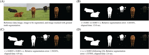
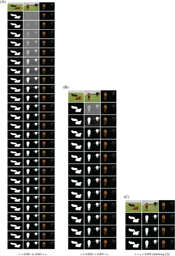
We consider three different cases: the MBO case and two non-MBO cases, where , and . We show the resulting reconstructions from these methods in Figure 10. Moreover, we show the progression of the algorithms in Figure 12. The parameters not given in the captions of Figure 10 are , , kb = 1, k = 1, , and K = 70.
Note.The regime is not of much interest since, by [13, Remark 4.8] mutatis mutandis, in this regime the SDIE scheme has nonunique solution for the update, of which one is just the MBO solution.
Comparing the results in Figure 10, we see roughly equivalent segmentations and segmentation errors. Indeed, the cows are generally nicely segmented in each of the cases. However, the segmentation also labels as “cow” a part of the wall in the background and small clumps of grass, while a small part of the left cow's snout is cut out. This may be because the reference data image does not contain these features and so the scheme is not able to handle them correctly.
In Figure 11 we compare the result of Figure 10(d) (our best segmentation) with the results of the analogous experiments in 6, 32. We observe significant qualitative improvement. In particular, our method achieves a much more complete identification of the left cow's snout, complete identification of the left cow's eyes and ear tag, and a slightly more complete identification of the right cow's hind. However, our method does misclassify more of the grass than the methods in 6, 32 do. Note that as well as the change in method, the reference that we hand-drew (see Figure 7, bottom-left) is different from both the reference used in [6, Figure 4.6] and the reference [32, Figure 2(e)].

We measure the computational cost of the SDIE scheme through the measured runtime of the respective algorithm. We note from Figure 10 that the MBO scheme () outperforms the non-MBO schemes (); the SDIE relaxation of the MBO scheme merely slows down the convergence of the algorithm, without improving the segmentation. This can especially be seen in Figure 12, where the SDIE scheme needs many more steps to satisfy the termination criterion. At least for this example, the non-MBO SDIE scheme is less efficient than the MBO scheme. Thus, in the following sections we focus on the MBO case.
4.3.1 Errors and timings
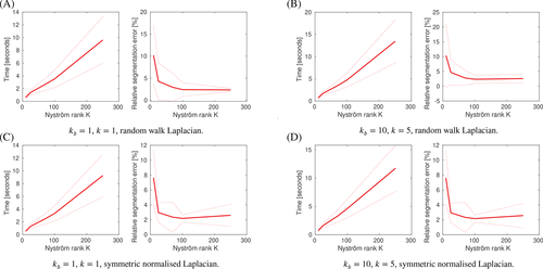
We now quantify the influence, on the accuracy and computational cost of the segmentation, of the Nyström rank K, the number of discretization steps kb and k in the Euler method and the Strang formula respectively, and the choice of normalization of the graph Laplacian. To this end, we segment the two cows image using the following parameters: , , , and . We take K ∈ {10, 25, 70, 100, 250}, (kb, k) ∈ {(1, 1), (10, 5)}, and use the random walk Laplacian and the symmetric normalized Laplacian .
We plot total runtimes (ie, the time elapsed from the loading of the image to be segmented, the reference data image, and the reference, to the output of the segmentation) and relative segmentation errors in Figure 13. As our method has randomness from the Nyström extension, we repeat every experiment 100 times and show means and standard deviations. We make several observations. Starting with the runtimes, we indeed see that these are roughly linear in K, verifying numerically the expected complexity. The runtime also increases when increasing kb and k. That is, increasing the accuracy of the Euler method and Strang formula does not lead to faster convergence, and also does not increase the accuracy of the overall segmentation. Finally, we see that the symmetric normalized Laplacian incurs consistently low relative segmentation error for small values of K. This property is of the utmost importance to scale up our algorithm for very large images. Interestingly, the segmentations using the symmetric normalized Laplacian seem to deteriorate for a large K. The random walk Laplacian has diametric properties in this regard: the segmentations are only reliably accurate when K is reasonably large.
4.3.2 Uncertainty in the segmentation
Due to the randomized Nyström approximation, our approximation of the SDIE scheme is inherently stochastic. Therefore, the segmentations that the algorithm returns are realizations of random variables. We now briefly study these random variables, especially with regard to K. We show pointwise mean and standard deviations of the binary labels in each of the left two columns of the four subfigures of Figure 14. In the remaining figures, we weight the original two cows image with these means (varying continuously between label 1 for “cow” and label 0 for “not cow”) and standard deviations. For these experiments we use the same parameter set-up as Section 4.3.1.
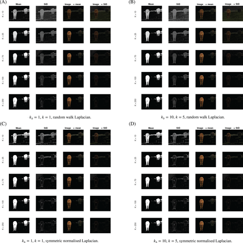
We make several observations. First, as K increases we see less variation. This is what we expect, as when K = |V| the method is deterministic so has no variation. Second, the type of normalization of the Laplacian has an effect: the symmetric normalized Laplacian leads to less variation than the random walk Laplacian. Third, the parameters kb and k appear to have no major effect within the range tested. Finally, looking at the figures with rather large K, we observe that the standard deviation of the labels is high in the areas of the figure in which there is indeed uncertainty in the segmentation, namely the boundaries of the cows and the parts of the wall with similar color to the dark cow. Determining the exact position of the boundary of a cow on a pixel-by-pixel level is indeed also difficult for a human observer. Moreover, the SDIE scheme usually confuses the wall in the background for a cow. Hence, a large standard deviation here reflects that the estimate is uncertain.
This is of course not a rigorous Bayesian uncertainty quantification, as for instance is given in 7, 37 for graph-based learning. However the use of stochastic algorithms for inference tasks, and the use of their output as a method of uncertainty quantification, has for instance been motivated by 31.
4.4 Grayscale
We now move on to Example 4.2, the grayscale problem. We will especially use this example to study the influence of the parameters and . The parameter determines the strength of the fidelity term in the ACE. From a statistical point of view, we can understand a choice of as an assumption on the statistical precision (ie, the inverse of the variance of the noise) of the reference (see [7, Section 3.3] for details). Thus, a small should lead to a stronger regularization coming from the Ginzburg-Landau functional, and a large leads to more adherence to the reference. The parameter is the “standard deviation” in the Gaussian kernel used to build the weight matrix . For our methods we must not choose too small a , as otherwise the weight matrix becomes sparse (up to some precision), and so the Nyström submatrix has a high probability of being ill-conditioned. In such a case this sparsity can be exploited using Rayleigh-Chebyshev 2 methods as in 32, or Matlab sparse matrix algorithms as in 6, but this lies beyond the scope of this paper. If is too large then the graph structure no longer reflects the features of the image.

In the following, we set , kb = 10, k = 5, and . To get reliable results we choose a rather large K, K = 200, and therefore (by the discussion in Section 4.3.2) we use the random walk Laplacian. We will qualitatively study single realizations of the inherently stochastic SDIE algorithm. We vary and . We show the best results from these tests in Figure 15. Moreover, we give a comprehensive overview of all tests and the progression of the SDIE scheme in Figure 16.
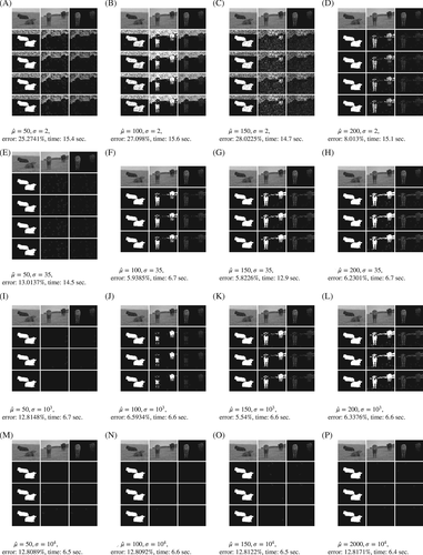
We observe that this segmentation problem is indeed considerably harder than the two cows problem, as we anticipated after stating Example 4.2. The difference in shade between the left cow and the wall is less visible than in Example 4.1, and the left cow's snout is less identifiable as part of the cow. Thus, the segmentation errors we incur are about three times larger than before. There is hardly any visible influence from changing in {35, 103}. However, and lead to significantly worse results. For , the sparsity (up to some precision) of the matrix deteriorates the results and the method becomes unstable; for , the weight matrix does not sufficient distinguish pixels of different shade, which is why the method labels everything as “not cow.”
Given in {35, 103}, the strength of the fidelity term has a significant impact on the result, as well. Indeed, for the algorithm does not find any segmentation. For , we get more practical segmentations. Interestingly, for and we get almost all of the left cow, but misclassify most of the wall in the background; for , we miss a large part of the left cow, but classify more accurately the wall. The interpretation of as the statistical precision of the reference explains this effect well. For , we assume that the reference is less precise, leading us (due to the smoothing effect of the Ginzburg-Landau regularization) to classify accurately most of the wall. With , we assume that the reference is more precise, leading us to misclassify the wall (due to its similarity to the cows in the reference data image) but classify accurately more of the cows. At , this effect even leads to a larger total segmentation error. The runtime varied throughout the experiments: the standard seems to be between 6 and 7 seconds. By doing an additional step in the iteration, the times for as well as are significantly increased. We also see a larger runtime in the case of .
4.5 Many cows
We finally study the many cows example, that is, Example 4.3. The main differences to the earlier examples are the larger size of the image that is to be segmented and the variety within it. We first comment on the size. The image is given by a 480 × 2560 × 3 tensor, which is a manageable size. The graph Laplacian, however, is a dense matrix with 1.536 × 10⁶ rows and columns. A matrix of this size requires 17.6 TB of memory to be constructed in MatlabR2019a. This image is much more difficult to segment than the previous examples, in which the cows in the image to be segmented are very similar to the cows in the reference data. Here, we have concatenated images of cows that look very different, for example, cows with a white blaze on their nose.
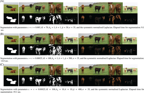
As the two cows image is part of the many cows image, we first test the algorithmic set-up that was successful at segmenting the former. We show the result (and remind the reader of the set-up) in Figure 17(a). The segmentation obtained in this experiment is rather mediocre—even the two cows part is only coarsely reconstructed. We present two more attempts at segmenting the many cows image in Figure 17: we choose , a slightly larger Nyström rank K = 100, and vary . In both cases, we obtain a considerably better segmentation of the image. In the case where , we see a good, but slightly noisy segmentation of the brown and black parts of the cows. In the case where , we reduce the noise in the segmentation, but then also misclassify some parts of the cows. The blaze (and surrounding fur) is not recognized as “cow” in any of the segmentations, likely because the blaze is not represented in the reference data image. The influence of the set-up on the runtimes is now much more pronounced. For the given segmentations, however, all the runtimes are at most a factor of eight larger than the smallest runtimes in the previous examples, despite the larger image size.
5 CONCLUSION
Extending the set-up and results in 13, we defined the continuous-in-time graph ACE with fidelity forcing as in 6 and a SDIE time discretization scheme for this equation. We proved well-posedness of the ACE and showed that solutions of the SDIE scheme converge to the solution of the ACE. Moreover, we proved that the graph MBO scheme with fidelity forcing 32 is a special case of an SDIE scheme.
We provided an algorithm to solve the SDIE scheme, which—besides the obvious extension from the MBO scheme to the SDIE scheme—differs in two key places from the existing algorithm for graph MBO with fidelity forcing: it implements the Nyström extension via a QR decomposition and it replaces the Euler discretization of the diffusion step with a computation based on the Strang formula for matrix exponentials. The former of these changes appears to have been a quite significant improvement: in experiments the Nyström-QR method proved to be faster, more accurate, and more stable than the Nyström method used in previous literature 6, 32, and it is less conceptually troubling than that method, as it does not involve taking the square root of a non-positive-semi-definite matrix.
- We found that the symmetric normalized Laplacian incurred consistently low segmentation error when approximated to a low rank, while the random walk Laplacian was more reliably accurate at higher ranks (where “higher” is still less than 0.1% of the full rank). Thus for applications that require scalability, and thus very low-rank approximations, we recommend using the symmetric normalized Laplacian.
- We investigated empirically the uncertainty inherited from the randomization in the Nyström extension. We found that the rank reduction and the normalization of the graph Laplacian had the most influence on the uncertainty, and we furthermore observed that at higher ranks the segmentations had high variance at those pixels which are genuinely difficult to classify, for example, the boundaries of the cows.
- We noted that the fidelity parameter corresponds to ascribing a statistical precision to the reference data. We observed that when the reference data were not fully informative, as in Examples 4.2 and 4.3, it was important to tune this parameter to get an accurate segmentation.
To conclude, we give a number of directions we hope to explore in future work, in no particular order.
We seek to investigate the use of the very recent method of 5 combined with methods such as the HMT method 26 or the (even more recent) generalized Nyström method 35 to further increase the accuracy of the low-rank approximations to the graph Laplacian. Unfortunately, we became aware of these works too near to finalizing this paper to use those methods here.
We will seek to extend both our theoretical and numerical framework to multiclass graph-based classification, as considered for example in 22, 28, 37. The groundwork for this extension was laid by the authors in [14, Section 6].
This work dovetails with currently ongoing work of the authors with Carola-Bibiane Schönlieb and Simone Parisotto exploring graph-based joint reconstruction and segmentation with the SDIE scheme. In practice, we often do not observe images directly, but must reconstruct an image from what we observe. For example, when the image is noisy, blurred, has regions missing, or we observe only a transform of the image, such as the output of a CT or MRI scanner. “Joint reconstruction and segmentation” (see 1, 17) is the task of simultaneously reconstructing and segmenting an image, which can reduce computational time and improve the quality of both the reconstruction and the segmentation.
We will also seek to develop an SDIE classification algorithm that is scalable towards larger data sets containing not just one, but hundreds or thousands of reference data images. This can be attempted via data subsampling: rather than evolving the SDIE scheme with regard to the full reference data set, we use only a data subset that is randomly replaced by a different subset after some time interval has passed. Data subsampling is the fundamental principle of various algorithms used in machine learning, such as stochastic gradient descent 38. A subsampling strategy that is applicable in continuous-in-time algorithms has recently been proposed and analyzed by 30.
ACKNOWLEDGEMENTS
We thank Andrea Bertozzi, Arjuna Flenner, and Arieh Iserles for very helpful comments. This work dovetails with ongoing work of the authors joint with Carola-Bibiane Schönlieb and Simone Parisotto, whom we therefore also thank for many indirect contributions. The work of Jeremy Budd and Yves van Gennip was supported by the European Union's Horizon 2020 research and innovation program under Marie Skłodowska-Curie grant 777826. The work of the Jonas Latz was supported by the EPSRC grant EP/S026045/1.
Appendix A: An analysis of the method from 32
Note.In fact, in 32 the authors use not . It makes no difference to this analysis which Laplacian is used.
A.1 Analysis
A.2 Conclusions from analysis
The key takeaway from these calculations (besides the verification that we have the usual Euler error) concerns (A6). That equation shows that the Euler approximation for the term is in fact an approximation of a Lie product formula approximation for . This motivates our method of cutting out the middleman and using a matrix exponential formula directly, and furthermore motivates our replacement of the linear error Lie product formula with the quadratic error Strang formula.
We have also shown how the Euler method approximation for b can be written as a form of quadrature, motivating our investigation of other quadrature methods as potential improvements for computing b.
References
- 1 for s > 0.
- 2 For the MBO case the thresholding is discontinuous so we do not get an analogous property.
- 3 .
- 4 More precisely, we will say for real (matrix) valued g, if and only if as in with the subspace topology induced by the standard topology on .
- 5 Suppose . Then .
- 6 Suppose . Then there exists U which is open in the topology of pointwise convergence such that x ∈ U and infinitely many xn ∉ U. Choose such that for all k, . This subsequence has no further subsubsequence converging to x.
- 7 It is easy to see that nonzero has negative eigenvalues, as it has zero trace.
- 8 The case of the random walk Laplacian is similar (due to the similarity of the matrices) except for a small additional error incurred by the approximation of D.
- 9 The HMT results serve only to give an additional benchmark for the Nyström methods: HMT requires matrix-vector-products with , which was infeasible for us in applications. However, as we were finalizing this paper we were made aware of the recent work of 5, which may make computing the HMT-SVD of feasible.
- 10 We owe the suggestion to use this formula to Arieh Iserles, who also suggested to us the Yoshida method that we consider below.
- 11 We again thank Arieh Iserles for also making this suggestion.
- 12 We can afford to do this for b, but not generally for the , because b only needs to be computed once rather than at each n.
- 13 Specifically, is incurred by the spectrum truncation in the middle of the latter term.
- 14 This method can be extended to give higher-order formulae of any even order, but consideration of those formulae is beyond the scope of this paper.
- 15 Accessed 20 October 2020.


