
A Forward Monte Carlo Method for American Options Pricing
We are grateful for the helpful comments and suggestions from Bob Webb (Editor) and an anonymous referee.
Abstract
This study proposes a forward Monte Carlo method for the pricing of American options. The main advantage of this method is that it does not use backward induction as required by other methods. Instead, the proposed approach relies on a wise determination about whether a simulated stock price has entered the exercise region. The validity of the proposed method is supported by the mathematical proofs for the vanilla cases. With some adaption, it is shown that this forward method can be extended to price other American style options such as chooser and exchange options. This study demonstrates the effectiveness of the proposed approach using a series of numerical examples, revealing significant improvements in numerical efficiency and accuracy in contrast with the standard regression-based method of Longstaff and Schwartz (2001). © 2012 Wiley Periodicals, Inc. Jrl Fut Mark 33:369-395, 2013
INTRODUCTION
Due to the lack of analytic solutions to American options prices, researchers have developed a number of methods for these pricing problems. Broadie and Detemple (2004) provided an excellent review summarizing the existing methods for the pricing of American options. Roughly speaking, these approaches can be separated into two main categories: the analytical approximation and the numerical methods. The former is dated back to Barone-Adesi and Whaley's (1987) quadratic approximation, which is regarded as the most representative work of its kind. Many subsequent studies extended their work to consider more complicated options or models, such as the recent examples of Chang, Kang, Kim, and Kim (2007) and Guo, Hung, and So (2009). On the other hand, Monte Carlo simulation is considered to be the most powerful numerical techniques for the valuation of American options. Unlike other methods (e.g., finite difference), the Monte Carlo method has higher flexibility, wider applicability to various products, and is convergent to the true values. Moreover, it is also less sensitive to the problem dimension and therefore better suited to pricing problems involving multiple assets.
Using Monte Carlo methods for option pricing dates back to Boyle (1977) for European options. Earlier applications of the Monte Carlo to American option pricing include Tilley's (1993) bundling algorithm, Barraquant and Martineau's (1995) stratified state aggregation algorithm, Broadie and Glasserman's (1997) stochastic tree based algorithm, Longstaff and Schwartz's (2001) regression-based algorithm. Boyle, Broadie, and Glasserman (1997) and Areal, Rodrigues, and Armada (2008) provide a comprehensive review of these methods. The Longstaff and Schwartz's method (also known as the least squares method [LSM]) is perhaps the most popular and promising one of these methods. Many researchers have adopted, modified, and extended this method over the years, including Clément, Lamberton, and Protter (2002), Gamba (2003), Glasserman and Yu (2004), Stentoft (2004a,2004b), Areal et al. (2008), and Liu (2010). The main idea of LSM is to estimate the continuation value through a least square regression on future simulated stock prices. This method simulates stock prices forward in time, but performs regression-based estimations successively in a backward manner like in a binomial tree. The LSM also helps alleviate the “curse of dimensionality” faced by tree-based methods, and is therefore appropriate for the valuation of a wide range of American options.
Despite its flexibility in its applications and robustness in the choice of regression function, the LSM still has the fundamental drawback of Monte Carlo methods, including slow convergence and high computational cost. The simulation error of a Monte Carlo method is generally in an order  , where M is the number of simulated paths (see, e.g., Peter, David, Martin, & Yan, 2005). Moreover, due to its free boundary nature, the Monte Carlo method generally performs worse in American than in European options pricing problems. American option pricing requires backward induction to find the optimal early exercise boundary, and existing methods differ mainly in the way the boundary is determined. In the original LSM, as proposed by Longstaff and Schwartz (2001), the necessity of backward induction is a major cause of numerical inefficiency (space and time) in that all the simulated paths of stock prices need to be stored (incurring space cost) and will be used later in the backward least square regression (incurring time cost). Areal et al. (2008) provided an improved version of LSM, which does not require all paths to be stored. However, backward induction still causes a significant amount of computation meaning that more time is needed to achieve higher accuracy.
 (1)
(1) is the payoff function and
  is the collection of stopping times, including maturity time T.
To determine whether the stock price has entered the exercise region, the FM resorts to the specification of the early exercise boundary as proposed in Barone-Adesi and Whaley (1987) (BAW). This important work shows that the approximate version of the optimal exercise boundary (critical price) for an American call or put option satisfies a nonlinear equation involving its corresponding European price. Though the critical price can be obtained by solving this nonlinear equation within a few iterations, solving such a nonlinear equation repeatedly during the simulation process is impractical because it creates a large computational burden. Therefore, the proposed approach defines a pseudo-critical price that satisfies a similar but simpler form of the nonlinear equation, allowing for quick computation. A mathematical analysis shows that this pseudo-critical price provides the full information as the real critical price (in the sense of BAW). This makes it possible to determine whether a given stock price has hit the exercise boundary at a given time through an efficient calculation without sacrificing accuracy. The proposed forward Monte Carlo method is then based on the real time computation of this pseudo-critical price through the process of simulation.
Because the pseudo-critical price is based on BAW, the FM relies on the availability of the European option pricing formula. Because there are many other options whose European prices have closed-form formulas, this approach is extendable to the pricing of their American counterparts. In fact, this extension requires an adaption from the vanilla case to other cases in consideration. More specifically, when the FM is adapted to other options, the pseudo-critical price must provide as much information as the real critical price regarding the determination of early exercise. This study extends the FM to price two other options including American chooser and exchange options. The theoretical proofs confirm that the proposed FM is suitable for these options and provides an efficient method for their pricing.
This study demonstrates the effectiveness of the proposed forward Monte Carlo method through a series of numerical examples comparing the performance of the FM with the LSM. The FM outperforms the LSM in all of the options discussed in this study. The FM generally achieves better accuracy (reducing the error of LSM by 12–50%) while solving the problem in only half of the time required by the LSM. One notable feature of the FM is that its accuracy does not deteriorate for options with longer maturities, which is not normally seen in other Monte Carlo methods using backward induction.
The rest of this study is organized as follows. In the next section, we present the central idea of the proposed FM and provide the theoretical justification for the vanilla cases. In the following section, we introduce how the FM can be extended to price other American options. In the section of numerical results, we give a number of examples to validate the proposed methods and quantify its improvement over the LSM. In the last section, we provide a conclusion.
THE FORWARD MONTE CARLO METHOD

Pseudo-Critical Prices
 for the call option should solve the nonlinear equation at any time
 (2)
(2) is the European call option price calculated by the Black–Scholes (1973) formula, K is the strike price, together with the notation
 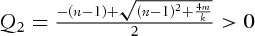 in which
  ,
,  , and
, and  . Note that this study uses more streamlined notations such as
  ,
,  when some dependent parameters are not stressed.
 on the right-hand side of (2) with the current stock price S yields a new but closely related function
 (3)
(3) represents the pseudo-critical price. The difference between
  and
and  is that solving (2) for
  requires an iterative procedure, while solving 3 for
  is only a function valuation. Note that the valuation of 3 requires the European price
  and the delta
  . When the stock price hits the critical price (
 ), then

Given the current price S, whether it is optimal to exercise the call early can be determined by  . Namely, the call should be held if
  and it should be exercised if
  . Note that the exact value of
  is not important. What is important here is whether it is possible to determine which one of
  and
and  is true. The following mathematical results show that under some conditions the critical price
  can provide as much information as the real critical price
  regarding the determination of early exercise.
Theorem 1.For an American call option with underlying stock price S and optimal early exercise price  , if the price of its European counterpart satisfies
  ,
,  (where
  is the gamma of a European call option) for all S, then

Proof 1.Define the following function:

 according to (2). We claim that
  is a strictly increasing function of S. To this end, first we show that
  . Suppose the opposite
  holds, that is,

 ,
,  ,
,  into the term above gives

 , we see immediate contradiction. Thus, assume
  . Squaring both sides with some calculations leads to

 and
and  . Thus, we have
  by contradiction. Therefore,

 ,
,  , and
, and  show that
  , indicating that
  is a strictly increasing function for all S. Consequently,

 iff
iff  is also true by the same argument, thus completing the proof.
Theorem 1 gives a theoretical justification of the usefulness of the pseudo-critical price  . For any given current price S, it is possible to calculate
  with much less cost and compare S with
  to determine if the option should be exercised. This property is the foundation on which the forward Monte Carlo method is based.
 must satisfy the following nonlinear equation:
 (4)
(4) . Replacing
  on the right-hand side of (4) with S, the pseudo-critical price
  is defined through the function
  as follows:
 (5)
(5) and the delta
  . Note that when
  , we must have
  . Like Theorem 1, Theorem 2 provides the conditions for the pseudo-critical price
  to be as informative as
  with regard to the determination of early exercise.
Theorem 2.Consider an American put option with an underlying stock price S and optimal early exercise price  . If the price of its European counterpart satisfies
  ,
,  (where
  is the gamma of a European put option) for all S, then

Proof 2.Define the following function:

 by (4). As in the previous proof, the objective is to claim
  is a strictly increasing function of S. Taking the derivative to see


 , the conditions
  ,
,  lead to
  and
and

 and therefore
  , again indicating
  is a strictly increasing function of S. Consequently,

 iff
iff  also holds, thus completing the proof.
Using these two main theorems as a foundation, in the following subsection, we present the proposed forward Monte Carlo method.
The FM for the American Vanilla Options
The notion of  and
and  carry the same information as
  and
and  can be made formal by the following definition.
Definition 1: The pseudo-critical price  is a sufficient indicator if it has the properties for all S: (1)
  if and only if
  , and (2)
  if and only if
  .
.
From the above definition, Theorems 1 and 2 give the sufficient conditions to check whether the pseudo-critical prices are actually sufficient indicators. Checking the Greeks of the vanilla options yields the following results.
Proposition 1.For both American vanilla call and put options, the pseudo-critical prices  and
and  defined in 3 and 5 are sufficient indicators.
Proof 3.The well-known formulas for the delta and gamma of European call and put options, that is,

 ,
,  ,
,  ,
,  . The claim follows from Theorems 1 and 2.
According to Proposition 1, using  and
and  to determine whether or not to exercise early is exactly the same as using
  and
and  . As calculating the former is much less computationally expensive than calculating the latter, the following forward Monte Carlo algorithm is then proposed to improve computational efficiency.
The forward Monte Carlo algorithm
- Generate M paths of stock prices, where each path
 evolves in discrete time with index
  (time interval
  ) as follows:

- If a given path i is alive (option not yet exercised) at time index
 , generate the price for time index j, denoted as
  .
.
-
In case of call option:
If
 , the option is expired with value
  and path i is finished.
If
 , calculate
  .
. If
 , the option is exercised with value
  and path i is stopped. Otherwise, the option is held and path continues to live to the next step
  .
. -
In case of put option:
If
 , the option is expired with value
  and path i is finished.
If
 , calculate
  .
. If
 , the option is exercised with value
  and path i is stopped. Otherwise, the option is held and path i continues to live to the next step
  .
.
-
- When all the simulation paths are completed, the American option is valued by averaging the discounted payoff as
Because the algorithm above uses no backward induction, it requires much less time and space than other Monte Carlo methods. Note that the method affords significant space savings because it does not need to store all simulated paths. Each time the stock price moves one step forward, the past stock price is no longer needed and can be discarded. On the other hand, backward induction based methods (e.g., the binomial tree method, and the original LSM, and other Monte Carlo methods) usually need to store some, if not all, of the path information to determine critical prices in the backward process. Boyle et al. (1997) noted that, Tilley's (1993) algorithm requires all paths to be stored, yielding a storage cost in an order of  , where M and N are the numbers of paths and time steps. Barraquant and Martineau's (1995) algorithm improves storage efficiency and reduces the order to
  , where k is the number of disjoint cells. The standard LSM presented by Longstaff and Schwartz (2001) has a typical order of storage cost
  . The proposed FM only requires a minimal order O(1) of storage (if only the necessary results are stored), and outperforms other methods greatly.1
EXTENSIONS TO OTHER AMERICAN OPTIONS
In addition to vanilla options, the proposed FM can be extended to price a number of other American options for which the analytic pricing formulas of their European counterparts are available. This extension requires an examination of whether the corresponding pseudo-critical price can be defined and the desired property remains. The proposed algorithm is adapted to fit each specific type of option. In this section, we discuss how the proposed method can be extended to two types of options: American chooser and exchange options.
American Chooser Options
 . For
. For  , the option type is determined and both the European and American options are treated as if they are vanilla call or put options. At
  , the European and American chooser options prices are the maximum of the corresponding call and put prices, that is,

 , the price of European chooser option is given by (see Rubinstein, 1991)
 (6)
(6) and
and  are given by

 with the proposed FM.
Because the American chooser option can be exercised as either a call or a put when  , its exercise value is
  . The strike price K is a natural boundary for determining the option type it tends to be, that is, it can be viewed as an American call if
  or put if
  . Early exercise is optimal when S is sufficiently large (exercised as a call) or small (exercised as a put). In other words, there is a pair of upper and lower critical prices
  and
and  . The American chooser option remains alive if
  , and will be exercised either
  or
or  .
.
 and
and  , which are defined in a similar way to 3 and 5 as
 (7)
(7) (8)
(8) should be an increasing function of S like the vanilla call price
  for
for  , and not too close to K. Likewise, it should be a decreasing function of S like the vanilla put price
  for
for  and not too close to K. In other words,
  should carry the same mathematical properties of vanilla call or put prices when the option tends to be a call or put, respectively.
The validity of the proposed FM depends on whether  and
and  can determine if the stock price has entered the exercise regions. Namely, it remains to ask whether they are sufficient indicators as defined in Definition 1. The following proposition shows that this is indeed the case.
Proposition 2.For an American chooser option at  , the upper and lower pseudo-critical prices
  and
and  are sufficient indicators in the sense that

 ,
,  , and
, and

 ,
,  .
.
Proof 4.From 6, the delta and gamma of European chooser option is given by

 if
if  and vice versa, but
  is always true. Consequently, when it tends to be a call with
  and
and  ,
,  is a sufficient indicator according to Theorem 1. Similarly, when it tends to be a put with
  and
and  ,
,  is also a sufficient indicator according to Theorem 2.
Consequently, the decision of whether it should be exercised early can be made by comparing the current stock price S with both the pseudo-critical prices  or
or  . The difference between the chooser and vanilla cases is its dual nature, but this does not mean that both
  and
and  must be calculated at each time step through the simulation. Note that the algorithm will determine the tendency of a call or put along with the simulated paths by checking
  ,
,  or
or  ,
,  . Depending on the type tendency, it is only necessary to use either
  or
or  to make the early exercise decision. Although neither is true, the stock price should be around the strike price, that is,
  and
and  . In other words, the option is close to at-the-money, and is neither large or small enough for the early exercise to be an optimal decision.
- When
 :
:
-
If
 ,
,  :
:
If
 , the option is exercised as a call.
Otherwise it will be held until the next time step.
-
If
 ,
,  :
:
If
 , the option is exercised as a put.
Otherwise it will be held until the next time step.
-
Neither (i) nor (ii) is true:
The option is held until the next time step.
-
-
When
 :
:If
 , the option is chosen to be a call. Otherwise, it is chosen to be a put.2
 -
When
 :
:The simulation progresses as if it is an American vanilla option.
American Exchange Options
 follow
  ,
,  , and
, and  . Namely,
  ,
,  denote the dividend yield and volatility of
  , and ρ represents their correlation. For the European exchange option, which provides a T-payoff
  , its t-price is given in closed form by


 is the volatility of the process
  whose dynamics can be described as below:

 , and its t-price has the following alternative form:


 , or when
  is sufficiently large. In fact, if S2 is taken to be a numeraire, this problem can be viewed as an American vanilla option pricing problem in terms of Y such as the above European case. This point is discussed in Gounden and O'Hara (2009) (Theorem 4.1), Bjerksund and Stensland (1993), and Choi and Ahn (2002), and can be expressed as the following simple relation:

 is large enough to trigger early exercise, then the process Y must hit the critical price
  at the same time τ. Therefore, to determine the early exercise of the original exchange option, one may simply look at the process Y and determine whether early exercise is optimal by checking if it has crossed the critical price
  .
. (9)
(9)Proposition 3.For American exchange options, the pseudo-critical price  as in 9 is a sufficient indicator in the sense that

Proof 5.The claim can be proven by showing that the delta and gamma for the call option on  satisfy the conditions in Theorem 1.

The algorithm adaption follows directly from Proposition 3. In the simulation of the paths of the two stock prices, at each time step, it is necessary to calculate  and compare it with
  . Once the exercise condition is triggered, that is,
  , the value of
  is exercised. The American exchange option is then obtained by averaging the discounted values of all simulated paths.3
NUMERICAL RESULTS
In this section, we present numerical results to demonstrate the effectiveness of the proposed FM. The options considered here are those discussed in the preceding sections, including American vanilla call and put options, chooser options, and exchange options. The numerical study examines the accuracy and computation efficiency of the FM and compares it with the LSM and the benchmark values obtained from the binomial method. Moreover, this study also looks at the convergence of the proposed method as both the number of time steps and simulated paths increase.
In the implementation of the LSM, we follow the suggestion of Longstaff and Schwartz (2001) and use only in-the-money paths in the regression to estimate the continuation value. This will help improve the computational efficiency and accuracy. Moreover, Areal et al. (2008) also reported that, compared with a standard regression algorithm, using the least-squares FIT algorithm may speed up the regression by one-third. In the interest of comparing our FM with the LSM that is known to be more efficient, the LFIT algorithm is used for the regression in our numerical study.

 is the true (benchmark) American option value for the ith parameter set,
  is the corresponding estimate from simulation, and G is the number of parameter sets in a given group. Computational efficiency is measured through CPU time (seconds), and all numerical experiments are carried out in MATLAB on a PC with the following specification: Intel Pentium(R) Dual-Core CPU E6500 2.93 GHz and 4-GB RAM.
American Vanilla Options
The numerical analysis begins with the American vanilla call and put options. To compare the FM with the LSM, this study uses the same parameter sets as in Longstaff and Schwartz (2001),4 where the initial stock price  36, 38, 40, 42, and 44, time to expiration
  1, 2, volatility
  0.2, 0.4. The other parameters remain fixed, including strike price
  40, risk-free interest rate
  0.04, and dividend yield
  0.06. In Tables I and II we present the results, comparing both the LSM and FM5, 6 against the binomial method results obtained from the CRR tree with 10,000 time steps. The results from both simulation methods are based on 100,000 paths. According to Longstaff and Schwartz (2001), three basis functions are sufficient to obtain effective convergence for an American vanilla option. Therefore, in these examples of vanilla options, the LSM uses polynomial basis functions up to the third power, that is,
  .
.
| Parameters | Binomial Tree | LSM | Forward Method | |||||||||
|---|---|---|---|---|---|---|---|---|---|---|---|---|
| S | T | σ | Price | Time | Price | RE (%) | (SE) | Time | Price | RE (%) | (SE) | Time |
| 36 | 1 | 0.2 | 1.1953 | 11.5 | 1.1891 | −0.52 | (0.008) | 1.0 | 1.2002 | 0.41 | (0.008) | 0.6 |
| 38 | 1 | 0.2 | 1.8793 | 11.6 | 1.8752 | −0.22 | (0.010) | 1.2 | 1.8693 | −0.53 | (0.010) | 0.7 |
| 40 | 1 | 0.2 | 2.7688 | 11.6 | 2.7676 | −0.04 | (0.012) | 1.5 | 2.7777 | 0.32 | (0.012) | 0.8 |
| 42 | 1 | 0.2 | 3.8658 | 11.6 | 3.8710 | 0.13 | (0.013) | 1.7 | 3.8735 | 0.20 | (0.014) | 0.9 |
| 44 | 1 | 0.2 | 5.1616 | 11.6 | 5.1645 | 0.06 | (0.014) | 1.9 | 5.1736 | 0.23 | (0.015) | 0.9 |
| 36 | 1 | 0.4 | 3.8192 | 11.6 | 3.7994 | −0.52 | (0.022) | 1.2 | 3.8014 | −0.47 | (0.023) | 0.7 |
| 38 | 1 | 0.4 | 4.7537 | 11.6 | 4.7334 | −0.43 | (0.024) | 1.3 | 4.7487 | −0.10 | (0.026) | 0.7 |
| 40 | 1 | 0.4 | 5.7926 | 11.6 | 5.7805 | −0.21 | (0.027) | 1.4 | 5.7967 | 0.07 | (0.028) | 0.8 |
| 42 | 1 | 0.4 | 6.9313 | 11.6 | 6.9286 | −0.04 | (0.029) | 1.5 | 6.9312 | 0.00 | (0.030) | 0.9 |
| 44 | 1 | 0.4 | 8.1635 | 11.6 | 8.1669 | 0.04 | (0.031) | 1.7 | 8.1554 | −0.10 | (0.033) | 0.9 |
| 36 | 2 | 0.2 | 1.9831 | 11.5 | 1.9699 | −0.67 | (0.012) | 2.2 | 1.9740 | −0.46 | (0.012) | 1.2 |
| 38 | 2 | 0.2 | 2.7389 | 11.6 | 2.7212 | −0.65 | (0.014) | 2.5 | 2.7351 | −0.14 | (0.014) | 1.3 |
| 40 | 2 | 0.2 | 3.6467 | 11.6 | 3.6358 | −0.30 | (0.015) | 2.9 | 3.6487 | 0.06 | (0.016) | 1.5 |
| 42 | 2 | 0.2 | 4.7070 | 11.6 | 4.7094 | 0.05 | (0.017) | 3.2 | 4.6965 | −0.22 | (0.018) | 1.6 |
| 44 | 2 | 0.2 | 5.9167 | 11.6 | 5.9287 | 0.20 | (0.018) | 3.5 | 5.9157 | −0.02 | (0.019) | 1.6 |
| 36 | 2 | 0.4 | 5.6516 | 11.6 | 5.6032 | −0.86 | (0.032) | 2.5 | 5.6305 | −0.37 | (0.033) | 1.4 |
| 38 | 2 | 0.4 | 6.6506 | 11.6 | 6.5937 | −0.86 | (0.035) | 2.7 | 6.6662 | 0.23 | (0.036) | 1.4 |
| 40 | 2 | 0.4 | 7.7238 | 11.6 | 7.6479 | −0.98 | (0.036) | 2.9 | 7.7271 | 0.04 | (0.039) | 1.5 |
| 42 | 2 | 0.4 | 8.8684 | 11.6 | 8.8221 | −0.52 | (0.039) | 3.0 | 8.8624 | −0.07 | (0.041) | 1.6 |
| 44 | 2 | 0.4 | 10.0799 | 11.6 | 10.0530 | −0.27 | (0.041) | 3.1 | 10.1127 | 0.33 | (0.043) | 1.7 |
| Average | RMSE = 0.48% | 2.1 | RMSE = 0.27% | 1.1 | ||||||||
Note
- Option parameters other than the stock price S, maturity T, and volatility σ as shown above include the strike price
 , interest rate
  , and dividend yield
  . Simulation results are based on 100,000 paths. The values in parentheses are the standard errors (SE) of the simulation estimates from both methods.
| Parameters | Binomial Tree | LSM | Forward Method | |||||||||
|---|---|---|---|---|---|---|---|---|---|---|---|---|
| S | T | σ | Price | Time | Price | RE (%) | (SE) | Time | Price | RE (%) | (SE) | Time |
| 36 | 1 | 0.2 | 4.4779 | 11.5 | 4.4740 | −0.09 | (0.009) | 1.8 | 4.4784 | 0.01 | (0.010) | 0.6 |
| 38 | 1 | 0.2 | 3.2502 | 11.6 | 3.2482 | −0.06 | (0.009) | 1.7 | 3.2555 | 0.16 | (0.010) | 0.7 |
| 40 | 1 | 0.2 | 2.3141 | 11.6 | 2.3084 | −0.24 | (0.009) | 1.4 | 2.3017 | −0.53 | (0.009) | 0.7 |
| 42 | 1 | 0.2 | 1.6170 | 11.6 | 1.6145 | −0.16 | (0.008) | 1.2 | 1.6171 | 0.00 | (0.008) | 0.6 |
| 44 | 1 | 0.2 | 1.1099 | 11.6 | 1.1130 | 0.28 | (0.007) | 1.1 | 1.1132 | 0.30 | (0.007) | 0.6 |
| 36 | 1 | 0.4 | 7.1013 | 19.0 | 7.0953 | −0.08 | (0.019) | 1.8 | 7.1074 | 0.09 | (0.019) | 0.8 |
| 38 | 1 | 0.4 | 6.1477 | 19.0 | 6.1338 | −0.23 | (0.018) | 1.6 | 6.1418 | −0.10 | (0.019) | 0.8 |
| 40 | 1 | 0.4 | 5.3119 | 19.1 | 5.3018 | −0.19 | (0.018) | 1.5 | 5.3097 | −0.04 | (0.018) | 0.8 |
| 42 | 1 | 0.4 | 4.5825 | 19.1 | 4.5693 | −0.29 | (0.017) | 1.4 | 4.5624 | −0.44 | (0.017) | 0.7 |
| 44 | 1 | 0.4 | 3.9477 | 19.1 | 3.9450 | −0.07 | (0.016) | 1.3 | 3.9364 | −0.29 | (0.017) | 0.7 |
| 36 | 2 | 0.2 | 4.8403 | 11.5 | 4.8362 | −0.08 | (0.011) | 3.4 | 4.8347 | −0.12 | (0.011) | 1.1 |
| 38 | 2 | 0.2 | 3.7448 | 11.6 | 3.7344 | −0.28 | (0.011) | 3.1 | 3.7398 | −0.13 | (0.011) | 1.2 |
| 40 | 2 | 0.2 | 2.8846 | 11.6 | 2.8676 | −0.59 | (0.010) | 2.9 | 2.8944 | 0.34 | (0.011) | 1.2 |
| 42 | 2 | 0.2 | 2.2124 | 11.6 | 2.2072 | −0.24 | (0.010) | 2.5 | 2.2119 | −0.03 | (0.010) | 1.2 |
| 44 | 2 | 0.2 | 1.6899 | 11.6 | 1.6908 | 0.06 | (0.009) | 2.3 | 1.6869 | −0.18 | (0.009) | 1.1 |
| 36 | 2 | 0.4 | 8.5069 | 19.0 | 8.4722 | −0.41 | (0.022) | 3.4 | 8.5019 | −0.06 | (0.023) | 1.5 |
| 38 | 2 | 0.4 | 7.6682 | 19.0 | 7.6480 | −0.26 | (0.022) | 3.2 | 7.6725 | 0.06 | (0.022) | 1.5 |
| 40 | 2 | 0.4 | 6.9170 | 19.0 | 6.8969 | −0.29 | (0.022) | 3.0 | 6.9168 | 0.00 | (0.022) | 1.4 |
| 42 | 2 | 0.4 | 6.2445 | 19.1 | 6.2331 | −0.18 | (0.021) | 2.9 | 6.2262 | −0.29 | (0.021) | 1.4 |
| 44 | 2 | 0.4 | 5.6414 | 19.1 | 5.6242 | −0.31 | (0.021) | 2.7 | 5.6491 | 0.14 | (0.021) | 1.3 |
| Average | RMSE = 0.25% | 2.2 | RMSE = 0.22% | 1.0 | ||||||||
 , interest rate
  , and dividend yield
  . The simulation is based on 100,000 paths.
In Table I we show the results of vanilla calls, indicating that the FM apparently outperforms the LSM in terms of both accuracy and computing time. The FM achieves a better RMSE (56% of LSM) with nearly a half of computing time (52% of LSM). This significant reduction in computing time is certainly because no backward induction is required, and forward evolution may stop early at some optimal exercise point. The slightly improved RMSE indicates that the pseudo-critical prices work well, and determine the exercise time correctly. Similar observations can be made for the vanilla puts in Table II. Once again, the FM requires much less computing time (45% of LSM) to achieve an improvement in RMSE (88% of LSM).
Note that the FM relies on a quadratic approximation of BAW, which is not an exact result. BAW (1987) claimed that the approximation of both the American option price and the critical price will slightly deteriorate as the time to expiration becomes longer (e.g., beyond one year). It is therefore interesting to examine whether a long time-to-maturity influences the FM performance. For this purpose, the accuracy of the original data set in the BAW (1987) paper (p. 317, Table V) is compared with the accuracy of the FM. In Table III, we present these results indicating that the FM still performs well when the time-to-maturity is  . The accuracy of the FM for both call and put options remains at a level comparable to Tables I and II (with RE normally less than 0.8% with RMSE = 0.28%). The accuracy of the LSM is also comparable to Tables I and II but seems to be slightly worse (with RMSE = 0.56%) when pricing options with long time-to-maturity. However, the error in the original quadratic approximation of BAW (1987) becomes relatively larger than the short time-to-maturity case with
  (RE ranged roughly in 1–7% with RMSE = 3.15%).
| Parameters | BAW | LSM | Forward Method | |||||||||
|---|---|---|---|---|---|---|---|---|---|---|---|---|
 |
S | Binomial Price | Price | RE (%) | Price | RE (%) | (SE) | Time | Price | RE (%) | (SE) | Time |
| Call | ||||||||||||
 |
80 | 2.3415 | 2.5238 | 7.78 | 2.3162 | −0.91 | (0.021) | 2.7 | 2.3298 | −0.50 | (0.020) | 1.5 |
 |
90 | 4.7591 | 4.9664 | 4.36 | 4.6820 | −1.47 | (0.028) | 3.3 | 4.7724 | 0.28 | (0.029) | 1.6 |
 |
100 | 8.4935 | 8.6696 | 2.07 | 8.4300 | −0.60 | (0.035) | 4.1 | 8.5034 | 0.12 | (0.036) | 1.8 |
 |
110 | 13.7937 | 13.8817 | 0.64 | 13.7721 | −0.02 | (0.040) | 4.8 | 13.7240 | −0.51 | (0.042) | 1.7 |
 |
120 | 20.8889 | 20.8816 | −0.03 | 20.8547 | −0.03 | (0.038) | 5.3 | 20.8400 | −0.23 | (0.040) | 1.2 |
 |
80 | 3.9827 | 4.2026 | 5.52 | 3.9472 | −0.85 | (0.030) | 3.0 | 4.0068 | 0.60 | (0.030) | 1.7 |
 |
90 | 7.2506 | 7.5366 | 3.94 | 7.1879 | −0.82 | (0.039) | 3.6 | 7.2587 | 0.11 | (0.041) | 1.9 |
 |
100 | 11.7037 | 12.0302 | 2.79 | 11.6380 | −0.52 | (0.048) | 4.4 | 11.6176 | −0.74 | (0.050) | 2.3 |
 |
110 | 17.3156 | 17.6413 | 1.88 | 17.2784 | −0.17 | (0.055) | 5.2 | 17.3255 | 0.06 | (0.058) | 2.5 |
 |
120 | 24.0189 | 24.2966 | 1.16 | 24.0466 | 0.16 | (0.060) | 5.8 | 24.0536 | 0.14 | (0.063) | 2.3 |
 |
80 | 6.8820 | 6.9653 | 1.21 | 6.8020 | −1.16 | (0.045) | 3.3 | 6.8790 | −0.04 | (0.048) | 1.9 |
 |
90 | 11.4931 | 11.6209 | 1.11 | 11.3915 | −0.88 | (0.059) | 4.0 | 11.4969 | 0.03 | (0.063) | 2.4 |
 |
100 | 17.2145 | 17.3989 | 1.07 | 17.1476 | −0.39 | (0.075) | 4.7 | 17.1582 | −0.33 | (0.078) | 3.1 |
 |
110 | 23.8410 | 24.0919 | 1.05 | 23.7887 | −0.22 | (0.088) | 5.8 | 23.8219 | −0.08 | (0.092) | 3.9 |
 |
120 | 31.1656 | 31.4912 | 1.04 | 31.0677 | −0.31 | (0.097) | 6.2 | 31.2445 | 0.25 | (0.105) | 4.2 |
| Put | ||||||||||||
 |
80 | 25.6577 | 26.2452 | 2.29 | 25.6425 | −0.05 | (0.045) | 6.2 | 25.6352 | −0.09 | (0.048) | 3.4 |
 |
90 | 20.0832 | 20.6410 | 2.78 | 20.0351 | −0.23 | (0.046) | 6.0 | 20.0516 | −0.16 | (0.048) | 3.6 |
 |
100 | 15.4981 | 15.9902 | 3.18 | 15.4181 | −0.51 | (0.044) | 5.1 | 15.4697 | −0.18 | (0.046) | 3.1 |
 |
110 | 11.8032 | 12.2212 | 3.54 | 11.7390 | −0.54 | (0.041) | 4.3 | 11.7938 | −0.08 | (0.042) | 2.6 |
 |
120 | 8.8856 | 9.2345 | 3.93 | 8.8273 | −0.65 | (0.037) | 3.8 | 8.8752 | −0.12 | (0.038) | 2.3 |
 |
80 | 22.2050 | 22.3950 | 0.86 | 22.2028 | 0.03 | (0.036) | 6.0 | 22.1734 | −0.14 | (0.038) | 2.0 |
 |
90 | 16.2071 | 16.4976 | 1.79 | 16.1777 | −0.14 | (0.039) | 5.7 | 16.1904 | −0.10 | (0.040) | 2.4 |
 |
100 | 11.7037 | 12.0302 | 2.79 | 11.6609 | −0.32 | (0.037) | 4.7 | 11.6879 | −0.14 | (0.037) | 2.3 |
 |
110 | 8.3671 | 8.6871 | 3.82 | 8.3361 | −0.33 | (0.033) | 4.0 | 8.3595 | −0.09 | (0.034) | 2.0 |
 |
120 | 5.9299 | 6.2222 | 4.93 | 5.9015 | −0.44 | (0.029) | 3.5 | 5.9208 | −0.15 | (0.029) | 1.8 |
 |
80 | 20.3500 | 20.3255 | −0.12 | 20.3181 | −0.05 | (0.024) | 5.7 | 20.3051 | −0.22 | (0.026) | 0.9 |
 |
90 | 13.4968 | 13.5631 | 0.49 | 13.4411 | −0.30 | (0.032) | 5.2 | 13.4737 | −0.17 | (0.032) | 1.7 |
 |
100 | 8.9438 | 9.1076 | 1.83 | 8.8944 | −0.43 | (0.031) | 4.3 | 8.9304 | −0.15 | (0.031) | 1.8 |
 |
110 | 5.9119 | 6.1225 | 3.56 | 5.8895 | −0.25 | (0.027) | 3.7 | 5.8864 | −0.43 | (0.027) | 1.7 |
 |
120 | 3.8975 | 4.1153 | 5.59 | 3.8854 | −0.17 | (0.022) | 3.1 | 3.8884 | −0.23 | (0.022) | 1.6 |
| Average | RMSE = 3.15% | RMSE = 0.56% | 4.6 | RMSE = 0.28% | 2.2 | |||||||
Note
- The option parameters are given by the Table V (p. 317) in Barone-Adesi and Whaley (1987). The benchmark prices are obtained by the binomial method with 10,000 time steps (each time step is exercisable before the maturity time). For the forward method, the simulation is based on 100,000 paths. The main difference in parameters is the long time-to-maturity
 , with other parameters, stock price S, interest rate r, dividend yield q, volatility σ, strike price K, remained at typical levels.
The reason for this observation is that the quadratic approximation of BAW (1987) expresses the American option prices in terms of the critical prices  . When
  includes error due to a long time-to-maturity, it carries over to the American option prices. On the contrary, the FM algorithm is generally less sensitive to the accuracy of
  and
and  . Li (2010) compared the accuracy of critical prices from different approximation methods, showing that the error is reported to be about 2% for the
  in BAW (1987). However, the error would not go to the final option price in a proportional way because in the FM, the error in critical prices just means a few paths are not exercised at the optimal time, and the slight loss of optimality does not have strong effect. Ju and Zhong (1999) claimed that a very accurate estimate of the early exercise boundary is not required to price an American options accurately. This demonstrates the robustness of the FM in that it is suitable for the pricing problems when the time-to-maturity is long.
American Chooser Options
In the numerical example of American chooser options, the option parameters largely follow Table III, with the exception that it is necessary to specify the date of choice  separately from the maturity time
  . Among the 50 exercisable time steps during option's life, half of them are in the interval prior to
  . The implementation of the LSM employs these basis functions:
  , and their cross-product terms
  ,
,  ,
,  up to the third power (
 ).7 Therefore, there are a total of ten basis functions used in the regression. Because the dual nature of a chooser option makes it more complicated than vanilla options, one may expect it requires more basis functions to characterize the regression relation.
In Table IV, we compare the LSM and the FM against the binomial method, again revealing a nice improvement in both computing time and accuracy. The improvement in computing time is significant but not as good as what are seen in the previous vanilla cases. For chooser options, the FM takes two-thirds of the time taken by the LSM to carry out the option valuation, whereas it takes a half of time of the LSM for the valuation of vanilla options. The improvement in accuracy is also significant, with RMSE being 0.18% for the FM in contrast with 0.32% for the LSM.
| Parameters | Binomial Tree | LSM | Forward Method | ||||||||
|---|---|---|---|---|---|---|---|---|---|---|---|
 |
σ | Price | Time | Price | RE (%) | (SE) | Time | Price | RE (%) | (SE) | Time |
| 80 | 0.2 | 21.4097 | 11.2 | 21.3866 | −0.11 | (0.033) | 3.3 | 21.4208 | 0.05 | (0.036) | 2.1 |
| 90 | 0.2 | 15.2232 | 11.2 | 15.2123 | −0.07 | (0.033) | 3.3 | 15.2465 | 0.15 | (0.035) | 2.5 |
| 100 | 0.2 | 13.1881 | 11.2 | 13.1584 | −0.23 | (0.031) | 3.2 | 13.1660 | −0.17 | (0.034) | 2.5 |
| 110 | 0.2 | 15.7419 | 11.2 | 15.6796 | −0.40 | (0.033) | 3.2 | 15.7319 | −0.06 | (0.038) | 2.2 |
| 120 | 0.2 | 21.9060 | 11.2 | 21.9032 | −0.01 | (0.037) | 3.2 | 21.9172 | 0.05 | (0.041) | 1.7 |
| 80 | 0.4 | 28.8851 | 11.2 | 28.8362 | −0.17 | (0.054) | 3.3 | 28.9318 | 0.16 | (0.056) | 2.1 |
| 90 | 0.4 | 26.2775 | 11.2 | 26.2195 | −0.22 | (0.057) | 3.2 | 26.3799 | 0.39 | (0.060) | 2.2 |
| 100 | 0.4 | 26.2087 | 11.2 | 26.2116 | 0.01 | (0.068) | 3.2 | 26.2893 | 0.31 | (0.066) | 2.3 |
| 110 | 0.4 | 28.4653 | 11.2 | 28.2911 | −0.61 | (0.072) | 3.2 | 28.4585 | −0.02 | (0.073) | 2.2 |
| 120 | 0.4 | 32.6841 | 11.2 | 32.4846 | −0.61 | (0.078) | 3.2 | 32.6628 | −0.06 | (0.081) | 2.1 |
| Average | RMSE = 0.32% | 3.2 | RMSE = 0.18% | 2.2 | |||||||
Note
- Option parameters other than stock price S and volatility σ are as follows: strike price
 , interest rate
  , dividend yield
  , date of choice
  , and time-to-maturity
  . The simulation is based on 100,000 paths.
American Exchange Options
The final example is American exchange options involving two stock prices. The option parameters are similar to the preceding case of chooser options. Keeping the first stock price  fixed, this study varies the second stock price S2 among the values 80, 90, 100, 110, and 120, and considers three possible correlations between them:
  0.5, 0, and −0.5. Other parameters remain fixed, including the interest rate
  , dividend yields for both stocks
  ,
,  , and their volatilities
  ,
,  . The basis functions are chosen to be
  ,
,  ,
,  ,
,  up to the third power (
 ) and thus there are totally ten basis functions.8 A two-dimensional binomial tree based on the method of Boyle, Evnine, and Gibbs (1989) serves as a benchmark with 1,000 time steps.
In Table V we present the results, showing an improvement similar to the preceding examples, that is, the FM once again takes about a third of the time to achieve a better accuracy. Because an exchange option involves two assets, it is expected that more computing time is required, and the times consumed by both simulation methods are in proportion to the single asset examples, such as vanilla options in Tables I and II. The LSM error seems to remain at a level comparable to vanilla options (mostly less than 0.5% with RMSE = 0.25%), but is still larger than the FM (RMSE = 0.19%). Also note that for both methods, the errors tend to stay at the same level when correlation varies, indicating that they are both robust under different ρ. The errors across different cases of ρ appear to exhibit an irregular pattern, while the FM yields a smaller error in most cases.
| Parameters | Binomial Tree | LSM | Forward Method | ||||||||
|---|---|---|---|---|---|---|---|---|---|---|---|
 |
ρ | Price | Time | Price | RE (%) | (SE) | Time | Price | RE (%) | (SE) | Time |
| 80 | 0.5 | 23.3023 | 33.4 | 23.3294 | 0.12 | (0.052) | 5.2 | 23.3045 | 0.01 | (0.051) | 1.5 |
| 90 | 0.5 | 17.2995 | 33.4 | 17.3348 | 0.20 | (0.053) | 4.7 | 17.3425 | 0.25 | (0.052) | 1.7 |
| 100 | 0.5 | 12.6822 | 33.4 | 12.6855 | 0.03 | (0.049) | 4.1 | 12.6726 | −0.08 | (0.048) | 1.8 |
| 110 | 0.5 | 9.1659 | 33.4 | 9.1639 | −0.02 | (0.043) | 3.7 | 9.1769 | 0.12 | (0.043) | 1.7 |
| 120 | 0.5 | 6.5800 | 33.5 | 6.5944 | 0.22 | (0.038) | 3.2 | 6.5418 | −0.58 | (0.038) | 1.7 |
| 80 | 0 | 27.3141 | 33.4 | 27.2768 | −0.14 | (0.072) | 4.9 | 27.3597 | 0.17 | (0.073) | 1.7 |
| 90 | 0 | 22.1558 | 33.6 | 22.2306 | 0.34 | (0.073) | 4.6 | 22.1423 | −0.06 | (0.072) | 1.8 |
| 100 | 0 | 17.8982 | 33.4 | 17.9325 | 0.19 | (0.070) | 4.1 | 17.9143 | 0.09 | (0.069) | 1.8 |
| 110 | 0 | 14.4697 | 33.6 | 14.5380 | 0.47 | (0.065) | 3.8 | 14.4532 | −0.11 | (0.065) | 1.8 |
| 120 | 0 | 11.6713 | 33.6 | 11.7288 | 0.49 | (0.062) | 3.5 | 11.6940 | 0.19 | (0.061) | 1.8 |
| 80 | −0.5 | 30.6439 | 33.4 | 30.5995 | −0.14 | (0.086) | 4.9 | 30.6311 | −0.04 | (0.088) | 1.9 |
| 90 | −0.5 | 25.8842 | 33.4 | 25.8429 | −0.16 | (0.087) | 4.5 | 25.8733 | −0.04 | (0.087) | 1.9 |
| 100 | −0.5 | 21.9251 | 33.5 | 21.9504 | 0.12 | (0.085) | 4.2 | 21.9198 | −0.02 | (0.085) | 1.8 |
| 110 | −0.5 | 18.5688 | 33.5 | 18.5309 | −0.20 | (0.080) | 3.8 | 18.5485 | −0.11 | (0.082) | 1.8 |
| 120 | −0.5 | 15.7835 | 33.6 | 15.8334 | 0.32 | (0.077) | 3.6 | 15.7957 | 0.08 | (0.078) | 1.7 |
| Average | RMSE = 0.25% | 4.2 | RMSE = 0.19% | 1.8 | |||||||
Note
- The first stock price is fixed (
 ), whereas the second stock price takes one of the following values:
  80, 90, 100, 110, and 120. Three correlation coefficients are considered:
  0.5, 0, and −0.5. Other parameters include the interest rate
  , dividend yields
  ,
,  , volatilities
  ,
,  , and maturity
  . The simulation is based on 100,000 paths. The benchmark values are from a two-dimensional binomial tree based on the method of Boyle, Evnine, and Gibbs (1989) with 1,000 time steps.
Convergence Analysis
To understand the level of accuracy that can be achieved when more computing power is given, this study conducts a convergence analysis of the proposed FM with respect to the LSM. To asses the effective advantage of the FM over the LSM, we follow Broadie and Detemple (1996) and use a large sample of 10,000 parameter sets for the four options (2,500 sets for each option). The parameter sets are randomly selected over typical ranges as follows: fixing  and uniformly choosing S0 from [70, 130], T from [0.1, 1] with probability 0.75 and from [1, 5] with probability 0.25, r from [0.001,0.1] with probability 0.8 and
  with probability 0.2, σ (
 ) from [0.1, 0.6], q (
 ) from [0.001, 0.1],
  (chooser options) from
  , ρ (exchange options) from [ − 0.5, 0.5].9 We exclude those options with prices less than 0.5 as suggested by Broadie and Detemple (1996) to make RE meaningful. The following analysis first looks at the effect of the number of simulated paths M. A greater M leads to higher accuracy and longer computing times, and the error of a Monte Carlo method is generally known to be of order
  . The results are presented in the same way as Broadie and Kaya (2006), with a view to discuss the relationship between RMSE and computing time when simulating different numbers of paths. In Figure 1, we present the results for the four types of American options considered in this study, with M varying between 1, 3, 9, 27, 81 × 10, 000.

In Figure 1, we show that greater M causes longer computing time and leads to smaller error in both the FM and LSM. As expected, the FM outperforms the LSM in each case. In other words, the FM takes much less time to obtain the same accuracy or spends the same amount of time to achieve significantly better accuracy. In this large sample experiment, the FM seems to provide the most significant improvement in chooser options. This is slightly different from what is seen in Table IV where the improvement in the small sample experiment is not that significant. The reason of the greater difference between the two curves for chooser options may be because the LSM is less able to handle an option with dual (call and put) natures. As M goes to the greatest value of 810,000, the RMSE of all the FM curves go to a level below 0.17% (between 0.11% and 0.17%). But the RMSE of the LSM can only reach the level between 0.23% and 0.85%. Moreover, when M goes this large, the LSM takes a computing time that is 1.5–2.5 folds as much as the time taken by the FM. Overall, from these results, we observe the FM provides a nicer convergence pattern in that the error of the FM converges more quickly than that of the LSM.
In this section, we conclude with a discussion regarding the convergence results of the FM when both the time step  becomes smaller and the number of simulated paths M becomes larger. In this case, the real model is assumed to evolve in continuous time (take
  ) and the American option is exercisable at each step (104 exercisable time instants when
  ). The benchmark option values are still obtained from the binomial method. In theory, a smaller
  and a larger M will make the final result more accurate. The former helps to eliminate the discretization error, whereas the latter helps to reduce the variance. In Figure 2, we give the convergence results, providing three-dimensional plots to show the effects of varying M and N. In each plot, M takes the value of 1, 3, 9, 27, 81 × 10, 000, whereas N takes the value of 25, 50, 100, 200, 400. As expected, there is a convergence of error relative to the new benchmark as both M and N grow, and the RMSE reaches a level of approximately 10−4. This means that the balance between accuracy and efficiency can be achieved by a proper combination of M and N.

CONCLUSIONS
This study proposes a forward Monte Carlo method based on the analytic quadratic approximation of BAW (1987). The most important benefit of this method is that it requires no backward induction and therefore significantly improves the computational efficiency. The main idea of this approach is the introduction of so-called pseudo-critical prices derived from quadratic approximation. On one hand, mathematical proofs are able to show that these pseudo-critical prices are in fact sufficient indicators of whether the option should be exercised early, meaning that they provide exactly the same information as the true critical prices of BAW (1987). On the other hand, the simple structure of the pseudo-critical prices makes them easy to calculate efficiently as only the prices of their European counterparts are involved in the formulas. This approach can also be extended to price other American style options, including chooser and exchange options, for which some adaption is required. The numerical analysis shows that the proposed FM performs reasonably well for the four options examined in this study, and considerably outperforms the renowned LSM. Overall, this wise and quick way of early exercise determination as the price evolves forward eliminates the necessity of backward induction in a typical Monte Carlo method. In this sense, we contribute to the literature of American option pricing via Monte Carlo by providing an alternative, yet promising, method.
 (during simulation) or the final value
  (when the path is stopped) needs to be stored. Also because the new price
  can be added back to
  , the storage cost will not grow with M and thus have a minimal order O(1). When using moment matching or other methods for variance reduction, the space cost will increase to
  , but is still much better than other methods with order
  .
. and
and  are unavailable at time
  . Therefore, the FM uses
  to decide its type, that is, it is chosen to be a call if
  or a put if
  . Judging from simulation results, relatively few paths may be classified to the wrong side, exerting a negligible influence.
 is chosen for American put options. However, for American call options, early exercise is never optimal when
  . Therefore, to study the efficiency of the FM on American call options, we choose a typical value of
  .
. and found that
  provides the best results in balancing RMSE with computing time. More specifically, our results show that (1)
  , RMSE = 0.60%, CPU time = 2.2 seconds; (2)
  , RMSE = 0.32%, CPU time = 3.2 seconds; (3)
  , RMSE = 0.24%, CPU time = 5.7 seconds. It is not difficult to see
  is the optimal choice in this tradeoff.
 and again found that
  provides the optimal balance. The test results are (1)
  , RMSE = 0.31%, CPU time = 3.5 seconds; (2)
  , RMSE = 0.25%, CPU time = 4.1 seconds; (3)
  , RMSE = 0.37%, CPU time = 5.6 seconds. It can be seen that when
  , RMSE gets even worse.
 as this will cause an immediate exercise of an American call option (
 ) which is a trivial case. Similarly
  is also excluded because a similar trivial case may happen in an American exchange option with
  . The smallest r and q are taken to be a sufficiently small value but not zero.