Don't be fooled—A no-observed-effect concentration is no substitute for a poor concentration–response experiment
Abstract
Renowned mathematician and science historian Jacob Bronowski once defined science as “the acceptance of what works and the rejection of what does not” and noted “that needs more courage than we might think.” Such would also seem to be the case with no-observed-effect concentrations (NOECs) and no-observed-effect levels in ecotoxicology. Compelling arguments were advanced more than a quarter of a century ago as to why the use of a model to describe the concentration–response relationship was preferable to an isolated metric, with the NOEC singled out as a particularly poor toxicity measure. In the ensuing years numerous articles critical of the NOEC have been written, with some calling for an outright ban on its use. More recently, arguments have been made for the retention of NOECs, with supporters suggesting that this metric is particularly useful in situations where the concentration–response relationship is weak or nonexistent. In addition, it has been claimed that there are situations in ecotoxicology where suitable models are simply not available. These arguments are not correct, and they also have impeded the decades-overdue incorporation of numerous recommendations based on research that NOECs should no longer be used. In the present study the authors counter some of the most recent claims in support of NOECs and provide new insights for 1 class of problem claimed not to be amenable to such modeling. They are confident that similar insights will be developed as further original research in this area is undertaken. Environ Toxicol Chem 2016;35:2141–2148. © 2016 SETAC
THE NO-OBSERVED-EFFECT CONCENTRATION FALLACY
In his recent learned discourse 1, Green continues to assert that the no-observed-effect concentration (NOEC) is a legitimate toxicity metric worthy of continued use by ecotoxicologists, particularly when dealing with “problematic” data such as those for which either “the concentration-response . . . shape is very shallow,” “the control response is highly variable,” or the “response has no pattern at all except at the highest 1 or 2 concentrations” 2. Green suggests that in such cases “there might be no basis for proposing a model” 2, arguing instead that analysis of variance (ANOVA) techniques be used to generate the now widely discredited NOEC. As we have pointed out in such cases, the only meaningful descriptor of the concentration–response relationship is the mean response taken over all measured concentrations 3. Green and his collaborators' repeated claims that, in effect, the NOEC can somehow overcome the aforementioned problems resulting from either a poorly designed concentration–response experiment or an observation on the reality of a nonexistent response are not convincing 1, 2, 4.
The most recent contribution by Green perpetuates this assertion by stating “the NOEC often provides good information when no sound regression model exists” 1. There is a logical inconsistency with this claim: if there is no response as a function of varying concentration, then there is no point at which the response changes and hence no concentration–response relationship. That you can estimate the no-effect concentration (NEC; poorly) using a NOEC is not evidence of a superior outcome when compared with fitting a regression model. Indeed, in such instances the NOEC is simply responding to noise in the data—it is a junk statistic.
Green's assertion that there are “some types of data for which no models are currently available” 1 is equally unconvincing. Good statistical modeling results from the application of knowledge (of the system being modeled), experience (with modeling systems of this type), and skill (based on technical understanding and tools available). We have encountered situations where researchers have failed to extract the maximum amount of information from experimental data because of deficiencies in 1 or more of these areas. In any event, and as an extreme example, a model exists for “all” data by virtue of the fact that a perfect-fitting polynomial of order n-1 can always be fit to n data points. The real question is, How useful is the model? As noted by Green, there are tools and metrics such as Akaike's information criterion which help answer this question 1.
There is another inconsistency with Green's position, which is that ANOVA models are in fact regression models with the distinction that the covariates in ANOVA are dummy variables which code the “treatment” (i.e., concentration) levels. The use of dummy variables to represent measured concentrations is unnecessary, and the use of such a blunt instrument as ANOVA for deriving toxicity measures ignores the richness of information provided by a concentration–response experiment—for example, visualization of the response including variability, outliers, and aberrant observations; ability to obtain point and interval toxicity estimates; ability to extrapolate beyond and interpolate within the range of tested concentrations; and ability to make predictions about either a response or a concentration and place bounds on the uncertainty in the prediction. In any event, Green's list of regression “roadblocks” 1, such as nonnormality of the response variable, heteroscedasticity, and lack of independence, applies equally to ANOVA as it does to regression because of the duality between the 2 techniques because they are both variants of the same underlying statistical model known as the general linear model in statistics.
The present review continues our rebuttal of the NOEC approach 3. We include a detailed rebuttal to Green 1 and include a worked example of an alternative method. A new regression method is presented for the analysis of severity scores. Finally, using first principles we argue why recent efforts to find correspondences between NECs and ECx values are not justified. Our critique commences with a reanalysis of Green's own data 1.
A REANALYSIS OF GREEN'S VEGETATIVE VIGOR STUDY DATA
The data in Figure 1 below were obtained by digitizing the points in figure 1 of Green 1. These show the response (dry weight of oat plants) in grams as a function of application rate (assumed to be a chemical) in grams per hectare.
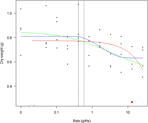
Green provided figure 1 as an example where concentration–response modeling was untenable, suggesting that the high coefficient of variation of the control group made 10% effect concentration (EC10) “estimation absurd” but nevertheless provided a point estimate of the EC10 of 0.39 g/ha and a 95% confidence interval of 0.007 g/ha to 22.8 g/ha 1. Green's preferred measure, the NOEC, was estimated using Williams' test procedure 5 to be 0.103 g/ha 1. The only way we could obtain the same result using Williams' test was by using a 0.56 level of significance. At the more usual 0.05 level of significance, the NOEC for our digitized data did not exist using William's test procedure, although using Dunnett's test a NOEC of 13.13 g/ha was obtained. Closer inspection of the data suggests the existence of a possible outlier indicated by the solid red square in Figure 1. Removing this single observation and rerunning the analysis did not alter the outcome of Williams' test but did result in a nonestimable NOEC using Dunnett's test. Rather than convince us that the NOEC is a good measure, the preceding analysis has reinforced our view that this statistic, as a measure of toxicity, is fundamentally flawed. To begin with, although the relatively high levels of variation in the response result in wider confidence intervals for model-based predictions, this extra information (uncertainty in the estimates) is at least available. One of the more severe shortcomings of the NOEC is that it has no statement of precision 6.
We are also troubled by the reporting of the NOEC. The NOEC is critically dependent on the level of significance chosen by the researcher, and this should be reported. Another disturbing aspect of the preceding analysis is that the ability to even estimate the NOEC using Dunnett's test procedure depended solely on whether a single observation was included or excluded in the analysis. As we demonstrate below, our fitted model is also affected by this single aberrant observation but in a way that is completely transparent and obvious. Indeed, the ability to “visualize” the fitted concentration–response relationship is 1 of the main strengths of the procedure, a characteristic not shared by the ANOVA/NOEC method.
Using the drc package in R 7, we have fitted a 4-parameter exponential threshold model 8, 9 both with the aberrant data point included (red curve in Figure 1) and excluded (blue curve in Figure 1). The “leverage” or influence of the aberrant observation indicated by the solid red square in Figure 1 can be assessed formally by comparing the change in the residual sum of squares between the 2 fits. The p value in Table 1 confirms that this single data point has accounted for a significant change in the residual sum of squares. The NEC estimated using the model fitted to the reduced data set is 0.41 g/ha, which is very close to Green's EC10 of 0.39 g/ha, although our own estimate of the EC10, using a 4-parameter log-logistic function (resulting in a fitted curve similar to that reported by Green 1), was 0.59 g/ha.
| Model degrees of freedom | Residual sum of squares | Degrees of freedom | F | p | |
|---|---|---|---|---|---|
| Model 1 | 40 | 0.83713 | |||
| Model 2 | 39 | 0.59885 | 1 | 15.5184 | 0.0003 |
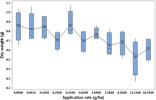
In any event, none of these model-based estimates agree with Green's NOEC of 0.103 g/ha or the Dunnett NOEC of 13.13 g/ha, both of which fail what we call the “common-sense test.” By this we mean, Does a visual inspection of the NEC estimate in relation to the overall characteristics of the concentration–response relationship look “reasonable”? A NOEC of 13.13 g/ha clearly fails this test, while a NOEC of 0.103 g/ha appears to be too low and is no doubt influenced by the “sawtoothing” response commencing at this point (Figure 2). The most accurate description of the concentration response appears to be that one does not exist for this particular data set.
Another modeling “roadblock” cited by Green 1 is the analysis of multivariate categorical data such as those generated by histopathological studies. In the next section (A Regression Model for Histopathological Severity Scores) we demonstrate that this is not true and introduce a new, novel approach for analyzing such data.
A REGRESSION MODEL FOR HISTOPATHOLOGICAL SEVERITY SCORES
One of the claimed benefits of the NOEC is that it can be computed in instances where a suitable (regression) model does not exist 1, 2. As we have argued previously (The No Observed Effect Concentration Fallacy), this assertion is simply not true; and as our analysis of the data in Figure 1 shows, there are times when the converse is true. Green cites the analysis of histopathological severity scores as an example of a “response(s) for which no suitable regression models are available” and contemplates “whether an ECx can be defined for such scores that correspond in a meaningful way to ECx in other contexts” 2. Although our work in this area has only just commenced, there is no reason why a model-based approach cannot be used for the analysis of histopathological data, as the following Example analysis demonstrates.
Example
Green et al. note that there has been increased interest in the use of histopathological data in aquatic ecotoxicology studies, with several international agencies currently collaborating to investigate their utility in studies of endocrine-disrupting chemicals 10. The nature of the data generated by such studies indeed poses new challenges for the ecotoxicological community. In contrast to the usual concentration–response experiments, there is now no single endpoint that is either observed (e.g., mortality) or measured (e.g., growth rate) as a function of an increasing chemical concentration. Instead, study subjects in 1 of k concentration groups are assigned an integer severity score to indicate the degree of “effect.” For example, a 5-point severity scale might use 0 to indicate no effect, 1 for minimal effect, through 4 for severe effect 10. Aggregation of this data produces a familiar cross-tabulation, as shown in Table 2.
| Severity score | |||||
|---|---|---|---|---|---|
| Concentration group | 1 | 2 | . . . | m | Row totals |
| x1 | f11 | f12 | f1m | f1 • | |
| x2 | f21 | f22 | f2m | f2 • | |
| . . . | |||||
| xk | fk1 | fk2 | fkm | fk • | |
There are numerous test procedures and modeling tools available for the analysis of these “contingency tables” (Table 2), although most are not aimed at teasing out information which is important in an ecotoxicological setting, such as the NEC or EC10. The most familiar of these procedures is the chi-squared contingency table test, which is an omnibus test of the hypothesis that the row and column classifications are statistically independent. In the current setting, a significant result of this test limits the researcher to concluding that severity rankings are related to concentration without being able to say anything further about the nature or form of the underlying response-generating mechanism.
Although Green et al. make an important contribution to the analysis of concentration–severity data of the type shown in Table 2, their method still focuses on the identification of NOECs for each severity category, with the minimum of the collection of NOECs claimed to be a measure of overall toxicity 10. As with conventional NOECs, these values are restricted to being selected from 1 of the k discrete classes in Table 2 and therefore are not immune to the same limitations that have faced ecotoxicologists for the last 30 yr.
 , for concentrations not exceeding the NEC is the same as the probabilities for the concentration group 1 (the control dose),
  ; 2) for concentrations exceeding the NEC, elements of the probability vector increase from left to right within a given concentration group and increase with increasing concentration. These features address issues identified with existing methods that do not account for a concentration–response relationship or acknowledge the fact that subjects exposed to higher concentrations tend to have more severe findings 10. The complete model is thus
 (1)
(1) (2)
(2) (3)
(3)
| Severity | ||||||
|---|---|---|---|---|---|---|
| Concentration | 1 | 2 | 3 | 4 | 5 | n |
| 0.0 | 38 | 17 | 11 | 2 | 0 | 68 |
| (0.500) | (0.300) | (0.150) | (0.050) | (0.000) | ||
| 0.0625 | 29 | 18 | 6 | 1 | 0 | 54 |
| (0.500) | (0.300) | (0.150) | (0.050) | (0.000) | ||
| 3.5 | 24 | 18 | 14 | 9 | 7 | 72 |
| (0.320) | (0.243) | (0.181) | (0.138) | (0.118) | ||
| 6.25 | 12 | 7 | 8 | 10 | 12 | 49 |
| (0.188) | (0.190) | (0.193) | (0.203) | (0.226) | ||
| 13 | 12 | 10 | 12 | 26 | 26 | 86 |
| (0.067) | (0.104) | (0.161) | (0.254) | (0.413) | ||
| 26 | 1 | 2 | 4 | 13 | 42 | 62 |
| (0.007) | (0.021) | (0.064) | (0.205) | (0.703) | ||
- a Numbers in each row generated using Equation 1 with sample size n and probabilities given in parentheses.
An important feature of this model represented by Equation 2 is the autoregressive nature of the vector of probabilities for concentrations exceeding the NEC, which is used to ensure that the second property above holds. Also note that the NEC for this model is γ.
The probabilities given in Table 3 were generated using the model above with the following parameter values: α = 0.2; β = [0.1257 0.087 0.04834 0.009675 -0.029]; and γ = 1.875.
Inspection of the generated probabilities (Table 3) or a plot as a function of concentration and severity (Figure 3) shows an increased likelihood of a more severe score with increasing concentration.
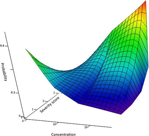
The frequencies given in Table 3 represent a single realization from Equation 1 with  given in Table 3 and
  . We next present 2 modeling approaches to estimate the NEC for these data. The first is an implementation of the Bayesian approach described in Fox 9 (Bayesian estimation). A second, and new strategy is to utilize ordination methods commonly used in the analysis of multidimensional ecological data (Model fitting using ordination techniques).
Bayesian estimation
Implementation of a Bayesian approach to model fitting using software tools such as OpenBUGS, JAGS, or STAN is relatively straightforward. This involves the following steps: 1) set prior densities on the parameters {α, βi, γ}; 2) obtain an empirical estimate of the control dose probability vector as  ; 3) populate the remainder of the matrix of probability estimates
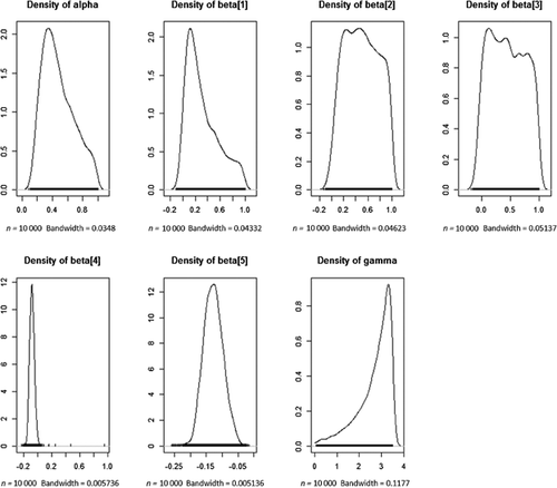
  using Equations 2 and 3; 4) compute the likelihood function based on Equation 1; and 5) using Markov chain Monte Carlo techniques, generate samples from the empirical posterior distributions of {α, βi, γ}. Based on a 10% sample from 100 000 iterations of the above procedure, a point estimate of the NEC of 2.69 was obtained. The 95% region of highest posterior density was the interval [1.084; 3.50]. Empirical estimates of the posterior densities for all model parameters are shown in Figure 4. The shape of the empirical posterior densities in Figure 4 suggests that there are many combinations of parameter values other than the true values that provide a reasonable description of the data in Table 3. Nevertheless, the NEC has been estimated reasonably well, with the true value of 1.875 falling in the middle of the highest posterior density interval.
Model fitting using ordination techniques
As noted earlier in the Example, a difficulty posed by the data structure in Table 2 is that the response is a discrete multivariate random variable. Vegetation ecologists frequently deal with this kind of data, which are often presented as a “community matrix.” In this form, taxa form the columns and sites form the rows, with cell entries being either 0/1 (presence/absence) data, numeric counts, or some other measure such as cover percentages or cover classes. One of the aims of collecting such data is to discover spatial–temporal patterns or clustering among species or to model the response as a function of other landscape attributes such as slope, aspect, and soil properties. A variety of statistical tools and techniques are used for these purposes, and many of these are described in the R packages labdsv, mefa, and vegan 7. A common strategy used to facilitate the modeling, visualization, and interpretation of these multivariate data is to reduce the dimension of the sample space with minimum sacrifice of information contained in the original sample. Similarity measures provide 1 way of achieving this. One commonly used measure is the Bray-Curtis similarity index 11. Like a correlation coefficient, this index has a simple interpretation, with values ranging between 0 (2 “sites” having no species in common) and 1 (2 “sites” sharing all species). For the present example, we have computed values of the Bray-Curtis index by comparing the pattern of severity scores at each non-0 concentration to the pattern of severity scores for the control group (Table 4).
| Concentration | Bray-Curtis index relative to control |
|---|---|
| 0 | 1.000 |
| 0.0625 | 0.869 |
| 3.5 | 0.771 |
| 6.25 | 0.496 |
| 13 | 0.455 |
| 26 | 0.138 |
The results from fitting a log-logistic model to the Bray-Curtis data (Table 4) using the drc package in R 7 are shown in Figure 5.
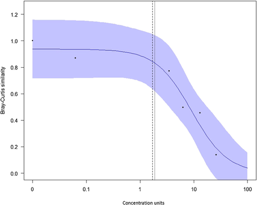
The appeal of this procedure is evident, with the high-dimensional data of Table 3 reduced to a more familiar concentration–response type plot (Figure 5) and model from which any ECx can be obtained. A Bayesian fit of the exponential-threshold model 8, 9 gave an estimated NEC of 2.194 with a highest posterior density interval of 0.08 to 17.9. Although still in its infancy, this modeling approach appears to provide a viable mechanism for fitting concentration–response models to histopathological data. Although the estimated EC10 of 1.7 from Figure 5 is very close to the true NEC of 1.875, this is coincidental. We have long argued that “the NOEC is an estimate of a [NEC] for which x = 0 is axiomatic” 3 and therefore comparisons between a NOEC and other summary statistics are meaningless. Yet the temptation to draw comparisons seems irresistible, with papers continuing to be published comparing NOECs and ECs 12, 13.
What is clear is that after more than 30 yr of debating the relative merits of NOECs 14, NECs, and ECxs, we still have not reached a new consensus. De Bruijn and Hof were correct when they noted back in 1997 that even if the ECx was to replace the NOEC, it would take many years for the transition to occur 15. Despite progress with model development for the estimation of a NEC such as those identified by Pires et al. 8 and newer estimation strategies such as those in Fox 9, researchers seem wedded to the NOEC concept or the derivation of a single estimate to represent toxicity (ECx). For example, Pires et al. 8 identified 3 nonlinear threshold models and described methods of estimating the NEC but felt compelled to ask “how do the estimated NECs and the NOECs compare with the same data” 8.
It is time to move on. It is also time to take positive steps to phase out NOECs and for the international ecotoxicology community to heed the many calls to model the concentration–response relationship and to use the complete curve rather than reduce it to a single metric. If this relationship must be reduced to a single metric, then the overwhelming weight of scientific opinion is that NECs and ECxs are the preferred toxicity measures. We understand there remain open questions, such as the choice of x, but believe this should be based on a broader range of considerations that include (as a function of x) the following: ecological consequences, environmental benefit, compliance cost, implications for management, and economic impact. A more productive line of investigation would be to adopt the recommendation that “guidelines should be developed to indicate when which model should be chosen” 16.
CONCLUSIONS
In the present study we have provided a counterpoint to recently promoted views that the NOEC is a credible toxicity measure. The debate about the usefulness, utility, and desirability of using NOECs has been going on for over a quarter of a century, and while diversity of views, stress testing, and critical appraisal are central to science, we believe the time has come to give effect to the many and sustained calls to shelve this metric.
We are unconvinced by claims that certain “problematic” toxicity data justify the retention of NOECs. As we have demonstrated, it is possible to develop a meaningful concentration–response modeling and estimation framework for multivariate severity score data. Admittedly, this has entailed some reasonably advanced mathematical and statistical skills, but that should not be used as an argument to support the continued use of the inferior NOEC. Indeed, it is for precisely this reason that we have actively promoted the formalization of a statistical ecotoxicology subdiscipline to nurture and support novel and creative statistical development in ecotoxicology 3.
Jurisdictions around the world (US Environmental Protection Agency 17, European Union 18, 19, Environment Canada 20, Australian and New Zealand Environment and Conservation Council/Agricultural and Resources Management Council of Australia and New Zealand 21) have all supported Pack's 1993 recommendation that “EC point estimation (i.e., percentiles of the concentration response curve) should become the preferred option” 22. Yet here we are in 2016 having made little progress toward implementation of that objective, with small but vocal NOEC advocates pushing against the tide of scientific opinion. Perhaps it will take a Global SETAC initiative to organize a Paris-style convention 23 to hammer out a deal and to have “member nations” sign up to the ratified plan. Until that time, we see a future no different from the past, with NOECs continuing to be used interchangeably with ECs.
Acknowledgment
We are grateful to the anonymous reviewers whose suggestions greatly helped improve the clarity of the final manuscript.
Data availability
Data are available from the corresponding author at [email protected].


