Effective monitoring of drilling tool condition is crucial in mechanical metal cutting to prevent tool failure, maintain machining accuracy, and ensure superior surface finish quality. Tool breakage or wear can cause catastrophic machine downtime, reduce dimensional accuracy, and deteriorate the surface finish of machined parts, thereby impacting productivity and operational costs. To address these challenges, this paper presents a data-driven fault diagnosis approach that leverages vibration signal analysis for real-time condition monitoring of drilling tools. In this study, vibration signals were collected using a piezoelectric accelerometer mounted on a CNC drilling machine during operations involving both new and worn tools. Various stages of tool wear were examined to capture comprehensive vibration data reflective of different fault conditions. Statistical features were extracted from these vibration signals, including measures such as mean, variance, kurtosis, and skewness, to characterize the tool's health status effectively. For fault diagnosis, a best-first tree classifier was employed due to its robustness and interpretability in handling features and obtained accuracy of 96.23% that validates the potential of the proposed data-driven approach. The proposed method offers several advantages, including non-invasiveness, real-time applicability, and scalability across different manufacturing setups. By integrating vibration-based condition monitoring with machine learning techniques, the approach facilitates early fault detection, enabling predictive maintenance strategies that can significantly reduce unplanned downtime, extend tool life, and improve overall manufacturing productivity. In conclusion, the paper demonstrates that a data-driven, vibration-based fault diagnosis system combined with an effective classification algorithm can serve as a practical solution for continuous monitoring of drilling tool conditions, thereby supporting enhanced operational efficiency in metal cutting industries.

1 Introduction

Drilling is a joint operation that accounts for approximately 40% of the cutting process in industry [1]. When a drilling tool is constantly used, it wears down, affecting the workpiece's dimensional accuracy and surface finish. A worn drill tool can no longer create holes in the required workpiece specifications [2]. With any tool, progressive wear and tear can occur after a specific period of use. A tool reaches its service limit during progressive wear owing to flank or crater wear. This type of wear is classified as normal wear. In addition, there is potential for uneven tool wear, which can be eliminated by carefully selecting tool materials and cutting settings. Owing to the fragility of the tools, there is a possibility of breakage and changes in the machine's operating parameters, resulting in complete failure and sometimes even small pieces falling off the cutting edge. Constant tool maintenance can prevent sudden breakdowns. Fractures or cutting-edge splits cannot be treated in this way [3, 4]. The diameter of twist drills generally ranges from 1 to 20 mm. Twist drills are susceptible to failure: breaking, chipping, and extreme wear. Drill wear and failure directly affect the parameters of the drilling process. A worn drill produces vibration signals that can be used to define the drill conditions. Drilling applications must improve effective methods for the online detection of tool wear and breakage [1]. Tool wear is a concern in machining operations because it reduces the useful life and effectiveness of the cutting tools. This phenomenon directly influences the surface quality and dimensional accuracy of the machined surface, consequently impacting the metal-cutting industry's productivity [5]. A 20% machine downtime in manufacturing has been attributed to tool wear [6]. Moreover, the expenditure associated with cutting tools and tool changes typically accounts for approximately 3%–12% of the overall machining expenses. Implementing a robust monitoring system has decreased wear and damage to machine tools and reduced downtime and lead time [7]. Nakandhrakumar and Dimla identify tool wear or failure in real-time, which presents a significant challenge in the pursuit of automated optimization. Continuous supervision of the drill tool is necessary to facilitate timely and appropriate replacement of the tool for which specific indicators are required. In the past, identifying and discovering abrupt failures of the cutting tool or the onset of failure mechanisms was challenging. The task was primarily performed by machine operators who relied on their industry experience or employed mathematical cutting-process models. The operator decides to switch tools after determining their performance. Consequently, cutting tools were found insufficiently or excessively utilized, failing to accommodate the intricate and heterogeneous nature of metal cutting operations, as demonstrated in previous studies [8, 9]. Therefore, various sensory signals are utilized to assess the state of the cutting tool to prevent such scenarios [10, 11]. The field of fault diagnosis, commonly known as condition-based maintenance (CBM), encompasses a range of maintenance methodologies that employ various techniques to assess the current state of the equipment and develop maintenance schedules. This procedure involves regular or continuous examination of the equipment's health. Implementing fault diagnosis in tool operations has improved asset safety and reduced operating expenses. Several parameters have been identified as influential in determining the tool conditions during the machining process, including vibration, temperature, acoustic emission, cutting force, and spindle current. To enhance machining operations and minimize tooling costs, it is imperative to conduct fault diagnosis of the tool. Utilizing a worn tool for machining operations has the disadvantage of generating friction between the tool and workpiece, leading to heightened power consumption [12-14]. To ensure the tool performs at its best, metal cutting operations include the methodical examination and assessment of the cutting process, tools, and workpieces. Nevertheless, exaggerated power takeoff, imprecise tolerances, and diminished surface finish harm the machine tool and injure the operator. Consequently, implementing a tool-condition monitoring system is essential [15-18].

The literature review highlights the need to characterize faults arising from unknown vibration movements beyond conservative machining parameters. Vibration signals acquired through accelerometers provide reliable data for onboard fault diagnosis, with this study focusing on time-domain analysis. While statistical feature extraction using decision trees is efficient, real-time tool fault classification via supervised tree-based classifiers remains underexplored. This research aims to monitor drilling tool faults using a data-driven intelligent approach, requiring fault characterization based on vibration data, statistical methods, and machine learning.

2 Tool Condition Monitoring Approaches

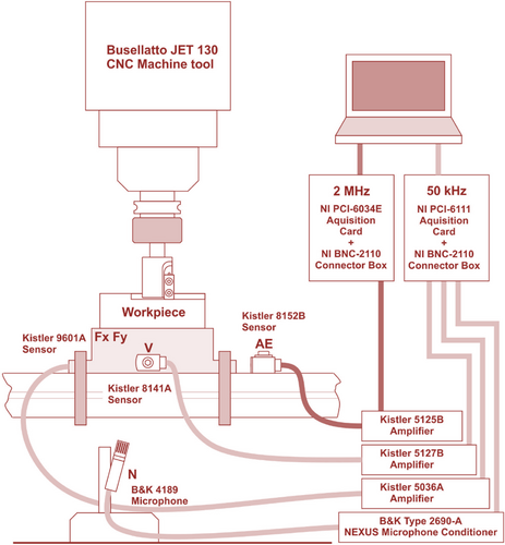
Machine tools are crucial in modern production systems. Monitoring tool wear helps to reduce sudden failures, and researchers have proposed several methods. Monitoring the condition of tools can reduce machine tool damage and unexpected downtime. The tool condition monitoring system comprises a set of sensors, signal amplifiers, and a data-gathering system to monitor the drilling process. Because the sensor is the primary component, it should be positioned closest to the tooltip and the desired position. Then, the signal must be received to obtain valuable information from the sensors. The data acquisition system analyzes the signal received from the sensor and displays the results on a computer [19-21]. The area of online supervision of manufacturing processes has seen an increase in the number of researchers owing to the increased requirement for process automation for unmanned production. Therefore, extensive research has been conducted worldwide on online tool condition monitoring systems [22]. Monitoring of tool wear and defects requires the development of susceptible, accurate, and reliable methods that can be classified as “direct” or “indirect” [23]. Figure 1 shows the framework of the tool-condition monitoring system to identify tool wear in the machining process using a data acquisition and machine learning approach.

Details are in the caption following the image — **FIGURE 1**
Open in figure viewer PowerPoint

Sensor-based tool condition monitoring [19].

2.1 Direct Methods

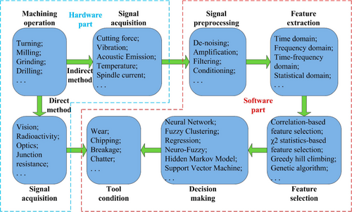
Direct approaches rely on measuring tool wear directly through proximity sensors, vision systems, optical signals, radioactivity, and electrical resistance. These techniques usually involve assessing the volumetric loss of the cutting tool material. These are generally “offline” methods, as the measurement can only be made when the tool no longer has a cutting edge. The advantage of direct tool-wear approaches is that they can capture the geometric changes caused by tool wear. However, direct measurements are less favorable because the cutting area is inaccessible [11]. The two main disadvantages of offline methods are that they are time-consuming owing to production speed and advanced premature failures. Additionally, the tool was in a cut that could not be detected. However, owing to the difficulties in implementing direct methods, many researchers have been able to determine the tool wear during the process by measuring parameters closely related to tool wear [7, 12]. Figure 2 shows a schematic of direct and indirect TCM.

2.2 Indirect Methods

Indirect techniques rely on variables related to wear and are monitored during cutting. In the indirect approach, the state of the cutting tool is predicted using parameters that can be predicted from the sensor signal output rather than being directly measured. The indirect tool-condition monitoring system consists of four stages.

Data Collection: Signals are gathered from sensors, including force, vibration, temperature, motor current, and sound emissions.
Signal Processing and Feature Extraction: The collected signals are processed to extract relevant features concerning the time domain, frequency domain, and so forth.
Tool wear estimation: Various data-driven intelligence algorithms estimate tool wear.
Decision-Making Algorithm Development: A decision-making algorithm is recognized based on sensor data to control tool wear [7, 10, 12].

In recent years, data-driven event-triggered Adaptive Dynamic Programming (ADP) control has emerged as a powerful framework for optimizing control performance in complex nonlinear systems. This approach enables systems to learn optimal control policies directly from data, while event-triggered mechanisms reduce unnecessary computations and communication by updating control actions only when needed. By integrating these methods, adaptive control becomes more efficient and scalable, especially in dynamic environments like mechanical metal cutting. The application of such intelligent control frameworks in drilling tool monitoring can significantly enhance fault diagnosis accuracy and system responsiveness under uncertain and varying operational conditions. Zhang et al. [24] introduced an event-triggered ADP using a single critic network and experience replay to reduce computational overhead. Similarly, Hu et al. [25] proposed adaptive event-triggered control with auxiliary dynamic variables to ensure asymptotic stability in discrete-time systems. Chu et al. [26] addressed parameter uncertainties in nonlinear dynamics by combining adaptive control with a simple event-triggering mechanism, ensuring the boundedness of system signals without Zeno behavior. Liu et al. [27] extended this by developing an ADP-based control strategy that accommodates asymmetric input constraints and disturbances while maintaining stability. Zhao et al. [28] demonstrated that event-triggered ADP could also be effectively applied in multi-agent systems to reduce communication loads and maintain consensus. Liang et al. [29] proposed a learning-based event-triggered guaranteed cost control framework using integral reinforcement learning to manage completely unknown systems. Peng et al. [30] presented an identifier-critic learning model that reconstructs system dynamics for optimal event-triggered control in unknown nonlinear environments. Lastly, Siddique et al. [31] introduced a reinforcement learning that optimizes control and communication policies, reducing computational burden while keeping performance robust. Thus, the growing potential of event-triggered, data-driven ADP methods in intelligent manufacturing systems has become a need, where system complexity, variability, and computational efficiency are critical considerations.

3 Process Parameters and Signal Acquisition

The measurement of process parameters, including torque, vibration, cutting force, and acoustic emission, is required during drilling tool condition monitoring at each stage of the tool's life. The process parameters must be obtained using an appropriate sensor. The process parameters are described in the following subsection.

3.1 Measurements of Torque, Drift Force, and Feed Force

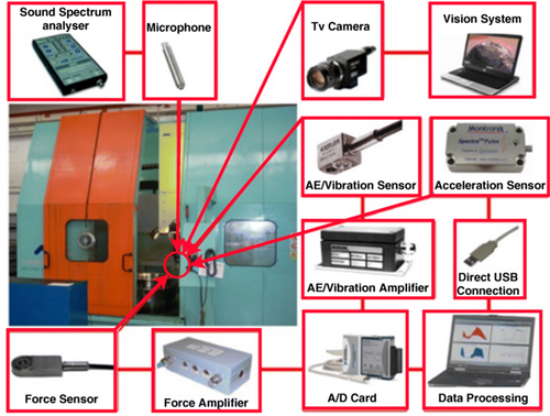
Monitoring forces during cutting processes provides a rational and practical basis for supervising cutting tool wear. The gradual increase in friction between the tool and workpiece leads to a corresponding increase in the cutting force, which is further intensified by the wear and tear of the tool, as observed in previous studies. During the drilling process, torque, drift forces, and feed can be observed. Monitoring this task is necessary because of the anticipated alterations in the tool's forces, wear, and tear. In contrast to other cutting tools, the wear of drill tools manifests differently because of the somewhat asymmetric nature of the drill bit, which is attributable to manufacturing tolerances. The study initially observed uniform wear of one lip until the heights of both lips were equal. After drilling, the second lip was cut. This process persisted until there was no further clearance at the margins. If the drill tool is not stopped, gradual adherence of the drill bit to the workpiece could lead to failure. The monitoring of the drift forces becomes apparent by observing the progression of this type of wear. The research conducted by [32] demonstrated an association between the assessment of thrust force and torque and the waviness of the hole surface. Consequently, the change in waviness as a function of tool wear is understood, and the study indicates that the thrust force is prioritized over the torque because it provides a more precise indication of tool wear. Several studies have employed torque, feed force, and strain as the process parameters for measurement [33-36]. The assessment of lateral forces perpendicular to the tool axis is quantified via strain gauge sensors to monitor the aforementioned parameters continuously. One of the analyses employed strain gauges positioned at the spindle to quantify thrust force [37]. In previous studies, researchers compared the torque, drift, and feed force with the measurement of ultrasonic vibration [38]. The proposed patented method for predicting the wear and failure of a drill bit involves conducting both static and dynamic torque measurements through the measurement of eddy currents. The method utilized in this study entailed precise placement of the sensor at a distance of 0.2–0.5 mm from the drill shank. The proximity of the sensor to the drill shank and the material composition of the drill significantly influence the torque measurement [39]. Several theories have proposed minimal to no significant effects on the cutting forces. An examination featuring a copper alloy and model, as referenced in [34], highlighted the mathematical formulations delineating the relationship between the thrust force and torque and the feed per revolution, drill diameter, and flank wear variables. A study conducted to evaluate the applicability of the test determined that the variation in cutting speed across the range did not significantly impact the strength of the work material. A strong correlation was observed with the regression formulae of the test data without the spindle's rotational speed. The coefficient of determination (R²) for the feed force and torque was found to be 0.94 and 0.97, respectively. It has been demonstrated that accurate estimation of tool wear requires knowledge of the thrust force and other cutting parameters, particularly for larger tool wear. The variation of tip life was investigated, and it was concluded that the hardness of the workpiece influences it. This conclusion was based on tests performed on workpiece materials with different hardness values. This made it possible to develop torque and thrust formulas that depended on the Brinell hardness of the workpiece material, tip diameter, feed per revolution, average flank wear, and cutting-edge radius [34]. It has been hypothesized that using multiple high-hardness bits affects the drill life much more than in a scenario where industrial activity relies on only a few low-hardness bits. This is observed in many industrial operations where tip failure depends on various high-hardness parts, which ultimately explains the wide variation in tip life observed under industrial conditions. Some test results are difficult to implement, for example, in industrial castings. According to the derived concept, the workpiece also influences the magnitude of the torque and thrust forces. To diagnose flank wear based on the amplitude of the thrust force or torque, the fluctuation in workpiece hardness must be maintained within 5% of the mean hardness value because this will affect the calculable variation in thrust force caused by any change in flank wear. It was concluded that torque or thrust measurements should not be used to monitor drill wear until a thorough workpiece hardness tolerance is ensured. The experimental setup, which included a multi-sensor arrangement, is shown in Figure 3.

In this study, the thrust and torque parameters predicting various errors in the drilling tool were considered, and these signals were also extracted [40]. This work investigated the time-frequency domain analysis for extracting signals using a multisensory method for drilling wear monitoring. In addition, the frequency domain correlates better with tip wear than the time-domain analysis, which considers the torque, force, and two strain sensors [41]. In these experiments, a hidden Markov model technique was used to classify tool wear by measuring torque, thrust, and shaft power [42]. This study considered the traction force to classify drill tool conditions using statistical parameters, fuzzy logic, and a neuro-fuzzy system (ANFIS) to predict drill tool conditions [43]. Flank wear monitoring has been studied concerning cutting conditions, drill diameter, thrust, torque, and chip thickness to predict tool wear using a fuzzy backpropagation neural network [44]. This study extracted thrust force and torque signals using a Kistler piezoelectric dynamometer. Drilling tool error prediction was performed using a fuzzy rule-based model [45]. A radial drilling machine performed experiments using HSS drilling tools of various diameters. The signals were extracted from the piezoelectric dynamometer and accelerometer sensors. Tool wear prediction was performed using the ANN ensemble method [46]. This study predicted tool wear/breakage using a neural network algorithm. The Ni-based superalloy drills of Inconel 625 and 5.95 mm uncoated cobalt steel drill were used for drilling [47]. This study performed frequency-domain analyses of the thrust and torque signals. Tool-wear prediction was performed using an artificial neural network method [48]. In another study, traction and torque signals were measured using a dynamometer. Tool-wear prediction was achieved using the Adaptive Neuro-Fuzzy Inference System (ANFIS) algorithm [49]. Table 1 presents the specifications for various workpieces, tools, and machining parameters, along with the use of a cutting force sensor, and Table 2 outlines cutting force sensor specifications for the drilling process.

TABLE 1. Summary of workpiece, tool specifications, and machining parameters using cutting force sensor.

Sr. no.	Workpiece material	Typical machine type	Tool material(s)	Diameter range (mm)	Speed range	Feed range	Hole depth range (mm)	References
1	Carbon fiber reinforced polymers (CFRP)	CNC/vertical machining center	Carbide, PCD, TiN-coated	2–7.92	41–3000 rpm/170 m/min	0.025–0.2 mm/rev or mm/min	4.5–15	[50-55]
2	Mild steel	Radial drilling, CNC	High-speed steel	5–10	250–1600 rpm	0.12–0.71 mm/rev	Blind–15	[44, 49, 56]
3	Aluminum	CNC/bench drill	Tungsten carbide	1–6	3000 rpm–41 m/min	2 μm/rev–0.1 mm/rev	5–15	[53, 57]
4	Glass fiber reinforced plastic (GFRP)	Vertical milling/CNC	TiN-coated carbide	6–10	500–2500 rpm	10–500 mm/min	Blind hole	[45, 58]
5	Titanium alloys	Vertical milling center	High-speed steel	4	600–800 rpm	0.033–0.056 mm/rev	10	[59]
6	Inconel 625	Vertical machining center	Cobalt steel	5.95	400–600 rpm	0.05–0.1 mm/rev	Blind hole	[47]
7	Cast Iron	CNC machining center	High-speed steel	8	1600–1800 rpm	300–450 mm/min	20	[60]
8	Carbon steel	CNC milling/machining center	High-speed steel	6–12	16–1000 rpm/m/min	0.06–0.3 mm/rev	11.4–42	[6, 40, 41]
9	Alloy steel	CNC	Solid carbide	8	70–100 m/min	0.15 mm/rev	5	[61]
10	Melamine chipboard	CNC machine tool	Tungsten carbide	12	4500 rpm	1.35 m/min	Blind hole	[62]

TABLE 2. Summary of cutting force sensor used in drilling applications.

Sensor type	Sensitivity (pC/N or mV/N)	Temperature range (°C)	Force measurement range (kN)	References
Kistler piezoelectric dynamometers (various models, e.g., 9123, 9255B, 9257, 9271A, 9272)	∼3.6–8 pC/N or 2 mV/N	0–70/–40 to 120	±5 to ±20 kN	[40, 41, 45-47, 49-54, 57-59, 61, 62]
Kistler minidyn dynamometer (9256C2)	−26 pC/N	0–70	±250 kN	[63]
Drill tool dynamometer/other piezoelectric sensors	∼6–9 pC/N	0–70	±5 to ±15 kN	[6, 44, 45, 55, 60]
SYSCON dynamometer SI-674	NA	0–50	˜0.5 kN (500 kg)	[56]

3.2 Measurements of Vibration and Sound

Vibration is one of several techniques used for condition monitoring in rotating machinery; however, a few drawbacks have limited its application in tool condition monitoring. These include its technical sensitivity to noise during cutting processes and its potential dependence on the workpiece material, cutting conditions, and machine structure on vibration signals. Vibration measurement offers several advantages, including ease of implementation and the absence of the need for modifications to the machine tool or workpiece fixture [64]. A study was undertaken to develop vibration-based monitoring techniques for detecting breakage in small-sized drills (3 mm diameter) and wear in larger-sized drills (6 mm diameter) [1]. The vibration was calculated in both the transverse and axial orientations. It is known that vibration signals are a reliable way to track tool wear and breakage. Because the vibrating drill length in the axial and transverse modes does not vary during drilling, it can maintain a constant mode frequency. Furthermore, the work material of the drill bit remains unaffected by changes in the drill cross-sectional size concerning the natural frequencies of the transverse and axial modes, even when different drill bits of different sizes are monitored.

Moreover, vibrations in the Y and Z directions affect the torque and thrust force, which are influential factors in drilling operations. The study described in Reference [65] involved the conduction of testing using three accelerometers. In a study by the author [66], vibration measurement was employed in conjunction with thrust force to acquire a signal capable of detecting tool wear and facilitating the development of a diagnostic tool. The data were captured using a machine vision system. In principle, the measurements obtained from sound and vibration analyses may be aligned because of the transfer of mechanical vibrations from tool contact to sound on a technical level. However, external factors may affect sound measurements, potentially influencing the results. Hence, this is a drawback in the context of sound assessments.

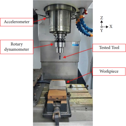
However, it is imperative to acknowledge the significance of this measurement method. Presently, operators continue to utilize auditory cues to identify tool wear and attempt to characterize the issues within the tool. After conducting a series of tests, it was found that vibration measurement was the most reliable method compared to sound measurement. The experimental findings indicated that thin drills' vibration measurements yielded a broader frequency range of 0.5–40 kHz. Specifically, a drill with a diameter of 1 mm produced vibrations at approximately 25 kHz, whereas a 3 mm diameter drill generated vibrations at approximately 7 kHz. Figure 4 illustrates the experimental setup in which accelerometer and dynamo positioning was implemented.

In this study, the wear and failure of drilling tools were monitored using the time domain, extracted frequency domain, and vibration signals. This study performed fault diagnosis by extracting vibration signals using an accelerometer. The wear of drilling tools was predicted using a logistic regression model. Wavelet packet decomposition [67] was used for feature extraction. This study investigated time-domain analysis and extracted statistical features using vibration signals. The vibration amplitude is a dominant characteristic compared to the others [68]. This study investigated the wear of drilling tools by collecting vibration signals. Time- and frequency-domain studies were also conducted. The wave properties were extracted from the received vibration signals. The Support Vector Machine (SVM), Artificial Neural Network (ANN), and Bayesian classifiers were used to predict tool wear [69]. In this study, experiments were conducted on a mild steel workpiece. High-speed steel rotary drills were used for drilling. Time- and frequency-domain analyses were conducted. Vibration signals were extracted using an accelerometer sensor. The severity of the tool wear was monitored. This study monitored the health of the online tools. Vibration signals were extracted to predict tool wear [70]. High-speed steel and tungsten carbide rotary drills were used to drill the titanium alloy workpiece. The vibration signals were obtained using a triaxial accelerometer. The lateral wear of the drilling tool was predicted [71]. In this study, vibration signals were collected, and a backpropagation algorithm was utilized to forecast the lateral wear of a drilling tool. In addition, time- and frequency-domain analyses have been conducted [72].

In this study, a mathematical model was developed to measure the lateral wear of drilling tools. Vibration signals were recorded using an accelerometer, and the time and frequency domains were analyzed [8, 19]. In this study, drilling operations on CFRP sheets, PMMA sheets, and 6061 aluminum alloys were performed using different drills. Vibration signals were obtained using a piezoelectric accelerometer. Vibration frequency versus time and acceleration versus time analyses were performed [73]. In this study, sensor synthesis analysis was performed. The drilling tool wear classification was achieved using a Support Vector Machine algorithm. This study analyzes the lateral wear of a drilling tool by extracting statistical features from the vibration data. Tool wear was classified with an accuracy of 79.56% using the K-star algorithm. Table 3 illustrates the specifications of various workpieces, tools, and machining parameters using the vibration signal sensor, while Table 4 details the vibration sensor specifications for the drilling process.

TABLE 3. Summary of workpiece, tool specifications, and machining parameters using vibration signal sensors.

Sr. no.	Workpiece material	Machine type(s)	Tool material(s)	Diameter (mm)	Speed range	Feed range	Hole depth	References
1	EN24 steel	CNC, precision milling, drilling	High-speed steel	6–6.1	450–1000 rpm	71 mm/min, 0.089–0.15 mm/rev	Blind–15 mm	[8, 19, 68, 72]
2	Mild steel	CNC, radial, conventional drills	High-speed steel	5–10	140–1160 rpm	0.02–0.71 mm/rev	Blind–15 mm	[21, 46, 56, 69]
3	Titanium alloys	CNC, drilling	HSS, tungsten carbide	4–10	600–10,600 rpm	0.033–0.4 mm/rev	Blind–10 mm	[59, 71]
4	Cast iron	CNC machining center	High-speed steel	3–8	12–1800 rpm/m/min	0.12–0.37 mm/rev	15–30 mm	[1, 60]
5	Alloy steel	CNC vertical milling	Solid carbide	8	40–100 m/min	0.07–0.15 mm/rev	5–16 mm	[15, 61]
6	Aluminum	Bench drill	Tungsten carbide	1	3000 rpm	2 μm/rev	5 mm	[57]
7	Carbon steel	CNC vertical machining center	High-speed steel	8–12	500–1000 rpm	10–45 mm/min	30–42 mm	[40]
8	Carbon fiber composites	Vertical machining center	Polycrystalline diamond	6	113–170 m/min	80–110 mm/min	5 mm	[54]
9	Melamine chipboard	CNC machine tool	Tungsten carbide	12	4500 rpm	1.35 m/min	Blind hole	[62]
10	Stainless steel	CNC vertical mill	High-speed steel	10	9.4–16 m/min	0.109–0.135 mm/rev	Blind hole	[2]
11	AISI 1045 steel	CNC gundrill	Carbide	10	2228–2389 rpm	0.023–0.029 mm/rev	120 mm	[70]

TABLE 4. Summary of vibration sensors used in drilling applications.

Sensor type	Typical sensitivity (mV/g or pC/g)	Temperature range (°C)	Frequency/range (g)	References
Piezoelectric accelerometers	10–100 mV/g; 3–10 pC/g	−74 to 250	±50 g to ±500 g	[15, 46, 56, 69-73]
MEMS accelerometers	∼2048 LSB/g, ˜350 mV/g	−40 to 120	±2 g to ±16 g	[8, 21, 40, 73, 74]
PCB/Kistler accelerometers	Mostly 100 mV/g	−54 to 121	±50 g to ±1000 g	[1, 19, 54, 59, 61-63, 69, 71]
Bruel & Kjaer accelerometers	10 mV/g to 10 pC/g	−50 to 250	±76 g to ±500 g	[15, 46]
Others/generic sensors	100 mV/g (mostly)	−40 to 85	±2 g to ±6 g	[2, 8, 19, 21, 40, 60]

3.3 Measurement of Acoustic Emission and Ultrasonic Vibration

Assessments have been conducted on applying ultrasonic vibrations (UEs) in the frequency range of 20–80 kHz for tool breakage detection in various metal cutting operations, including drilling [75]. AE suffers from substantial attenuation and multipath distortion due to bolted joints, which are frequently present in machine tool construction and limit the mounting location to somewhere close to the tool or workpiece. The transducer can be positioned considerably farther from the chip manufacturing zone when a lower-frequency signal is used for UE analysis because it causes less noticeable attenuation and distortion. In the low-frequency vibration range, the prominence of the structural modes was observed at frequencies below 20 kHz. A typical approach is to compare various frequency bands in the amplitudes of this range. Tool wear and breakage are process irregularities indicated by specific differences in the relative vibration strength in these bands. Although this method offers the same advantages of remote transducer positioning as the UE method, it is noticeably more vulnerable to the effects of machine and tooling differences. The variability of structural modes in response to machinery movement, loading, temperature fluctuations, and tooling necessitates empirical tuning of this approach each time the process changes. The frequency range utilized for analyzing a given UE is characterized by closely spaced structural modes that collectively exhibit the behavior of a pseudo-continuum. With machine movement, loading, and other factors, no individual resonances can migrate out of the analysis band [22]. According to the authors, acoustic emission occurs within the 10–70 kHz frequency range, and a sensor with a nonlinear frequency response is referred to as an AE sensor. The efficacy of ultrasonic vibration surpasses torque, feed, and drift force measurements in detecting tool wear and failure during drilling operations [22]. An identical sensor was employed for measurements within the 1–5 kHz frequency spectrum, which is typically associated with mechanical vibration. The occurrence of acoustic emission is characterized by the generation of small displacements on the surface of a material for various reasons [76]. This phenomenon is caused by stress waves that spread when energy is suddenly released inside a material or surface. The 200 kHz sensor was used in the experimental tests to identify tool wear, and an 800 kHz sensor was used to identify tool breakage. A broadband sensor was deployed to identify the optimal frequency range for subsequent analyses. The study by [76] involved recording acoustic emissions in a broad frequency range of 100–1000 kHz for monitoring tool wear. Figure 5 demonstrates the experimental setup in which the AE sensor was instigated.

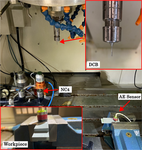
This study classifies drilling tool wear using a fuzzy neural network (FNN) approach. Here, acoustic emission signals were obtained, and the wave characteristics were extracted. Hardened steel workpieces were drilled using high-speed steel drilling tools [77-79]. In this study, wavelet analysis was performed to monitor the conditions of the drilling tools using acoustic emission signals. The glass/phenolic polymer composite material was drilled using a high-speed steel drill [80]. Flank wear tests were performed using a carbide tip. Steel plates were drilled. In this case, frequency domain analysis was performed using the acoustic emission signals and the tool wear classification algorithm K Means [81]. This study investigated the damage caused by high-speed steel drilling tools. Acoustic emission signals were obtained, and frequency and time-frequency domain analyses were performed [79]. In this study, the wear of carbide drilling tools was investigated. Titanium plates were drilled. Acoustic emission signals were obtained, and statistical, spectrum, and wavelet packet analyses were performed [50]. Using a backpropagation learning technique, this study employed the time domain and wavelet packet transform to forecast drilling tool wear. Acoustic emission signals were obtained for different tool wear states. A high-speed steel drill was used, and the workpiece to be drilled was selected as mild steel [82]. This study obtained acoustic emission and torque signals under different wear states of drilling tools, and a time-domain analysis was performed. In this case, a high-speed steel drill was used, and the workpiece was drilled from SAE 1040 steel [83]. Table 5 illustrates the specifications of various workpieces, tools, and machining parameters using AE sensors, while Table 6 provides the acoustic emission sensor specifications for the drilling process.

TABLE 5. Summary of workpiece materials, tools, and machining conditions using AE sensors.

Sr. no.	Workpiece material type	Specific material(s)	Tool material(s)/type	Machine type	Speed and feed (range)	Hole type	References
1	Metallic (ferrous & alloys)	Steel (SAE 1040), mild steel, quenched steel, alloy steel, CGI	HSS, solid/cemented carbide	Vertical, CNC, machining centers	300–1250 rpm/0.07–0.25 mm/rev	Blind/through	[15, 61, 79, 81-84]
2	Metallic (non-ferrous)	Aluminum, Al-5% SiC MMC	Tungsten carbide, HSS	NC drill, CNC micro machining	600–3000 rpm/2 μm/r to 0.17 mm/rev	Through	[57, 78]
3	Composites—polymer & fiber reinforced	CFRP + Ti alloy, GFRP, epoxy, phenolic, glass composites	HSS, Ti-coated carbide, carbide	VMCs, milling machines, drill machines	260–2700 rpm/10–125 mm/min	Mostly blind	[58, 80, 85, 86]
4	Polymeric and wood-based	Melamine chipboard, araldite epoxy resin	Tungsten carbide, HSS	CNC, drill machines	315–4500 rpm/1.35 m/min	Blind	[62, 87]

TABLE 6. Summary of acoustic emission sensors used in drilling applications.

Sensor type	Typical sensitivity	Temp range (°C)	Frequency range	References
Kistler AE sensors (8152 series)	48–57 dB (ref 1 V/(m/s))	−55 to 165	50–400 kHz	[15, 61, 62, 80, 81]
General AE sensors/SR800/PCI	> 65–70 dB	−20 to 120 5–45	50–1100 kHz	[57, 58, 83, 85]
Single-crystal piezoelectric sensors	54–57 dB	−65 to 177	100 kHz–1 MHz	[78, 86, 87]
Dunegan/AET AE sensors	˜48–60 dB	−50 to 125 or NA	100 kHz–3 MHz	[79, 82, 88]

3.4 Measurement of Spindle Motor and Feed Drive Current

The torque and spindle motor currents are thought to have similar characteristics. In essence, both approaches emphasize the energy consumption involved in the cutting operation and the cutting process's importance. However, because of its closeness to the cutting tool, torque can be viewed as a more precise and reliable measurement technique. However, suppose the measurement factor is taken into consideration. In this instance, the measurement of the spindle motor current is relatively more straightforward than that of the torque. Consequently, the spindle motor current is extensively utilized in testing processes [34, 89, 90]. Similarly, the spindle current and torque comparison finds an analogous counterpart when comparing the feed drive current measurements and thrust force. The research examined and evaluated the application of the feed drive current to assess tool wear and failure. Additionally, the feed drive and spindle currents were analyzed in this investigation. This study enables a comparison of feed-current measurements with thrust-force measurements using strain gauges. Generally, a strain gauge is considered a more effective sensor for diagnosing wear than a feed motor current sensor.

However, this study employed a sensor to assess its cost-effectiveness and feasibility for implementation. The results show that until the drill failed, all measurements were consistent throughout the lifespan of the drill bit. The experiments conducted in this study emphasize the utilization of the feed drive current and spindle power in conjunction. The findings exhibited a degree of similarity to the collective outcomes of applying the feed force and torque. The tool-monitoring methods in question are ineffective in halting the operation of the machine following the escalation of one or more signals beyond a specified threshold before the imminent failure of the tool. However, these measurements remain valuable in detecting tool breakage when the machine operation is disrupted after tool breakage. Hence, it is imperative not to overlook the rejection of a particular work material, as employing these measurement methods can preclude any subsequent damage. The findings presented in this study reveal notable similarities between the feed drive current and spindle power, as well as between the feed force and torque. The measurement findings demonstrate that, up until the hole when the drill breaks, all of the quantities measured stay at nearly constant levels for the duration of the tool's lifetime. These measurements cannot be used to effectively monitor the tool and halt machining when one or more signals are enhanced above a specific limit value before actual tool failure. On the other hand, the measurements are employed to detect tool breakage in cases where the machining process is stopped following tool breakage. Because of the tool failure, this system may reject one workpiece; nevertheless, additional damage can be prevented.

The present study compares the power consumption analyses of worn and sharp tools. The projected performance of the drill tool was determined using wavelet transform analysis [91]. This study employed a fuzzy-logic approach to detect and monitor drilling tool breakage. Various signals were obtained using a Hall-effect current sensor. Wavelet transforms were utilized to extract the features, resulting in 95% and 85% prediction accuracies, as reported in a previous study [92]. The present study utilizes the Decision Tree Algorithm to classify drilling tool wear. In this study, signals were acquired from cutting force and current sensors. This study examined both time-domain and frequency-domain analyses, resulting in a prediction accuracy of 90% [93]. This study utilized LAB View software to monitor the wear of the drill tools. Spindle motor and cutting current signals were obtained. The AISI 1040 material was drilled using a high-speed steel drilling tool in a Vertical Machining Center, as reported in [94].

3.5 Data Acquisition System

A variety of signals, including vibrations, spindle current, acoustic emission, cutting force, and spindle power, must be captured by the data acquisition system (DAQ). While acquiring the signals, the DAQ system must interface with that particular sensor. Different DAQ systems, such as a Fast Fourier Transform (FFT) analyzer, NI-Instrument, Emerson, and MEMS sensor-based, can receive signals. The various types of DAQ are briefly described below.

3.5.1 FFT Analyzer

One particular type of DAQ system that interfaces the sensor with its channels to acquire the signals is the Fast Fourier Transform (FFT). DEWE software was used to process the acquired data in the FFT analyzer. For example, in some studies, FFT has been used to acquire signals for monitoring tools. As per the requirements, the sensor has to interface with FFT channels and process them in the software [84].

3.5.2 NI Instruments

The NI instrument widely uses the DAQ system to acquire signals. The NI instrument has several channels per its model [2, 8, 15]. The sensor needs to connect to its channel, and the acquired data can be processed using Lab View software [47, 48, 50, 51]. Lab View software, which is connected to the NI instrument, shows a graph of the acquired signals [54, 62, 63]. This type of DAQ is widely used because the results are better than those of other DAQ systems [53, 69, 72, 95-97].

3.5.3 MEMS Sensors Data Collection

The MEMS-based sensor data collection was an Arduino DAQ. In Arduino, the MEMS-based sensor needs to interface and obtain the data according to the interfacing. Compared with other DAQ systems, Arduino-based data collection is straightforward; however, it is not as accurate as DAQ. Moreover, the sensor's sensitivity connected to the Arduino is less than that of other systems because the data collection system is an Arduino [21, 73, 74]. Table 7 illustrates the different data acquisition systems used in the experiment.

TABLE 7. Summary of data acquisition systems used in drilling applications.

DAQ type	Typical channels	Signal range (V)	Sampling rate	Notable usage/studies
National instruments (NI)	4–16	±3 to ±10	1 kHz–2 MHz	[2, 8, 15, 47, 48, 50, 51, 53, 54, 62, 69, 72, 96, 97]
Kistler charge amplifier series	3–4	±10	Up to 200 kHz	[52, 63]
Physical acoustics corporation (PAC)	2–16	10–12	Up to 1 MHz	[78, 87]
Advantech DAQs (PCIE/PCL)	8–24	±10	100 kS/s–1 MHz	[46, 85]
Oros/fluke DAQ & FFT	1–66	±20 to ±40	20 Hz–1 MHz	[51, 84, 98]
Arduino (nano/pro mini)	8–14	5–12 V	8–16 MHz (processing freq)	[73, 74]
Others (Dytran, Yu's system, etc.)	1–12	4.9–42 V	140 Hz–1 MHz	[21]

4 Signal Representation and Feature Extraction

4.1 Signal Representation

The acquisition of signals from the sensor is a prerequisite for signal processing, which can be achieved using various methodologies. The time domain, frequency domain, time-frequency domain, Hilbert transform, and Hilbert-Huang transform are among these methods; a brief explanation is provided below.

4.1.1 Time Domain

The time-domain study showed the response parameter as a function of time. Feature identification in the time domain is commonly conducted for force signals [6, 42, 44, 50]. Recent advancements in time-domain analysis have incorporated time series models in analyzing waveform data [46, 47, 49, 59, 63]. The primary models include the autoregressive (AR), moving average (MA), and autoregressive moving average (ARMA) [56, 62, 68, 69]. The tool's performance prediction involves a time-domain analysis, as documented in several sources [72, 82, 87, 97].

4.1.2 Frequency Domain

The analysis in the frequency domain is based on the signal transformed into the frequency domain. The extraction of features from the vibration and sound signals typically occurs within the frequency domain. Fast Fourier transform (FFT) is commonly utilized for this objective, as evidenced by its widespread use in the literature [50, 59]. Frequency-domain analysis is advantageous over time-domain analysis because it can quickly identify and isolate the specific frequency components of interest [56, 99]. The primary objective of spectrum analysis is to either examine the spectrum or focus specifically on selecting frequency components of interest to derive features from the signal, as demonstrated by several sources [69, 72, 81, 87].

4.1.3 Time-Frequency Domain Signals

Feature extraction within the time-frequency domain is commonly achieved using wavelet transforms [57, 63]. The wavelet transform contributes to understanding the simultaneous localization of a signal in both the time and frequency domains, as outlined in [59, 67]. Implementing a wavelet transform for feature extraction significantly decreased the computational processing time. Numerous researchers have effectively utilized wavelet transforms in their studies [69, 79]. Three types of wavelet transformation exist. The three most frequently used techniques in signal processing are the stationary wavelet transform, discrete wavelet transform, and continuous wavelet transform [82, 87].

4.1.4 Hilbert and Hilbert-Huang Transform

A novel signal processing technique called the Hilbert-Huang transform (HHT) was used to monitor the tool's wear. Additional information regarding the frequency, instantaneous phase, and amplitude of vibrations was provided by the HHT application. Thomas conducted tool condition monitoring using the HHT. The Hilbert-Huang transform (HHT) has proven to be an excellent tool for analyzing nonlinear and non-stationary data. Some researchers have presented comprehensive analyses of Hereditary Hemorrhagic Telangiectasia (HHT) [100, 101].

4.2 Feature Extraction

Feature extraction is necessary to examine the signals derived from the sensors. Several feature extraction methods are available, such as the statistical, histogram, and wavelet approaches. The aforementioned methodologies derived distinct attributes from the obtained data signals. The following section details the feature extraction techniques used in this study.

4.2.1 Statistical Feature Extraction

Statistical feature extraction involves identifying and analyzing the statistical characteristics of the data to extract relevant features for further analysis and interpretation. Upon obtaining the signals, the statistical feature extraction process involves calculating various statistical parameters, including Skewness, Variance, Mean, Sum, Count, Minimum, Range, Maximum, Kurtosis, Standard error, Standard Deviation, Median, and Mode. These parameters are subsequently utilized as inputs to the machine learning classifier [2, 15, 43]. Therefore, the final classification accuracy fluctuates according to the choice of the statistical features [60, 74].

4.2.2 Histogram Feature Extraction

Several histogram features must be extracted from the acquired signals. Every set of characteristics must consider the input to the machine-learning algorithm, and the outcomes of the algorithm must be thoroughly examined [98, 100].

4.2.3 Wavelet Feature Extraction

Wavelet feature extraction involves using hierarchically structured wavelet transforms, which enable fine-tuning, as previous research shows [57, 59, 63]. As evidenced by previous studies, wavelet coefficients have demonstrated efficacy in classifying discontinuities or singularities [67, 69]. Rapid changes in the signal resulted in significant absolute wavelet coefficients. Using wavelet decomposition coefficients as features is necessary for applying machine learning algorithms, as discussed in [79, 82, 87].

5 Fault Diagnosis Using AI/ML

In recent years, the widespread application of artificial intelligence across diverse domains has prominently featured fault prediction as a key functionality. Artificial intelligence encompasses two main subfields: machine learning and deep learning. Machine learning and deep learning techniques make it possible to forecast tool wear progression, and several recent studies have investigated the use of deep learning and machine learning algorithms for tool condition monitoring.

5.1 Machine Learning

Machine learning is an artificial intelligence branch that learns from the data and gives predictions [2, 6, 15]. The mathematical model of a particular algorithm provides prediction analysis [42, 47, 50, 59, 62]. Machine learning algorithms are different algorithms, such as decision trees, random forests, support vector machines, Naïve Bayes, logistic model trees, k-star [56, 60, 67-69, 99], and many more are available for prediction purposes [74, 77, 79, 81, 82, 87, 97, 102-114].

5.2 Deep Learning

The term “deep learning neural network” refers to a subfield of machine learning that takes cues from the complex architecture and operation of the human brain. Convolutional neural networks (CNN), long short-term memory (LSTM), recurrent neural networks (RNN), generative adversarial networks (GAN), backpropagation, and deep belief networks for prediction analysis are some of the techniques used in deep learning. Recently, deep learning has been widely utilized for predicting tool wear, as evidenced by research conducted by various scholars [43, 44, 46, 49, 57, 63, 72, 115-135]. An overview of recent research on the prediction of tool defect diagnosis using deep and machine learning algorithms is presented in the following Table 8.

TABLE 8. Summary of AI approaches for drilling tool supervision.

Tool type	Signal features	Method	Algorithms	Accuracy	References
High-speed steel	Time domain, frequency domain, wavelets	ML, DL, AI	ANN, SVM, Fuzzy NN, HMM, ANFIS, K-Star	79.56%–100%	[2, 6, 43, 44, 46, 49, 56, 59, 60, 67-69, 72, 74, 79, 82, 87, 97, 99]
Tungsten carbide	Time domain, wavelets, fractal analysis	ML, DL	ANN, SVM, BPNN	81.4%–95.8%	[50, 57, 62]
Solid carbide	Statistical, wavelet, time features	ML, AI	Instance-Based Learner (IBK), ANFIS	92.7%–93.2%	[15, 63]
Cobalt/cemented carbide	Time domain, statistical	ML	ANN, HMM, K-Means Clustering	˜90%–100%	[42, 47, 81]
General insights	Time + frequency + wavelet combinations	ML & DL dominant	ANN (most frequent), followed by SVM and ANFIS	Mostly > 90%	Consolidated from all sources above

6 Case Study

6.1 Introduction

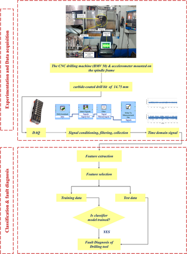
The current study used a machine-learning approach to diagnose drilling tool faults. The tool fault was diagnosed in different wear stages of drilling. The fault of the drilling tool was classified using the best first-tree algorithm. The methodology followed in the present research work is shown in Figure 6.

Key contributions of this paper are:

Data-Driven Fault Diagnosis: Implementation of a data-driven methodology for diagnosing faults in drilling tools using vibration signal analysis.
Real-Time Monitoring: Use of real-time vibration data captured through piezoelectric accelerometers under various tool wear conditions.
High Classification Accuracy: Application of the best-first tree classifier achieved a high classification accuracy of 96.2264%, demonstrating the effectiveness of the proposed method.
Practical CNC Integration: Fault diagnosis was conducted using a CNC drilling machine, making the approach directly applicable to industrial settings.
Enhanced Predictive Maintenance: The proposed system supports predictive maintenance by enabling early detection of tool wear or failure, reducing downtime and increasing operational efficiency.
Scalable and Non-Invasive: The methodology is non-invasive and can be scaled across different types of drilling operations in smart manufacturing environments.

6.2 Experimental Setup

The CNC drilling machine (BMV 50), shown in Figure 7, was used for the experiment. A piezoelectric accelerometer was used to record vibration signals during the experiment. The vibration signals were recorded during various wear phases of the drilling tool. A mild steel block was drilled during the experiments. A carbide-coated drill bit was used in the experiment. The overall length of the drill bit was 11.5 cm, and the flute length was 7.4 cm. The diameter of the present drill tool was 14.75 mm. The spindle speed and feed rate for drilling the mild steel block were 800 rpm and 71 mm/min, respectively. The depth of the cut was through a hole in a mild steel block. A Fast Fourier Transform (FFT) analyzer was used for data collection. The vibrational data acquired from the piezoelectric accelerometer were analyzed using an FFT analyzer. Figure 6 shows the workflow diagram for processing signals acquired from the data acquisition system to extract meaningful information and identify wear-related features. The next step involves model planning, where the most relevant features from the vibration data are selected, and patterns in tool wear are analyzed before applying a suitable machine learning algorithm. After identifying the predominant features affecting tool wear, data modeling uses a machine learning-based, data-driven approach to predict tool wear conditions. Finally, the model is trained and evaluated for real-time tool wear detection.

Justification for using vibration signals: The literature review identified vibration signals—especially those measured via piezoelectric accelerometers—as a reliable indicator of tool wear progression due to their sensitivity and ease of integration (see Section 3.2 of the review). This informed the choice to focus on vibration data in the experimental design.
Rationale for machine learning approach: Prior research demonstrated the high predictive accuracy of machine learning models like SVM, ANN, and decision trees for classifying tool wear stages (see Table 8 in the review). The Best First Tree algorithm was selected for its interpretability and efficiency, making it suitable for real-time deployment and comparative benchmarking.
Use of statistical feature extraction: The statistical features (mean, skewness, standard deviation, etc.) used in the experiment were directly aligned with those frequently cited in the literature as informative inputs for ML classifiers. The feature selection using the Random Tree algorithm was based on best practices to improve model generalizability and reduce dimensionality.
Experimental design alignment: The staged wear conditions (initial, slight, moderate, and severe) were designed to mirror the wear classification schemes commonly used in the reviewed studies, ensuring consistency with standard evaluation protocols.

6.3 Tool Faults Considered

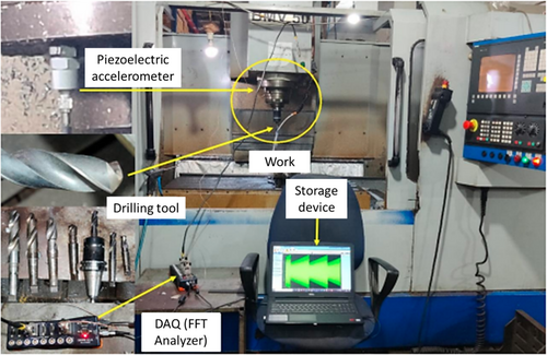
Figure 7 shows the experimental setup made for performing the drilling operation. In the first condition, experiments were performed. That is, the drilling operation was performed under the initial wear condition. Under these conditions, no wear was observed in the drilling tool. The second experiment was performed under a slight wear condition. Under this condition, very little wear was present in the tool. In the third experiment, readings were obtained with moderate wear of the drill tool, which was greater than that in the previous wear condition. In the fourth reading, the experiment was carried out under severe wear conditions, which were high compared to other drilling tool conditions. Vibration was obtained by the presence of wear in the drill tool.

6.4 Time Domain Signals

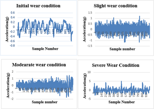
The acceleration versus sample number graph was plotted for each condition of the drill tool, as shown in Figure 8. In the initial wear conditions, the vibrations were very low; that is, they did not affect the drilling of mild steel blocks. The vibration was higher in the second condition than in the initial wear condition. In moderate wear conditions, vibrations are greater compared with both conditions, that is, initial wear and slight wear. In the last severe wear condition, vibration was more significant than in all other conditions, that is, initial, slight, and moderate wear. As wear increases in the drilling tool, the vibration increases, which can be understood from the acceleration versus sample number graph.

6.5 Statistical Feature Extraction and Best Feature Selection

6.5.1 Feature Extraction

The vibration signals obtained throughout the various wear stages of the drilling tool were acquired using a feature extraction technique. In this study, statistical features were extracted. The statistical features are mean, kurtosis, median, standard error, standard deviation, range, maximum, mode, variance, minimum, sum, count, and skewness [19, 20]. The primary visual basic code was applied to obtain all statistical features.

6.5.2 Feature Selection

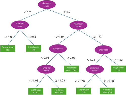
The best statistical features were selected using the random tree algorithm decision tree, as shown in Figure 9. There are 13 statistical features, and the decision tree removes seven unwanted features, namely Range, Sum, Count, Kurtosis, Median, Mode, and Mean. The decision tree selects the six best statistical features: standard error, Skewness, Maximum, Minimum, Variance, and Standard deviation. These are the six best statistical features used as inputs to the first-best algorithm.

6.5.3 Pseudocode for Best-First Tree Classifier

The pseudocode presented in Algorithm 1 formalizes the Best-First Search procedure used for feature selection or node expansion. This algorithm operates by maintaining a priority queue of candidate nodes or feature subsets, where each is evaluated using a heuristic function ℰ(S). Starting from an empty set, the algorithm iteratively selects the subset with the best evaluation score, expands it by adding one feature at a time, and updates the queue accordingly. At each step, it records the best-performing subset found so far. The process continues until all promising subsets have been explored or a stopping criterion is met. This search strategy balances greedy exploration with informed guidance from the evaluation function, making it effective for navigating high-dimensional feature spaces or tree-based decision paths.

ALGORITHM 1. Random Tree Algorithm: Decision Tree.

Inputs

𝔇 = {(x⁽ⁱ⁾, y⁽ⁱ⁾)} for i = 1 to N: Dataset with N observations

ℱ = {f₁, f₂, …, f_m}: Set of m features

ℂ = {c₁, c₂, …, c_k}: Class labels (k = 4)

ℰ(S): Evaluation function for feature subset or node S

Queue ← Priority queue ordered by ℰ(S)

S_best ← ø: Best subset or node found so far

Initialize

Queue ← {ø} (Start with empty subset)

Main Loop

while Queue ≠ ø do

S ← argmin_t ∈ Queue ℰ(T)

Queue ← Queue∖{S}

if ℰ(S) < ℰ(S_best) then

S_best ← S

for each f ∈ ℱ∖S do

S′ ← S ∪ {f}

Queue ← Queue ∪ {S′}

end while

Return

S_best (Optimal feature subset or node)

6.5.4 Hyperparameters

To guide the behavior and efficiency of the Best-First Search algorithm in feature selection, a set of key hyperparameters must be defined. Table 9 outlines these hyperparameters along with their descriptions and typical values. The evaluation metric f(n) determines the heuristic guiding the search, commonly based on Gini Index, Information Gain, or Entropy. The parameters max_nodes and max_depth constrain the search space to prevent overfitting and reduce computational cost. stopping_threshold specifies the minimum improvement required to continue exploring new nodes, acting as a convergence criterion. The search_direction controls whether features are added or removed during the search process, with forward selection being the more widely used approach. Finally, in cases of equal heuristic scores, the tie_breaker policy resolves ambiguity to maintain consistent exploration. These hyperparameters collectively balance the trade-off between search optimality and computational efficiency.

TABLE 9. Hyperparameters used while training best-first tree classifier.

Hyperparameter	Description	Values chosen
f(n)	Evaluation metric (heuristic)	Gini
max_nodes	Max nodes to explore	< 10
max_depth	Max depth of the search tree	< 5
stopping_threshold	Minimum gain improvement required	0.01
search_direction	Forward (add features) or backward (remove features)	Forward
tie_breaker	Method to break ties in score	Random

6.5.5 Results and Discussion

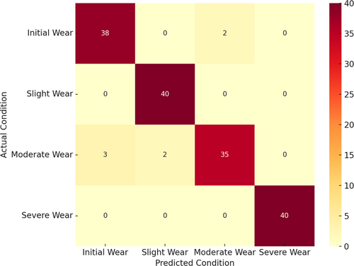
The experiment was conducted using a CNC drilling machine, and vibrational signals were acquired at different wear stages of the drilling tool. Thirteen statistical features were extracted, and the best features were chosen using a random tree algorithm decision tree, with the best first tree algorithm used to categorize the drilling tool fault. Figure 10 shows the confusion matrix for the best first tree algorithm. In total, 160 instances were used in this analysis, and 40 instances were used for each tool condition. Two cases of drilling tools with moderate wear conditions were incorrectly classified out of the 38 occurrences in which the initial wear state was correctly identified. None of the 40 occurrences in the Slight Wear condition were classified incorrectly. Thirty-five cases of moderate wear were classified appropriately. Three cases were misclassified as having initial wear under this condition, while two were misclassified as having slight wear. Finally, under severe wear conditions, all 40 instances were correctly classified; hence, there were no misclassified instances. The number of correctly classified instances in the present study was 153, and seven were classified incorrectly. The classification accuracy of correctly classified instances was 96.2264%, and that of incorrectly classified instances was 3.77365%. 5.03145% and 31.7214% represent the relative absolute error and root relative squared error, respectively. Table 10 displays the kappa statistics, mean absolute error, and relative absolute error, which were 0.9497, 0.0189, and 0.1374, respectively.

TABLE 10. Summary of the results for the best first tree algorithm.

Correctly classified instances	153	93.5%
Incorrectly classified instances	7	6.5%
Kappa statistic	0.9497
Mean absolute error	0.0189
Root mean square error	0.1374
Relative absolute error	5.0314%
Root relative squared error	31.7214%
Total number of instances	160

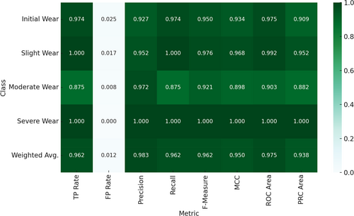
Figure 11 lists the classification accuracy in detail. The false positive (FP) and true positive (TP) rates should be close to zero and one, respectively. In this result, for all conditions of the drill tool, the TP rate is near, and the FP rate is near; hence, the model is trained correctly. The other parameters should be near 1, and from this table, it can be understood that all values are near 1 for all conditions; hence, the model is trained correctly. The TP rates were 0.974, 1.000, 0.875, and 1.000 for various drilling tool conditions, such as initial, slight, moderate, and severe. Comparably, the FP rates for the initial wear, slight wear, moderate wear, and severe wear conditions are 0.025, 0.017, 0.008, and 0.000, respectively. The results were validated using the above table considering precision, recall, F-measure, and so forth.

6.5.6 Practical Implications

Real-World Applicability: Our experiments were conducted on a CNC drilling machine under both new and worn tool conditions, closely simulating real industrial environments. This ensures that the proposed method is not only theoretically sound but also practically deployable in actual shop-floor scenarios.
Non-Invasive and Scalable Monitoring Solution: By using piezoelectric accelerometers for vibration signal acquisition, the system remains non-intrusive and cost-effective—key requirements for integration in existing manufacturing lines without the need for significant infrastructural changes.
Predictive Maintenance Enablement: The integration of machine learning enables early detection of tool wear or failure, which is vital for implementing predictive maintenance strategies. This directly translates to reduced machine downtime, lower operational costs, and prolonged tool life—critical parameters for improving overall plant productivity.
Scalability for Smart Manufacturing: The methodology lays a foundation for intelligent manufacturing systems by providing a framework that can be adapted across different machining processes and setups, facilitating the move toward Industry 4.0-ready solutions.

7 Limitations and Future Directions

The study highlights that fault characterization of drilling tool wear can aid in decision-making regarding tool life enhancement or replacement while detecting machining anomalies to improve processes and reduce operational costs. However, the vibration-based fault diagnosis approach is limited to predefined drilling parameters and may misclassify faults from unknown conditions. Future research should consider varying fault levels within each class to enhance prediction accuracy. Additionally, real-time on-board diagnosis requires diverse dataset training, which is beyond the study's scope. A deep learning-based framework is recommended, with human intervention as feedback for Reinforcement Learning (RL) to manage unforeseen faults. The proposed research can be extended to various applications:

Integration with Advanced Deep Learning Models: Exploring the use of deep learning architectures such as CNNs, LSTMs, or hybrid models for improved feature extraction and fault classification accuracy.
Multi-Sensor Data Fusion: Incorporating additional sensor data (e.g., acoustic emission, temperature, or force signals) to enhance diagnostic reliability through sensor fusion.
Real-Time Implementation on Edge Devices: Developing lightweight algorithms for real-time tool condition monitoring using embedded or edge computing devices in industrial settings.
Adaptive Diagnostic Models: Creating self-learning or adaptive models that can update themselves over time to account for new fault patterns or tool types.

8 Summary

Artificial Intelligence (AI) is increasingly applied in automated industries to enhance productivity and minimize downtime. A key strategy in achieving this is the deployment of condition-monitoring systems powered by data-driven intelligence. For effective AI-based fault diagnosis, it is essential to collect signals under varying tool conditions. In the case of drill tools, monitoring parameters such as torque, force, vibration, sound, and acoustic emissions is critical. Data acquisition is facilitated through various platforms, including FFT analyzers, NI instruments, Emerson systems, and Arduino-based setups. Signal processing techniques—such as Hilbert Transform, Hilbert-Huang Transform, time-domain, frequency-domain, and time-frequency analyses—are used to process raw sensor data. Feature extraction methods, including statistical analysis, histogram techniques, and wavelet transforms, are employed to identify key characteristics necessary for fault classification. In this study, a computer numerical control (CNC) drilling machine (BMV 50) was used to collect vibration data from the drill tool at various wear levels. Thirteen statistical features were extracted from the signal data, and the most significant features were selected using a Random Decision Tree algorithm. The Best First Tree classifier was then employed for fault categorization, achieving a classification accuracy of 96.23%. These findings demonstrate that combining statistical feature extraction with machine learning techniques enables reliable and efficient real-time fault diagnosis in drilling operations. The proposed approach is cost-effective and adaptable, making it suitable for older machine tools in small to medium-sized workshops with limited instrumentation and software resources. Future work may include sensor fusion studies and comparisons involving multiple machine learning and deep learning models across different machines.

Author Contributions

Chandan M. N: conceptualization, writing – original draft. Himadri Majumder: methodology. Sharad Mulik: data curation. Nikhil Rangaswamy: investigation, supervision. Mukesh Kumar: resources. Sowmyashree H. Srinivasaiah: writing – review and editing.

Ethics Statement

The authors have nothing to report.

Consent

The authors have nothing to report.

Conflicts of Interest

The authors declare no conflicts of interest.

Open Research

Data Availability Statement

Research data are not shared.

References

1T. I. El-Wardany, D. Gao, and M. A. Elbestawi, “Tool Condition Monitoring in Drilling Using Vibration Signature Analysis,” International Journal of Machine Tools and Manufacture 36, no. 6 (1996): 687–711.
10.1016/0890-6955(95)00058-5
Google Scholar
2G. Dheeraj Simon and R. Deivanathan, “Early Detection of Drilling Tool Wear by Vibration Data Acquisition and Classification,” Manufacturing Letters 21 (2019): 60–65, https://doi.org/10.1016/j.mfglet.2019.08.006.
10.1016/j.mfglet.2019.08.006
Google Scholar
3J. García-Sanz-Calcedo, D. R. Salgado, and A. G. González, “Drilling Projects by Tool Condition Monitoring System (TCMS),” Engineering Transactions 64, no. 4 (2016): 555–561.
Google Scholar
4M. Mikloš, J. Holubják, M. Drbúl, I. Daniš, T. Czánová, and J. Pilc, “Identification of Tool Wear When Drilling Process of Bearing Steels C56E2 With Microstructure of Lamellar Pearlite,” Transportation Research Procedia 40 (2019): 381–388, https://doi.org/10.1016/j.trpro.2019.07.056.
10.1016/j.trpro.2019.07.056
Google Scholar
5G. O'Donnell, P. Young, K. Kelly, and G. Byrne, “Towards the Improvement of Tool Condition Monitoring Systems in the Manufacturing Environment,” Journal of Materials Processing Technology 119, no. 1–3 (2001): 133–139, https://doi.org/10.1016/S0924-0136(01)00928-1.
10.1016/S0924-0136(01)00928-1
Web of Science® Google Scholar
6U. Natarajan, P. Arun, and V. M. Periasamy, “Decision Fusion Algorithm for Tool Condition Monitoring in Drilling Using Hidden Markov Model (HMM),” Indian Journal of Engineering and Materials Science 13, no. 2 (2006): 103–109.
Web of Science® Google Scholar
7M. J. Raghavendra, C. G. Ramachandra, T. R. Srinivas, and P. Pai, “Review on Tool Flank Wear Monitoring by Tool Condition Monitoring System Using Various Approaches,” GRD Journals: Global Research and Development Journals of Engineering 1, no. 4 (2016): 7–13.
Google Scholar
8R. S. Nakandhrakumar, D. Dinakaran, P. Picton, and J. Pattabiraman, “Mathematical Models of Flank Wear Using Vibration Amplitude Ratio in Drilling,” FME Transactions 47, no. 3 (2019): 430–436, https://doi.org/10.5937/fmet1903430N.
10.5937/fmet1903430N
Google Scholar
9D. E. Dimla, P. M. Lister, and N. J. Leighton, “Neural Network Solutions to the Tool Condition Monitoring Problem in Metal Cutting—A Critical Review of Methods,” International Journal of Machine Tools & Manufacture 37, no. 9 (1997): 1219–1241, https://doi.org/10.1016/S0890-6955(97)00020-5.
10.1016/S0890-6955(97)00020-5
Web of Science® Google Scholar
10P. N. Botsaris and J. A. Tsanakas, “ State-of-the-Art in Methods Applied to Tool Condition Monitoring (TCM) in Unmanned Machining Operations: A Review,” in Int. Conf. COMADEM (IEEE, 2008), 73–87.
Google Scholar
11S. Dimla and E. Dimla, “Sensor Signals for Tool-Wear Monitoring in Metal Cutting Operations: A Review of Methods,” International Journal of Machine Tools & Manufacture 40, no. 8 (2000): 1073–1098, https://doi.org/10.1016/S0890-6955(99)00122-4.
10.1016/S0890-6955(99)00122-4
Web of Science® Google Scholar
12G. Serin, B. Sener, A. M. Ozbayoglu, and H. O. Unver, “Review of Tool Condition Monitoring in Machining and Opportunities for Deep Learning,” International Journal of Advanced Manufacturing Technology 109, no. 3 (2020): 953–974.
10.1007/s00170-020-05449-w
Web of Science® Google Scholar
13N. Hu, Z. Liu, S. Jiang, et al., “Remaining Useful Life Prediction of Milling Tool Based on Pyramid CNN,” Shock and Vibration 1 (2023): 1830694.
Google Scholar
14A. G. Rehorn, J. Jiang, and P. E. Orban, “State-of-the-Art Methods and Results in Tool Condition Monitoring: A Review,” International Journal of Advanced Manufacturing Technology 26, no. 7–8 (2005): 693–710, https://doi.org/10.1007/s00170-004-2038-2.
10.1007/s00170-004-2038-2
Web of Science® Google Scholar
15A. Duo, R. Basagoiti, P. J. Arrazola, et al., “The Capacity of Statistical Features Extracted From Multiple Signals to Predict Tool Wear in the Drilling Process,” International Journal of Advanced Manufacturing Technology 102, no. 5–8 (2019): 2133–2146, https://doi.org/10.1007/s00170-019-03300-5.
10.1007/s00170-019-03300-5
Web of Science® Google Scholar
16R. Ramzi, E. A. Bakar, and M. F. Mahmod, “ Drill Bit Flank Wear Monitoring System in Composite Drilling Process Using Image Processing,” in International Conference on Robotics, Vision, Signal Processing and Power Applications (Springer Singapore, 2019), https://doi.org/10.1007/978-981-13-6447-1.
10.1007/978-981-13-6447-1_70
Google Scholar
17S. Swain, I. Panigrahi, A. K. Sahoo, and A. Panda, “Adaptive Tool Condition Monitoring System: A Brief Review,” Materials Today Proceedings 23 (2020): 474–478, https://doi.org/10.1016/j.matpr.2019.05.386.
10.1016/j.matpr.2019.05.386
Google Scholar
18A. A. Jaber and R. Bicker, “State of the Art in Research Into the Condition Monitoring of Industrial Machinery,” International Journal of Current Engineering and Technology 4, no. 3 (2014): 1986–2001.
Google Scholar
19A. Przybyś-Małaczek, I. Antoniuk, K. Szymanowski, M. Kruk, and J. Kurek, “Application of Machine Learning Algorithms for Tool Condition Monitoring in Milling Chipboard Process,” Sensors 23, no. 13 (2023): 5850.
10.3390/s23135850
Web of Science® Google Scholar
20C. Zhang, X. Yao, J. Zhang, and H. Jin, “Tool Condition Monitoring and Remaining Useful Life Prognostic Based on a Wireless Sensor in Dry Milling Operations,” Sensors 16, no. 6 (2016): 795.
10.3390/s16060795
Web of Science® Google Scholar
21M. Amarnath, P. Ramakrishna, and H. Challadurai, “Detection of Tool Wear in Drilling Process Using Vibration Signal Analysis,” International Journal of Mechanical And Production Engineering 5, no. 29 (2017): 136–138.
Google Scholar
22E. Jantunen, “Summary of Methods Applied to Tool-Condition Monitoring During Drilling,” International Journal of Machine Tools & Manufacture 42, no. 9 (2002): 997–1010, https://doi.org/10.1016/S0890-6955(02)00040-8.
10.1016/S0890-6955(02)00040-8
Google Scholar
23S. Dutta, S. K. Pal, S. Mukhopadhyay, and R. Sen, “Application of Digital Image Processing in Tool Condition Monitoring: A Review,” CIRP Journal of Manufacturing Science and Technology 6, no. 3 (2013): 212–232, https://doi.org/10.1016/j.cirpj.2013.02.005.
10.1016/j.cirpj.2013.02.005
Google Scholar
24Q. Zhang, D. Zhao, and D. Wang, “ Event-Triggered Adaptive Dynamic Programming for Uncertain Nonlinear Systems,” in Cognitive Systems and Signal Processing (Springer, 2017), 13–26, https://doi.org/10.1007/978-981-10-5230-9_2.
10.1007/978-981-10-5230-9_2
Google Scholar
25S. Hu, D. Yue, X. Yin, X. Xie, and Y. Ma, “Adaptive Event-Triggered Control for Nonlinear Discrete-Time Systems,” International Journal of Robust and Nonlinear Control 26, no. 18 (2016): 4104–4125, https://doi.org/10.1002/rnc.3550.
10.1002/rnc.3550
Web of Science® Google Scholar
26L. Chu and Y. Liu, “Adaptive Event-Triggered Control for Nonlinear Systems With Time-Varying Parameter Uncertainties,” International Journal of Robust and Nonlinear Control 34, no. 3 (2023): 2094–2108, https://doi.org/10.1002/rnc.7072.
10.1002/rnc.7072
Web of Science® Google Scholar
27Y. Liu, G. Qiu, W. Gou, and Q. Liu, “Event-Triggered Adaptive Dynamic Programming of Nonlinear System With Asymmetric Input Constraints and Uncertain Disturbances,” Optimal Control Applications and Methods 44, no. 5 (2023): 2281–2297, https://doi.org/10.1002/oca.2977.
10.1002/oca.2977
Web of Science® Google Scholar
28Y. Zhao, X. Dai, D. Gong, X. Lv, and Y. Liu, “Event-Triggered Adaptive Dynamic Programming Consensus Tracking Control for Discrete-Time Multiagent Systems,” Complexity 2022 (2022): 6028054, https://doi.org/10.1155/2022/6028054.
10.1155/2022/6028054
Web of Science® Google Scholar
29Y. Liang, J. Zhang, H. Zhao, H. Su, and X. Cui, “A Learning-Based Approach to Event-Triggered Guaranteed Cost Control for Completely Unknown Nonlinear Systems,” Transactions of the Institute of Measurement and Control 46, no. 1 (2024): 3–15, https://doi.org/10.1177/01423312231185383.
10.1177/01423312231185383
Google Scholar
30Z. Peng, Z. Zhang, R. Luo, Y. Kuang, J. Hu, and H. Cheng, “Event-Triggered Optimal Control of Completely Unknown Nonlinear Systems via Identifier-Critic Learning,” Kybernetika 59, no. 3 (2023): 365–391.
Web of Science® Google Scholar
31U. Siddique, A. Sinha, and Y. Cao, “Adaptive Event-Triggered Reinforcement Learning Control for Complex Nonlinear Systems,” arXiv Preprint arXiv:2409.19769, 2024, https://arxiv.org/abs/2409.19769.
Google Scholar
32T. Radhakrishnan and S. M. Wu, “Online Hole Quality Evaluation for Drilling Composite Material Using Dynamic Data,” American Society of Mechanical Engineers 103, no. 1 (1980): 119–125.
Google Scholar
33M. Routio and M. Säynätjoki, “Tool Wear, and Failure in the Drilling of Stainless Steel,” Journal of Materials Processing Technology 52, no. 1 (1995): 35–43, https://doi.org/10.1016/0924-0136(94)01441-3.
10.1016/0924-0136(94)01441-3
Web of Science® Google Scholar
34K. Subramanian and N. H. Cook, “Sensing of Drill Wear and Prediction of Drill Life,” Journal of Manufacturing Science and Engineering. Transactions of the ASME 99, no. 2 (1977): 295–301, https://doi.org/10.1115/1.3439211.
10.1115/1.3439211
Google Scholar
35A. Noori-Khajavi, Frequency and Time Domain Analyses of Sensor Signals in a Drilling Process and Their Coordination With Drill Wear (Mechanical Engineering, Oklahoma State University, 1992), 1–207.
Google Scholar
36A. Noori-Khajavi and R. Komanduri, “On Multisensor Approach to Drill Wear Monitoring,” CIRP Annals—Manufacturing Technology 42, no. 1 (1993): 71–74, https://doi.org/10.1016/S0007-8506(07)62394-4.
10.1016/S0007-8506(07)62394-4
Google Scholar
37K. Ramamurthi and C. Hough, “Intelligent Real-Time Predictive Diagnostics for Cutting Tools and Supervisory Control of Machining Operations,” Journal of Manufacturing Science and Engineering. Transactions of the ASME 115, no. 3 (1993): 268–277, https://doi.org/10.1115/1.2901660.
10.1115/1.2901660
Google Scholar
38M. Valikhani and S. Chandrashekhar, “An Experimental Investigation Into the Comparison of the Performance Characteristics of TiN and ZrN Coatings on Split Point Drills Using the Static and Stochastic Models of the Force System as a Signature,” International Journal of Advanced Manufacturing Technology 2, no. 1 (1987): 75–106, https://doi.org/10.1007/BF02601470.
10.1007/BF02601470
Google Scholar
39E. Brinksmeier, “Prediction of Tool Fracture in Drilling,” CIRP Annals—Manufacturing Technology 39, no. 1 (1990): 97–100, https://doi.org/10.1016/S0007-8506(07)61011-7.
10.1016/S0007-8506(07)61011-7
Google Scholar
40G. S. Li, W. S. Lau, and Y. Z. Zhang, “In-Process Drill Wear and Breakage Monitoring for a Machining Center Based on Cutting Force Parameters,” International Journal of Machine Tools & Manufacture 32, no. 6 (1992): 855–867, https://doi.org/10.1016/0890-6955(92)90035-F.
10.1016/0890-6955(92)90035-F
Web of Science® Google Scholar
41A. Noori-Khajavi and R. Komanduri, “Frequency and Time-Domain Analyses of Sensor Signals in Drilling-I. Correlation With Drill Wear,” International Journal of Machine Tools & Manufacture 35, no. 6 (1995): 775–793, https://doi.org/10.1016/0890-6955(94)00060-W.
10.1016/0890-6955(94)00060-W
Google Scholar
42H. M. Ertunc, K. A. Loparo, and H. Ocak, “Tool Wear Condition Monitoring in Drilling Operations Using Hidden Markov Models (HMMs),” International Journal of Machine Tools and Manufacture 41, no. 9 (2001): 1363–1384, https://doi.org/10.1016/S0890-6955(00)00112-7.
10.1016/S0890-6955(00)00112-7
Web of Science® Google Scholar
43O. Yumak and H. M. Ertunc, “Tool Wear Condition Monitoring in Drilling Processes Using Fuzzy Logic,” Lecture Notes in Computer Science 4234 (2006): 508–517.
10.1007/11893295_56
Web of Science® Google Scholar
44S. S. Panda, D. Chakraborty, and S. K. Pal, “Monitoring of Drill Flank Wear Using Fuzzy Back-Propagation Neural Network,” International Journal of Advanced Manufacturing Technology 34, no. 3–4 (2007): 227–235, https://doi.org/10.1007/s00170-006-0589-0.
10.1007/s00170-006-0589-0
Web of Science® Google Scholar
45R. Vimal Sam Singh, B. Latha, and V. S. Senthilkumar, “Modeling and Analysis of Thrust Force and Torque in Drilling GFRP Composites by Multi-Facet Drill Using Fuzzy Logic,” International Journal of Current Trends in Engineering and Technology 1, no. 5 (2009): 66–70.
Google Scholar
46J. Yu, “Online Tool Wear Prediction in Drilling Operations Using Selective Artificial Neural Network Ensemble Model,” Neural Computing & Applications 20, no. 4 (2011): 473–485, https://doi.org/10.1007/s00521-011-0539-0.
10.1007/s00521-011-0539-0
Web of Science® Google Scholar
47R. Corne, C. Nath, M. El Mansori, and T. Kurfess, “Study of Spindle Power Data With Neural Network for Predicting Real-Time Tool Wear/Breakage During Inconel Drilling,” Journal of Manufacturing Systems 43 (2017): 287–295, https://doi.org/10.1016/j.jmsy.2017.01.004.
10.1016/j.jmsy.2017.01.004
Web of Science® Google Scholar
48A. Caggiano, P. Centobelli, L. Nele, and R. Teti, “Multiple Sensor Monitoring in Drilling of CFRP/CFRP Stacks for Cognitive Tool Wear Prediction and Product Quality Assessment,” Procedia CIRP 62 (2017): 3–8, https://doi.org/10.1016/j.procir.2017.03.047.
10.1016/j.procir.2017.03.047
Google Scholar
49L. H. Saw, L. W. Ho, M. C. Yew, et al., “Sensitivity Analysis of Drill Wear and Optimization Using Adaptive Neuro-Fuzzy–Genetic Algorithm Technique Toward Sustainable Machining,” Journal of Cleaner Production 172 (2018): 3289–3298, https://doi.org/10.1016/j.jclepro.2017.10.303.
10.1016/j.jclepro.2017.10.303
Web of Science® Google Scholar
50R. Teti, T. Segreto, and A. Caggiano, “Smart Multisensor Monitoring in Drilling of CFRP/CFRP Composite Material Stacks for Aerospace Assembly Applications,” Applied Sciences 10, no. 3 (2020): 758, https://doi.org/10.3390/app10030758.
10.3390/app10030758
CAS Google Scholar
51M. A. Alcon, L. N. López de Lacalle, and F. F. Zacarías, “Multiple Sensor Monitoring of CFRP Drilling to Define Cutting Parameter Sensitivity on Surface Roughness, Cylindricity, and Diameter,” Materials, MPDI 13, no. 12 (2020): 1–17.
Google Scholar
52T. Barik, S. K. Jena, S. Gahir, K. Pal, and S. K. Pattnaik, “Materials Today: Proceedings Process Parametric Optimization in Drilling of CFRP Composites Using GRA Method,” Materials Today Proceedings 39 (2020): 1281–1286, https://doi.org/10.1016/j.matpr.2020.04.220.
10.1016/j.matpr.2020.04.220
Google Scholar
53A. Padro, R. Heinemann, N. M. Nobre, and L. Bagshaw, “Assessment of Decision-Making Algorithms for Adaptive Drilling of Aerospace Stack,” Procedia CIRP 99 (2020): 392–397, https://doi.org/10.1016/j.procir.2021.03.055.
10.1016/j.procir.2021.03.055
Google Scholar
54G. Zhu, S. Hu, and H. Tang, “Prediction of Tool Wear in CFRP Drilling Based on a Neural Network With Multi-Characteristics and Multi-Signal Sources,” Composites. Part A, Applied Science and Manufacturing 30 (2021): 2633366X2098723, https://doi.org/10.1177/2633366x20987234.
10.1177/2633366x20987234
Google Scholar
55M. Senthilkumar, A. Prabukarthi, and V. Krishnaraj, “Machining of CFRP/Ti6Al4V Stacks Under Minimal Quantity Lubrication Condition,” Journal of Mechanical Science and Technology 32, no. 8 (2018): 3787–3796, https://doi.org/10.1007/s12206-018-0731-6.
10.1007/s12206-018-0731-6
Google Scholar
56V. Karri and T. Kiatcharoenpol, “Tool Condition Monitoring in Drilling Using Artificial Neural Networks,” Lecture Notes in Computer Science 2903, no. 91 (2003): 293–301, https://doi.org/10.1117/12.380593.
10.1007/978-3-540-24581-0_25
Google Scholar
57Y. Shi, H. Liu, X. Zhang, Q. Li, and X. Guo, “Wear Identification of Vibration Drilling Bit Based on Improved LMD and BP Neural Networks,” Mathematical Problems in Engineering 2020 (2020): 1–9.
Google Scholar
58P. K. Kumar and P. Kuppan, “Online Monitoring of Delamination Mechanisms in Drilling of Wcnts Reinforced Gfrp Nanocomposites by Acoustic Emission,” Materials Today Proceedings 5, no. 5 (2018): 13036–13047, https://doi.org/10.1016/j.matpr.2018.02.290.
10.1016/j.matpr.2018.02.290
CAS Google Scholar
59N. Chen, B. Hao, Y. Guo, L. Li, M. A. Khan, and N. He, “Research on Tool Wear Monitoring in Drilling Process Based on APSO-LS-SVM Approach, Approach,” International Journal of Advanced Manufacturing Technology 108 (2020): 2091–2101.
10.1007/s00170-020-05549-7
Google Scholar
60I. Kandilli, M. Sönmez, H. M. Ertunc, and B. Çakir, “ Online Monitoring of Tool Wear in Drilling and Milling by Multisensor Neural Network Fusion,” in Proc. 2007 IEEE Int. Conf. Mechatronics Autom 2007 (ICMA, 2007), 1388–1394, https://doi.org/10.1109/ICMA.2007.4303752.
Google Scholar
61A. Duo, R. Basagoiti, P. J. Arrazola, T. Segreto, R. Teti, and A. Caggiano, “Drilling Process Monitoring: A Framework for Data Gathering and Feature Extraction Techniques,” Procedia CIRP 99 (2021): 189–195, https://doi.org/10.1016/j.procir.2021.03.123.
10.1016/j.procir.2021.03.123
Google Scholar
62A. Jegorowa, J. Górski, J. Kurek, and M. Kruk, “Initial Study on the Use of Support Vector Machine (SVM) in Tool Condition Monitoring in Chipboard Drilling,” European Journal of Wood and Wood Products 77, no. 5 (2019): 957–959, https://doi.org/10.1007/s00107-019-01428-5.
10.1007/s00107-019-01428-5
CAS Web of Science® Google Scholar
63K. Ranjan, T. Patra, M. Szalay, et al., “Pimenov, Artificial-Intelligence-Based Hole-Quality Prediction,” Sensors 20, no. 3 (2020): 1–14.
Google Scholar
64P. S. Heyns, “Tool Condition Monitoring Using Vibration Measurements—A Review,” OR Insight 49, no. 8 (2007): 447–450, https://doi.org/10.1784/insi.2007.49.8.447.
10.1784/insi.2007.49.8.447
Google Scholar
65R. W. Barker, G. Klutke, and M. J. Hinich, “Monitoring Rotating Tool Wear Using Higher-Order Spectral Features,” Journal of Manufacturing Science and Engineering. Transactions of the ASME 115, no. 1 (1993): 23–29, https://doi.org/10.1115/1.2901634.
10.1115/1.2901634
Google Scholar
66T. I. Liu and S. M. Wu, “Online Detection of Drill Wear,” Journal of Engineering 112, no. August (1990): 299–302.
Google Scholar
67J. Yan and J. Lee, “ Hybrid Method for Online Performance Assessment and Life Prediction in Drilling Operations,” in Proc. IEEE Int. Conf. Autom. Logist. ICAL 2007 (IEEE, 2007), 2500–2505, https://doi.org/10.1109/ICAL.2007.4338999.
Google Scholar
68R. S. Nakandhrakumar, D. Dinakaran, M. Gopal, and J. Pattabiraman, “Novel Normalization Procedure for the Sensor Positioning Problem in Vibration Monitoring of Drilling Using Artificial Neural Networks,” Insight – Non-Destructive Testing and Condition Monitoring 58, no. 10 (2016): 556–563, https://doi.org/10.1784/insi.2016.58.10.556.
10.1784/insi.2016.58.10.556
Google Scholar
69A. Kumar, J. Ramkumar, N. K. Verma, and S. Dixit, “ Detection and Classification for Faults in Drilling Process Using Vibration Analysis,” in 2014 Int. Conf. Progn. Heal. Manag. PHM 2014 (ICPHM, 2015), 3–8, https://doi.org/10.1109/ICPHM.2014.7036393.
Google Scholar
70N. Arunkumar, A. Thanikasalam, V. Sankaranarayanan, and E. Senthilkumar, “Parametric Optimization of Deep-Hole Drilling on AISI 1045 Steel and Online Tool Condition Monitoring Using an Accelerometer,” Materials and Manufacturing Processes 33, no. 16 (2018): 1751–1764, https://doi.org/10.1080/10426914.2018.1476757.
10.1080/10426914.2018.1476757
CAS Web of Science® Google Scholar
71B. S. Prasad and D. S. Sai Ravi Kiran, “Experimental Investigation to Optimize Tool Performance in High-Speed Drilling: A Comparative Study,” Journal of the Brazilian Society of Mechanical Sciences and Engineering 41, no. 11 (2019): 535, https://doi.org/10.1007/s40430-019-2049-4.
10.1007/s40430-019-2049-4
Web of Science® Google Scholar
72R. John Stephen, T. Thangeswari, S. Palani, and D. Dinakaran, “Condition Monitoring in Drilling Operation Based on Vibration Signals,” International Journal of Recent Technology and Engineering 8, no. 3 (2019): 1272–1277, https://doi.org/10.35940/ijrte.C4416.098319.
10.35940/ijrte.C4416.098319
Google Scholar
73C. N. Hsu, Y. C. Lin, C. C. Yang, et al., “ Low-Cost Vibration and Acceleration Sensors Module for the Drilling Processes Monitoring,” in SAS 2019–2019 IEEE Sensors Appl. Symp. Conf. Proc (IEEE, 2019), 1–5, https://doi.org/10.1109/SAS.2019.8705991.
Google Scholar
74R. Singhal, A. Kumar, S. Zafar, and V. Dutt, “ Evaluating Statistical Approaches for Tool Condition Monitoring in Drilling Applications,” in Lecture Notes on Multidisciplinary Industrial Engineering Optimization Methods in Engineering, ed. J. P. Davim (Springer, 2019).
Google Scholar
75S. R. Hayashi, C. E. Thomas, D. G. Wildes, and G. Tlusty, “Tool Break Detection by Monitoring Ultrasonic Vibrations,” CIRP Annals – Manufacturing Technology 37, no. 1 (1988): 61–64, https://doi.org/10.1016/S0007-8506(07)61586-8.
10.1016/S0007-8506(07)61586-8
Google Scholar
76A. L. Quadro and J. R. T. Branco, “Analysis of the Acoustic Emission During Drilling Test,” Surface and Coatings Technology 94–95, no. 1997 (1997): 691–695, https://doi.org/10.1016/S0257-8972(97)00509-4.
10.1016/S0257-8972(97)00509-4
CAS Google Scholar
77T. Jessel, C. Byrne, M. Eaton, B. Merrifield, S. Harris, and R. Pullin, “Tool Condition Monitoring of Diamond-Coated Burrs With Acoustic Emission Utilising Machine Learning Methods,” International Journal of Advanced Manufacturing Technology 130, no. 3–4 (2024): 1107–1124, https://doi.org/10.1007/s00170-023-12700-7.
10.1007/s00170-023-12700-7
Web of Science® Google Scholar
78K. Thirukkumaran and C. K. Mukhopadhyay, “Analysis of Acoustic Emission Signal to Characterize the Damage Mechanism During Drilling of Al-5% SiC Metal Matrix Composite,” 2020.
Google Scholar
79X. Li, Y. Yao, and Z. Yuan, “Online Tool Condition Monitoring System With Wavelet Fuzzy Neural Network,” Journal of Intelligent Manufacturing 8, no. 4 (1997): 271–276, https://doi.org/10.1023/A:1018585527465.
10.1023/A:1018585527465
Google Scholar
80A. Velayudham, R. Krishnamurthy, and T. Soundarapandian, “Acoustic-Emission-Based Drill Condition Monitoring During Drilling of Glass/Phenolic Polymeric Composite Using Wavelet Packet Transform,” Materials Science and Engineering A 412, no. 1–2 (2005): 141–145, https://doi.org/10.1016/j.msea.2005.08.036.
10.1016/j.msea.2005.08.036
Web of Science® Google Scholar
81F. Klocke, B. Döbbeler, T. Pullen, and T. Bergs, “Acoustic Emission Signal Source Separation for a Flank Wear Estimation of Drilling Tools,” Procedia CIRP 79, no. i (2019): 57–62, https://doi.org/10.1016/j.procir.2019.02.011.
10.1016/j.procir.2019.02.011
Google Scholar
82K. Patra, “Acoustic Emission Based Tool Condition Monitoring System in Drilling,” Proceedings of the World Congress on Engineering III (2011): 5–9.
Google Scholar
83M. P. Gómez, A. M. Hey, J. E. Ruzzante, and C. E. D'Attellisc, “Tool Wear Evaluation in Drilling by Acoustic Emission,” Physics Procedia 3, no. 1 (2010): 819–825, https://doi.org/10.1016/j.phpro.2010.01.105.
10.1016/j.phpro.2010.01.105
Google Scholar
84L. R. R. Silva, V. T. S. Claro, V. T. S. Del, and C. L. F. Andrade, “Tool Wear Monitoring in Drilling of High-Strength Compacted Graphite Cast Iron,” Journal of Engineering Manufacture 235, no. 1–2 (2020): 207–218, https://doi.org/10.1177/0954405420937857.
10.1177/0954405420937857
Google Scholar
85S. Leng, Z. Wang, T. Min, Z. Dai, and G. Chen, “Detection of Tool Wear in Drilling CFRP/TC4 Stacks by Acoustic Emission,” Journal of Vibration Engineering & Technology 8, no. June 2020 (2019): 463–470, https://doi.org/10.1007/s42417-019-00190-5.
10.1007/s42417?019?00190?5
Google Scholar
86N. Heidary, Z. Karimi, M. Karimi, A. Ahmadi, A. Rahimi, and A. Zucchelli, “Clustering of Acoustic Emission Signals Collected During Drilling Process of Composite Materials Using Unsupervised Classifiers,” Journal of Composite Materials 49, no. 5 (2014): 559–571, https://doi.org/10.1177/0021998314521258.
10.1177/0021998314521258
Google Scholar
87N. Z. Karimi, G. Minak, and P. Kianfar, “Analysis of Damage Mechanisms in Drilling of Composite Materials by Acoustic Emission,” Composite Structures 131, no. November 2015 (2015): 107–114, https://doi.org/10.1016/j.compstruct.2015.04.025.
10.1016/j.compstruct.2015.04.025
Google Scholar
88S. R. Ravishankar and C. R. L. Murthy, “Application of Acoustic Emission in Drilling of Composite Laminates,” NDT and E International 33 (2000): 429–435.
10.1016/S0963-8695(00)00014-1
Web of Science® Google Scholar
89F. Erdélyi and C. Sántha, “Monitoring Tasks on Boring and Milling Production Cells,” Computers in Industry 7, no. 1 (1986): 65–71, https://doi.org/10.1016/0166-3615(86)90010-2.
10.1016/0166-3615(86)90010-2
Web of Science® Google Scholar
90X. Li, “Online Detection of the Breakage of Small-Diameter Drills Using Current Signature Wavelet Transform,” International Journal of Machine Tools & Manufacture 39, no. 1 (1999): 157–164, https://doi.org/10.1016/s0890-6955(97)00066-7.
10.1016/S0890-6955(97)00066-7
Google Scholar
91L. A. Franco-Gasca, G. Herrera-Ruiz, R. Peniche-Vera, R. D. J. Romero-Troncoso, and W. Leal-Tafolla, “Sensorless Tool Failure Monitoring System for Drilling Machines,” International Journal of Machine Tools and Manufacture 46, no. 3–4 (2006): 381–386, https://doi.org/10.1016/j.ijmachtools.2005.05.012.
10.1016/j.ijmachtools.2005.05.012
Web of Science® Google Scholar
92X. Li, S. K. Tso, and J. Wang, “Real-Time Tool Condition Monitoring Using Wavelet Transforms and Fuzzy Techniques,” IEEE Transactions on Systems, Man, and Cybernetics, Part C, Applications and Reviews 30, no. 3 (2000): 352–357, https://doi.org/10.1109/5326.885116.
10.1109/5326.885116
Web of Science® Google Scholar
93M. Klaic, T. Staroveski, and T. Udiljak, “Tool Wear Classification Using Decision Tree Stone Drilling Applications: A Preliminary Study,” Procedia Engineering 69 (2014): 1326–1335, https://doi.org/10.1016/j.proeng.2014.03.125.
10.1016/j.proeng.2014.03.125
Google Scholar
94T. Sathish and D. Chandramohan, “Experimental Study and Model Development for Online Drill Wear Monitoring System Using Lab View,” International Journal of Recent Technology and Engineering 7, no. 6 (2019): 281–286.
Google Scholar
95U. Guide, “AMS 2140 Machinery Health Analyzer User Guide,” 2019.
Google Scholar
96G. F. Wang, Y. W. Yang, Y. C. Zhang, and Q. L. Xie, “Vibration Sensor-Based Tool Condition Monitoring Using ν Support Vector Machine and Locality Preserving Projection,” Sensors and Actuators, A: Physical 209 (2014): 24–32, https://doi.org/10.1016/j.sna.2014.01.004.
10.1016/j.sna.2014.01.004
CAS Google Scholar
97K. Patra, A. K. Jha, T. Szalay, J. Ranjan, and L. Monostori, “Artificial Neural Network Based Tool Condition Monitoring in Micro Mechanical Peck Drilling Using Thrust Force Signals,” Precision Engineering 48 (2017): 279–291, https://doi.org/10.1016/j.precisioneng.2016.12.011.
10.1016/j.precisioneng.2016.12.011
Web of Science® Google Scholar
98G. Dong Wang, N. Li, S. Melly, et al., “Monitoring the Drilling Process of GFRP Laminates With Carbon Nanotube Buckypaper Sensor,” Composite Structures 208, no. 1 (2019): 114–126, https://doi.org/10.1016/j.compstruct.2018.10.016.
10.1016/j.compstruct.2018.10.016
Google Scholar
99J. Susai Mary, S. A. Balaji, A. Krishnakumari, R. S. Nakandhrakumar, and D. Dinakaran, “Monitoring of Drill Runout Using Least Squares Support Vector Machine Classifier,” Measurement: Journal of the International Measurement Confederation 146 (2019): 24–34, https://doi.org/10.1016/j.measurement.2019.05.102.
10.1016/j.measurement.2019.05.102
Google Scholar
100N. Dhobale, S. Mulik, R. Jegadeeshwaran, and A. Patange, “Supervision of Milling Tool Inserts Using Conventional and Artificial Intelligence Approach: A Review,” Sound and Vibration 55, no. 2 (2021): 87–116, https://doi.org/10.32604/SV.2021.014224.
10.32604/SV.2021.014224
Web of Science® Google Scholar
101N. Dhobale, S. Mulik, R. Jegdeeshwaran, and K. Ganer, “Multipoint Milling Tool Supervision Using Artificial Neural Network Approach,” Materials Today Proceedings 45 (2021): 1898–1903, https://doi.org/10.1016/j.matpr.2020.09.147.
10.1016/j.matpr.2020.09.147
Google Scholar
102C. I. Noshi and J. J. Schubert, “ The Role of Machine Learning in Drilling Operations; A Review,” in SPE Eastern Regional Meeting (SPE, 2018), 7–11, https://doi.org/10.2118/191823-18erm-ms.
Google Scholar
103N. Tambake, B. Deshmukh, S. Pardeshi, S. Salunkhe, R. Čep, and E. Abouel Nasr, “Condition Monitoring of a CNC Hobbing Cutter Using Machine Learning Approach,” Advanced Mechanical Engineering 16, no. 9 (2024): 1–14, https://doi.org/10.1177/16878132241275750.
10.1177/16878132241275750
Web of Science® Google Scholar
104S. Omole, H. Dogan, A. J. G. Lunt, S. Kirk, and A. Shokrani, “Using Machine Learning for Cutting Tool Condition Monitoring and Prediction During Machining of Tungsten,” International Journal of Computer Integrated Manufacturing 37, no. 6 (2024): 747–771, https://doi.org/10.1080/0951192X.2023.2257648.
10.1080/0951192X.2023.2257648
Web of Science® Google Scholar
105C. Domínguez-Monferrer, A. Ramajo-Ballester, J. M. Armingol, and J. L. Cantero, “Spot-Checking Machine Learning Algorithms for Tool Wear Monitoring in Automatic Drilling Operations in CFRP/Ti6Al4V/Al Stacks in the Aircraft Industry,” Journal of Manufacturing Systems 77, no. April (2024): 96–111, https://doi.org/10.1016/j.jmsy.2024.08.023.
10.1016/j.jmsy.2024.08.023
Google Scholar
106D. Mishra, K. R. Pattipati, and G. M. Bollas, “Gaussian Mixture Model for Tool Condition Monitoring,” Journal of Manufacturing Processes 131, no. April (2024): 1001–1013, https://doi.org/10.1016/j.jmapro.2024.09.038.
10.1016/j.jmapro.2024.09.038
Google Scholar
107M. D. Surindra, G. A. F. Alfarisy, W. Caesarendra, et al., “Use of Machine Learning Models in Condition Monitoring of Abrasive Belt in Robotic Arm Grinding Process,” Journal of Intelligent Manufacturing 36 (2024): 3345–3358, https://doi.org/10.1007/s10845-024-02410-6.
10.1007/s10845-024-02410-6
Web of Science® Google Scholar
108M. A. Lara de Leon, J. Kolarik, R. Byrtus, J. Koziorek, P. Zmij, and R. Martinek, “Tool Condition Monitoring Methods Applicable in the Metalworking Process,” Archives of Computational Methods in Engineering 31, no. 1 (2024): 221–242, https://doi.org/10.1007/s11831-023-09979-w.
10.1007/s11831-023-09979-w
Google Scholar
109A. D. Patange and R. Jegadeeshwaran, “A Machine Learning Approach for Vibration-Based Multipoint Tool Insert Health Prediction on Vertical Machining Centre (VMC),” Measurement: Journal of the International Measurement Confederation 173, no. September 2020 (2021): 108649, https://doi.org/10.1016/j.measurement.2020.108649.
10.1016/j.measurement.2020.108649
Google Scholar
110M. Kuntoğlu and H. Sağlam, “Investigation of Signal Behaviors for Sensor Fusion With Tool Condition Monitoring System in Turning,” Measurement: Journal of the International Measurement Confederation 173, no. September 2020 (2021): 1–15, https://doi.org/10.1016/j.measurement.2020.108582.
10.1016/j.measurement.2020.108582
Google Scholar
111Y. Liang, S. Hu, W. Guo, and H. Tang, “Abrasive Tool Wear Prediction Based on an Improved Hybrid Difference Grey Wolf Algorithm for Optimizing SVM,” Measurement: Journal of the International Measurement Confederation 187, no. November 2021 (2022): 110247, https://doi.org/10.1016/j.measurement.2021.110247.
10.1016/j.measurement.2021.110247
Google Scholar
112N. S. Bajaj, A. D. Patange, R. Jegadeeshwaran, S. S. Pardeshi, K. A. Kulkarni, and R. S. Ghatpande, “Application of Metaheuristic Optimization Based Support Vector Machine for Milling Cutter Health Monitoring,” Intelligent Systems With Applications 18, no. December 2022 (2023): 200196, https://doi.org/10.1016/j.iswa.2023.200196.
10.1016/j.iswa.2023.200196
Google Scholar
113A. Nautiyal and A. K. Mishra, “Machine Learning Application in Enhancing Drilling Performance,” Procedia Computer Science 218, no. 2022 (2022): 877–886, https://doi.org/10.1016/j.procs.2023.01.068.
10.1016/j.procs.2023.01.068
Google Scholar
114A. D. Patange, R. Jegadeeshwaran, N. S. Bajaj, A. N. Khairnar, and N. A. Gavade, “Application of Machine Learning for Tool Condition Monitoring in Turning,” Sound and Vibration 56, no. 2 (2022): 127–145, https://doi.org/10.32604/sv.2022.014910.
10.32604/sv.2022.014910
Web of Science® Google Scholar
115B. Brophy, K. Kelly, and G. Byrne, “AI-Based Condition Monitoring of the Drilling Process,” Journal of Materials Processing Technology 124, no. 3 (2002): 305–310, https://doi.org/10.1016/S0924-0136(02)00201-7.
10.1016/S0924-0136(02)00201-7
Web of Science® Google Scholar
116S. Ferrisi, G. Zangara, D. R. Izquierdo, et al., “Tool Condition Monitoring for Milling Process Using Convolutional Neural Networks,” Procedia Computer Science 232, no. 2023 (2024): 1607–1616, https://doi.org/10.1016/j.procs.2024.01.158.
10.1016/j.procs.2024.01.158
Google Scholar
117T. Reeber, J. Henninger, N. Weingarz, et al., “Tool Condition Monitoring in Drilling Processes Using Anomaly Detection Approaches Based on Control Internal Data,” Procedia CIRP 121 (2024): 216–221, https://doi.org/10.1016/j.procir.2023.08.066.
10.1016/j.procir.2023.08.066
Google Scholar
118S. Ferrisi, G. Ambrogio, R. Guido, and D. Umbrello, “Artificial Intelligence Techniques and Internet of Things Sensors for Tool Condition Monitoring in Milling: A Review,” Materials Research Proceedings 41 (2024): 2000–2010, https://doi.org/10.21741/9781644903131-221.
10.21741/9781644903131-221
Google Scholar
119M. Umar, M. F. Siddique, N. Ullah, and J. M. Kim, “Milling Machine Fault Diagnosis Using Acoustic Emission and Hybrid Deep Learning With Feature Optimization,” Applied Sciences 14, no. 22 (2024): 1–22, https://doi.org/10.3390/app142210404.
10.3390/app142210404
Google Scholar
120D. Kaliyannan, M. Thangamuthu, P. Pradeep, S. Gnansekaran, J. Rakkiyannan, and A. Pramanik, “Tool Condition Monitoring in the Milling Process Using Deep Learning and Reinforcement Learning,” Journal of Sensor and Actuator Networks 13, no. 4 (2024): 42, https://doi.org/10.3390/jsan13040042.
10.3390/jsan13040042
Web of Science® Google Scholar
121D. Y. Pimenov, L. R. R. da Silva, A. Ercetin, O. Der, T. Mikolajczyk, and K. Giasin, “State-of-the-Art Review of Applications of Image Processing Techniques for Tool Condition Monitoring on Conventional Machining Processes,” International Journal of Advanced Manufacturing Technology 130, no. 1–2 (2024): 57–85, https://doi.org/10.1007/s00170-023-12679-1.
10.1007/s00170-023-12679-1
Web of Science® Google Scholar
122B. Rüstem, K. Mustafa, P. Danil Yu, A. U. Üsame, G. Munish Kumar, and K. Mehmet Erdi, “Advance Monitoring of Hole Machining Operations via Intelligent Measurement Systems: A Critical Review and Future Trends,” Measurement: Journal of the International Measurement Confederation 201, no. August (2022): 1–27, https://doi.org/10.1016/j.measurement.2022.111757.
10.1016/j.measurement.2022.111757
Google Scholar
123K. K. Powar, A. N. Kalll, M. G. Avalappa, et al., “Multi-Objective Optimization of Dry Turning of Inconel 718 Utilizing Grey Relational Analysis,” Journal of Aeronautics, Astronautics and Aviation 57, no. 2 (2025): 151–160, https://doi.org/10.6125/JoAAA.202503_57(2).02.
10.6125/JoAAA.202503_57(2).02
Web of Science® Google Scholar
124S. Paul, R. Turnbull, D. Khodadad, and M. Löfstrand, “A Vibration-Based Automatic Fault Detection Scheme for Drilling Process Using Type-2 Fuzzy Logic,” Algorithms 15, no. 8 (2022): 1–32, https://doi.org/10.3390/a15080284.
10.3390/a15080284
Web of Science® Google Scholar
125S. S. Patil, S. S. Pardeshi, N. Pradhan, and A. D. Patange, “Cutting Tool Condition Monitoring Using a Deep Learning-Based Artificial Neural Network,” International Journal of Performability Engineering 18, no. 1 (2022): 37–46, https://doi.org/10.23940/ijpe.22.01.p5.3746.
10.23940/ijpe.22.01.p5.3746
Google Scholar
126J. Anand, S. Shivakumar, and M. G. Avalappa, “Analysis and Monitoring of Production Data in Manufacturing Based on Cloud Technology,” Journal of Aeronautics, Astronautics and Aviation 57, no. 1 (2025): 93–102, https://doi.org/10.6125/JoAAA.202501_57(1).07.
10.6125/JoAAA.202501_57(1).07
Google Scholar
127I. Antoniuk, J. Kurek, A. Krupa, et al., “Advanced Feature Extraction Methods From Images of Drillings in Melamine Faced Chipboard for Automatic Diagnosis of Drill Wear,” Sensors 23, no. 3 (2023): 23, https://doi.org/10.3390/s23031109.
10.3390/s23031109
Web of Science® Google Scholar
128S. Mardanirad, D. A. Wood, and H. Zakeri, “The Application of Deep Learning Algorithms to Classify Subsurface Drilling Lost Circulation Severity in Large Oil Field Datasets,” SN Applied Sciences 3, no. 9 (2021): 785, https://doi.org/10.1007/s42452-021-04769-0.
10.1007/s42452-021-04769-0
Web of Science® Google Scholar
129S. S. Patil, S. S. Pardeshi, and A. D. Patange, “Health Monitoring of Milling Tool Inserts Using CNN Architectures Trained by Vibration Spectrograms,” CMES – Computer Modeling in Engineering and Sciences 136, no. 1 (2023): 177–199, https://doi.org/10.32604/cmes.2023.025516.
10.32604/cmes.2023.025516
Web of Science® Google Scholar
130P. Muthuswamy and K. Shunmugesh, “Artificial Intelligence Based Tool Condition Monitoring for Digital Twins and Industry 4.0 Applications,” International Journal on Interactive Design and Manufacturing (IJIDeM) 17, no. 3 (2023): 1067–1087, https://doi.org/10.1007/s12008-022-01050-5.
10.1007/s12008-022-01050-5
Google Scholar
131J. Koch, D. Schoepflin, A. Venkatanarasimhan, and T. Schüppstuhl, “Tool Wear Classification in Automated Drilling Operations of Aircraft Structure Components Using Artificial Intelligence Methods,” SAE International Journal of Advances and Current Practices in Mobility 4, no. 4 (2022): 1072–1081, https://doi.org/10.4271/2022-01-0040.
10.4271/2022-01-0040
Google Scholar
132A. D. Apte, S. Shivamurthy, M. G. Avalappa, et al., “Novel Technique of Vibration Minimization During Hard Machining,” Engineering Reports 6, no. 8 (2023): 1–26, https://doi.org/10.1002/eng2.12811.
10.1002/eng2.12811
Web of Science® Google Scholar
133Y. C. Shi, Z. Q. Li, Z. Y. Wei, X. L. Yu, C. M. Yin, and Y. S. Bai, “On-Line Monitoring Method of Carbon Fiber Composite Drilling Tool Wear Driven by Digital Twin,” Journal of Nanoelectronics and Optoelectronics 17, no. 1 (2022): 90–99, https://doi.org/10.1166/jno.2022.3173.
10.1166/jno.2022.3173
CAS Web of Science® Google Scholar
134H. A. Taha, S. Yacout, and Y. Shaban, “Deep Reinforcement Learning for Autonomous Pre-Failure Tool Life Improvement,” International Journal of Advanced Manufacturing Technology 121, no. 9 (2022): 6169–6192, https://doi.org/10.1007/s00170-022-09700-4.
10.1007/s00170-022-09700-4
Web of Science® Google Scholar
135M. Q. Tran, H. P. Doan, V. Q. Vu, and L. T. Vu, “Machine Learning and IoT-Based Approach for Tool Condition Monitoring: A Review and Future Prospects,” Measurement: Journal of the International Measurement Confederation 207, no. December 2022 (2023): 112351, https://doi.org/10.1016/j.measurement.2022.112351.
10.1016/j.measurement.2022.112351
Google Scholar

Volume7, Issue7

July 2025

e70279

Data-Driven Fault Diagnosis of Drilling Tools: Methods and Applications

ABSTRACT

1 Introduction

2 Tool Condition Monitoring Approaches

2.1 Direct Methods

2.2 Indirect Methods

3 Process Parameters and Signal Acquisition

3.1 Measurements of Torque, Drift Force, and Feed Force

3.2 Measurements of Vibration and Sound

3.3 Measurement of Acoustic Emission and Ultrasonic Vibration

3.4 Measurement of Spindle Motor and Feed Drive Current

3.5 Data Acquisition System

3.5.1 FFT Analyzer

3.5.2 NI Instruments

3.5.3 MEMS Sensors Data Collection

4 Signal Representation and Feature Extraction

4.1 Signal Representation

4.1.1 Time Domain

4.1.2 Frequency Domain

4.1.3 Time-Frequency Domain Signals

4.1.4 Hilbert and Hilbert-Huang Transform

4.2 Feature Extraction

4.2.1 Statistical Feature Extraction

4.2.2 Histogram Feature Extraction

4.2.3 Wavelet Feature Extraction

5 Fault Diagnosis Using AI/ML

5.1 Machine Learning

5.2 Deep Learning

6 Case Study

6.1 Introduction

6.2 Experimental Setup

6.3 Tool Faults Considered

6.4 Time Domain Signals

6.5 Statistical Feature Extraction and Best Feature Selection

6.5.1 Feature Extraction

6.5.2 Feature Selection

6.5.3 Pseudocode for Best-First Tree Classifier

ALGORITHM 1. Random Tree Algorithm: Decision Tree.

6.5.4 Hyperparameters

6.5.5 Results and Discussion

6.5.6 Practical Implications

7 Limitations and Future Directions

8 Summary

Author Contributions

Ethics Statement

Consent

Conflicts of Interest

Open Research

Data Availability Statement

References

Figures

References

Related

Information