Novel Unit Distribution for Enhanced Modeling Capabilities: Healthcare and Geological Applications
Funding: This work was supported and funded by the Deanship of Scientific Research at Imam Mohammad Ibn Saud Islamic University (IMSIU) (grant number IMSIU-DDRSP2501).
ABSTRACT
In statistical modeling, unit distributions are essential for evaluating proportional or rate-based data in domains including public health, environmental science, and finance. While there are many different unit distributions, a scalable model is required to capture unique features in various data environments. This article introduces the unit inverse exponentiated Pareto (UIEP) distribution, a novel two-parameter model. Unimodal, inverted J-shaped, left-skewed, and right-skewed probability density functions, as well as rising, J-shaped, or U-shaped hazard rate functions, are some of the different shapes of the UIEP. Because of these adaptable features, it is more suited for unit data modeling. Stochastic ordering, quantiles, moments, probability-weighted moments, significant uncertainty measures, Lorenz and Bonferroni curves, and stress-strength reliability are among the key statistical features that are analytically generated. Statistical inference employed a number of methods, such as maximum likelihood, weighted least squares, Anderson-Darling, least squares, and Kolmogorov, to estimate distribution parameters and assess different entropy measures. These statistical techniques make up an effective tool for academics and data analysts. Among these, simulation results indicated that the Kolmogorov method was the most effective for parameter estimation, particularly when combined with Arimoto, Rényi, Havrda-Charvát, and Tsallis entropy measures. Furthermore, for low and high entropy orders, respectively, Arimoto and Rényi entropies performed better when maximum likelihood estimation was used. This result demonstrates a strong correlation between the most efficient estimator and the entropy order. Our results show that both the absolute bias and the mean squared error consistently decrease as the sample size increases. This pattern confirms that the provided estimation methods are reliable and consistent. To validate the proposed distribution, we applied it to two real-world datasets: health data related to COVID-19 and geological data from petroleum rock samples. These applications demonstrated improved model fit compared to alternative distributions.
1 Introduction
The literature has lately suggested a wide range of statistical distributions as alternatives for the current models. Creating new distributions is primarily done to provide more flexibility in modeling and capturing the statistical features of real-world data. In order to enhance the field, a lot of academics work to introduce novel distributions. One efficient method for generating new distributions is the inverse transformation method applied to a baseline variable. Distributions using this method frequently have a parsimonious parameter structure. Inverse distributions are essential for statistical modeling and analysis, especially when working with skew or heavy-tailed data. An inverse transformation is used to generate these distributions. Specifically, if X represents the baseline distribution and Y is defined as the reciprocal of X (i.e., Y = 1/X), then the resulting new distribution of the random variable Y exhibits distinct characteristics. Often, this transformation is required in order to precisely model the special characteristics of particular datasets, including those found in industries like reliability engineering, insurance, and finance. Some of the suggested inverted distributions are the inverse Lindley distribution [1], the inverse power Lindley distribution ([2], the inverse exponentiated Weibull distribution [3], the inverse Nakagami-m distribution [4], the inverse Kumaraswamy (KW) distribution [5], the inverse power Lomax distribution [6], the inverse Nadarajah–Haghighi distribution [7], the inverse exponentiated Lomax distribution [8], the inverse xgamma distribution [9], the inverse Weibull generator [10, 11], the inverse Maxwell distribution [12], the inverse Topp-Leone distribution [13], the inverse Pareto distribution [14], the inverse Ishita distribution [15], the inverse-power logistic-exponential distribution [16], the inverse power Cauchy distribution [17], the inverse power Ramos-Louzada distribution [18], the inverse Shanker distribution [19], the sine inverse exponentiated Weibull distribution [20], the inverse power Zeghdoudi distribution [21], and the arcsine inverse Weibull generator [22], among others.
The IEP distribution's hazard rate function (HRF) is notably flexible, capable of displaying increasing, decreasing, reversed J-shaped, upside-down, or non-monotonic characteristics. The IEP distribution is a good paradigm for lifetime and reliability modeling with a broad variety of potential applications ranging from analysis of fatigue failure and degradation tests to mechanical, electrical, and even mortality data estimation. Its properties align with other popular distributions like the generalized exponential, exponentiated moment exponential, and inverse exponential Rayleigh distributions, as mentioned by Pradhan and Kundu [25]. Recent work keeps on enhancing its application; for example, Maurya et al. [26] discussed the estimation of parameters under Type-II progressive censoring. Shaikh and Patel [27] focused on estimation via record values. The multicomponent stress-strength reliability (S-SR) estimation under censored samples was examined by [28, 29].
Distributions with support limited to the interval [0, 1] have grown significantly in the last few years. As fractions, rates, or percentages, these distributions are essential for modeling data in this range. This type of data is commonly encountered in many disciplines, such as risk analysis, psychology, economics, medicine, and engineering. Regression, semiparametric, and parametric model building are highly desired in order to examine this data efficiently across a variety of application fields. Notably, a significant portion of today's unit distributions are derived by appropriately transforming existing distributions with support (0,∞). As a result, several different unit distributions have been created. The unit Lindley distribution [30], the unit-Gompertz distribution [31, 32], the unit-Weibull distribution [33], the unit exponentiated half logistic (UEHL) distribution [34], the unit modified Burr-III distribution [35], the unit exponentiated Lomax (UEL) distribution [36], the unit generalized half normal distribution [37], the unit log logistic (ULL) distribution [38], the unit power-skew-normal distribution [39], the unit inverse exponentiated Weibull distribution [40], the unit Burr-XII distribution [41], the unit-power Burr X unit distribution [42], the unit half-logistic geometric distribution [43], the unit xgamma distribution [44], the unit power Lomax (UPL) distribution [45], the unit Teissier distribution [46], the mixture of log-Bilal distributions [47], the generalized exponentiated unit Gompertz [48], the unit Gumbel Type-II distribution [49], the half-logistic unit-Gompertz Type-I distribution [50], the unit Bilal distribution [51], and the unit inverse power Lomax distribution [52] are noteworthy examples.
- The UIEP distribution shows high flexibility and can model different datasets with values ranging between zero and one. Its density function takes on diverse shapes, including unimodal, reversed J-shaped, left-skewed, and right-skewed. The UIEP hazard function may have increasing, J-shaped, or bathtub hazard rate patterns.
- Explore a number of statistical structure, including moments, quantile function (QF), incomplete moments (IMs), stochastic ordering (SO), probability- weighted moments (PWM), some measures of uncertainty, and S-SR.
- To discuss the challenges of estimating the model parameters with certain uncertainty measures, i.e., Rényi (Ré), Havrda and Charvát (H–C), Tsallis (TS), and Arimoto (AR).
- The UIEP distribution estimators are discussed utilizing some estimation techniques like the maximum likelihood (ML), least squares (LS), Kolmogorov (KO), weighted LS (WLS), and Anderson–Darling (AD).
- To assess the performance and accuracy of the suggested parameter and entropies estimation techniques, a comprehensive simulation study is carried out.
- Statistically, compared with other rival models, the UIEP model has been compared with some well-known distributions, including unit exponential Pareto (UEP) distribution, UEL distribution, UEHL distribution, KW distribution, and exponentiated Topp-Leone (ETL) distribution.
The remaining parts of this paper's sections are structured as follows: Section 2 gives the description of the UIEP distribution. Section 3 presents the statistical properties of the UIEP distribution, i.e., QF, PWM, moments, IMs, Lorenz and Bonferroni curves, SO, and S-SR. Section 4 gives expressions for the proposed entropy measures. Section 5 discusses the estimation of UIEP distribution parameters and gives estimators of the proposed entropy measures. Section 6 gives an overview of the simulation study, and Monte Carlo simulation was utilized to compare different results of entropy estimates. Two real datasets in Section 7 demonstrate the UIEP distribution's flexibility and usefulness. The paper finally concludes with an overview of the main conclusions and findings in Section 8.
2 The Unit Inverse Exponentiated Pareto Distribution
This section's goal is to determine the UIEP's PDF and CDF. It explores the survival function, HRF, and reversed HRF. Also, it includes a graphical representation of both the PDF and HRF of the UIEP distribution.
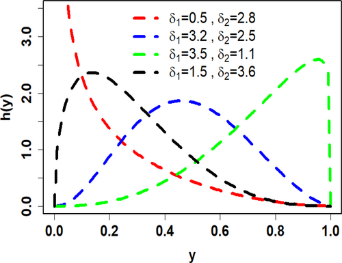
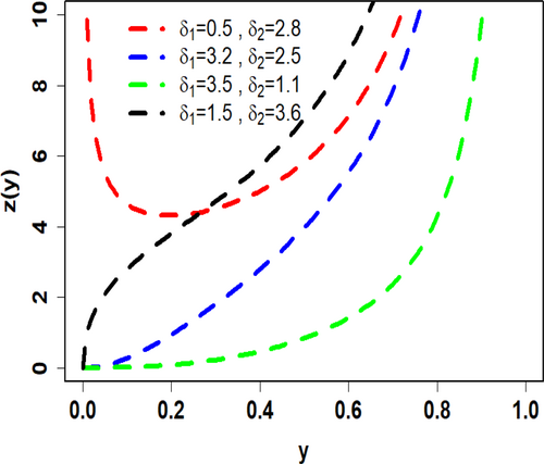
To visualize the shapes of the PDF (6) and HRF (7), Figures 1 and 2 depict their plots for varying values of the parameters and The PDF graphs, in Figure 1, for different combinations of parameters show a range of shapes, including reversed J-shaped, left-skewed, right-skewed, and unimodal. Significantly, depending on the parameter values, the HRF exhibits remarkable flexibility, showing growing, decreasing, bathtub, and j-shaped patterns (see Figure 2). This illustrates the great level of flexibility needed for various unit data analysis.
3 Characteristics of UIEP Distribution
Several important statistical properties of the UIEP distribution are examined in this section. Moments, IMs, QF, SO, PWM, and S-SR are some of these properties.
3.1 Probability Weighted Moments
3.2 Moments Measures
Numerical values for certain parameter values, (a) , (b) , (c) , (d) of the first four moments variance (), coefficient of Skewness (CS) and coefficient of Kurtosis (CK) of the UIEL distribution are listed in Table 1.
| Measures | Parameters | |||||||
|---|---|---|---|---|---|---|---|---|
| CS | CK | |||||||
| 0.5 | 0.5 | 0.4667 | 0.3397 | 0.2781 | 0.2403 | 0.1219 | 0.1353 | 1.5386 |
| 1.5 | 0.2608 | 0.1335 | 0.0847 | 0.0600 | 0.0655 | 0.9396 | 2.8384 | |
| 2 | 0.2146 | 0.0959 | 0.0548 | 0.0355 | 0.0498 | 1.1513 | 3.4939 | |
| 3 | 0.1587 | 0.0566 | 0.0269 | 0.0150 | 0.0314 | 1.4389 | 4.6253 | |
| 3 | 0.5 | 0.9000 | 0.8286 | 0.7738 | 0.7299 | 0.0186 | −2.1073 | 7.8661 |
| 1.5 | 0.6318 | 0.4417 | 0.3295 | 0.2573 | 0.0425 | −0.3642 | 2.3694 | |
| 2 | 0.5429 | 0.3357 | 0.2262 | 0.1619 | 0.0410 | −0.0711 | 2.2658 | |
| 3 | 0.4214 | 0.2110 | 0.1188 | 0.0728 | 0.0334 | 0.2798 | 2.4776 | |
Table 1 shows that the moment values increase, but the CS and values decrease when increases and keeps constant. Both platykurtic and leptokurtic distributions, as well as left- and right-skewed distributions, are possible for the UIEP. Figure 3 displays these patterns for 3D plots of , , CS, and CK.
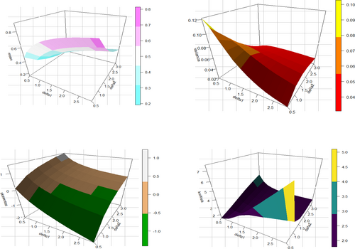
Figure 3 shows how the UIEP distribution is flexible in skewness and kurtosis. The skewness ranges from about −2 to 1, showing a wide variety of options. Furthermore, kurtosis can have both small and large values, allowing the distribution to display all three kurtosis types: leptokurtic, mesokurtic, and platykurtic. These results show how the PDF and HRF of the UIEP distribution may take on various forms.
3.3 Incomplete Moments
A distribution's IM offers important information beyond just means and variances. They highlight extreme occurrences by capturing the dynamics of tails and asymmetries. For thorough risk assessment and decision-making, this knowledge is essential. We can improve the efficacy of our statistical analysis and obtain a deeper knowledge of the underlying data by accepting IMs.
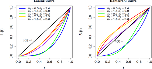
Figure 4 shows inequality differences between the Lorenz and Bonferroni curves for five groups that have different and values. The green curve, which represents the greatest inequality, is the farthest off the equality line in the Lorenz plot and has the lowest Bonferroni curve, particularly in the lower tail, showing that the lowest 20% of the population receives the smallest amount of income. Conversely, the gold curve displays the lowest inequality, with both curves closer to the equality line, showing a more balanced income distribution. Cods of Lorenz and Bonferroni curves are given in Appendix B.
3.4 Quantile Function
3.5 Stochastic Ordering
A foundational idea in probability theory, SO has been studied and used extensively for more than 40 years. Numerous domains, such as biological sciences, economics, insurance, survival analysis, queueing theory, and reliability engineering, find use for it. A useful tool for evaluating the robustness and performance of system components, this framework allows the comparison of non-negative continuous random variables.
It is obtained , at and , hence is a decreasing function and hence . Conclusions can also be made for various SO, like: hazard rate order , mean residual life order , SO , and reversed hazard rate order .
3.6 Stress-Strength Model
Note that the formula of S-SR of the UIEP given in Equation (13) is a function of the parameters .
4 Information Measures
5 Estimation Methods
In order to estimate parameters for the UIEP distribution, this section looks at five distinct approaches: ML, KO, AD, WLS, and LS. It also investigates the estimation of four entropy metrics for the UIEP distribution: AR, TS, Ré, and H–C. Each of these methods provides a unique method for estimating entropy measures and model parameters.
5.1 Maximum Likelihood Method
To estimate the unknown parameters and entropy measures of the UIEP distribution, the ML technique is used. Consider an observed simple random sample of size n, denoted by y1, y2,…, yn taken from the UIEP distribution. The log-likelihood function of the observed sample is given by
Notably, there are no closed-form solutions for Equations (23 and 24). Therefore, in order to derive the ML estimators of and of , numerical approaches using optim function in the R programming language are required. Furthermore, based on invariance property, the ML estimators of different entropy measures are produced after substituting and in Equations (16, 18, 20, and 22) to produce and .
5.2 Least Squares and Weighted Least Squares
Furthermore, the LS estimators of Ré, H–C, TS, and AR measures are produced, following the same procedure presented by Jha et al. [58], after substituting and in Equations (16, 18, 20, and 22) to produce and . Similarly, Furthermore, the WLS estimators of Ré, H–C, TS, and AR measures are produced after substituting and in Equations (16, 18, 20, and 22) to produce and .
5.3 Anderson–Dalring & Kolmogorov
The following non-linear equations are solved using an iterative method implemented in R, yielding the AD estimators and
Finally, the parameters and of the UIEP distribution are determined using the KO method. Maximizing the following equation, with respect to the parameters and to produce the KO estimators' parameters and is the aim of the following estimating procedure:
Also, the KO estimators and are produced after inserting and in Equations (16, 18, 20, and 22).
6 Numerical Simulation
- The true values on Table A1 are set1 = , while the corresponding true values of entropy measures are Ré = −0.40489, H–C = −0.55285, TS = −0.39680, and AR = −0.39592.
- The true values on Table A2 are set 2 = , white the associated true values of entropy measures are Ré = −0.61617, H–C = −0.83257, TS =0.59757, and AR = −0.59555.
- The true values on Table A3 are set 3 = , while the associated true values of entropy measures are Ré = −0.38956, H–C = −0.73420, TS = −0.43008, and AR = −0.41598.
- The true values Table A4. are set 4 = , while the associated true values of entropy measures are Ré =0.54937, H–C = −1.07929, TS =0.63223, and AR = −0.60289.
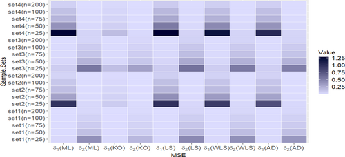
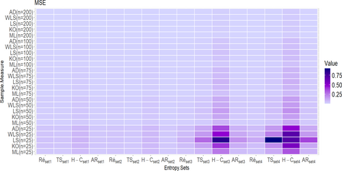
- As n increases, the ABs and MSEs of each estimate decrease.
- The KO method is the most efficient compared to all other estimation methods for the parameters of the UIEP distribution.
- As true values of and increase, the estimates for and generally show an increase in MSE across all methods.
- At , under the LS method, when is less than , the H–C entropy estimates show a higher increase in MSE than the TS entropy estimates. However, when is less than , the TS entropy estimate shows a higher increase in MSE than the H–C entropy estimate.
- At , the AR entropy estimation is the best compared to all other entropy estimation methods for the UIEP distribution.
- At , the Ré entropy estimation is the best compared to all other entropy estimation methods for the UIEP distribution.
- Both the AR and Ré entropy estimators are found to be best when using ML estimation. The AR estimate is preferred for low-entropy order value, whereas Ré is the superior choice for high-entropy order value.
7 Real Data Application
This section investigates the UIEP distribution by comparing it to well-known unit distributions available in the literature. For this comparison, two datasets are used: one with coronavirus data and one with rock samples from a petroleum reserve. The following distributions are examined for comparison: UEP distribution, UEL distribution, UEHL distribution, KW distribution, ETL distribution (Pourdarvish et al. [59]), ULL distribution, and UPL distribution.
- COVID Data
For an 82-day period in 2021, from May 1 to July 16, COVID-19 death rates were recorded in England (see Abu El Azm et al. [60]). The data are as follows: 0.0023, 0.0023, 0.0023, 0.0046, 0.0065, 0.0067, 0.0069, 0.0069, 0.0091, 0.0093, 0.0093, 0.0093, 0.0111, 0.0115, 0.0116, 0.0116, 0.0119, 0.0133, 0.0136, 0.0138, 0.0138, 0.0159, 0.0161, 0.0162, 0.0162, 0.0162, 0.0163, 0.0180, 0.0187, 0.0202, 0.0207, 0.0208, 0.0225, 0.0230, 0.0230, 0.0239, 0.0245, 0.0251, 0.0255, 0.0255, 0.0271, 0.0275, 0.0295, 0.0297, 0.0300, 0.0302, 0.0312, 0.0314, 0.0326, 0.0346, 0.0349, 0.0350, 0.0355, 0.0379, 0.0384, 0.0394, 0.0394, 0.0412, 0.0419, 0.0425, 0.0461, 0.0464, 0.0468, 0.0471, 0.0495, 0.0501, 0.0521, 0.0571, 0.0588, 0.0597, 0.0628, 0.0679, 0.0685, 0.0715, 0.0766, 0.0780, 0.0942, 0.0960, 0.0988, 0.1223, 0.1343, and 0.1781.
The COVID-19 data's key descriptive statistics are tabulated in Table 2 and visualized in Figure 7.
| Minimum | Maximum | SK | KU | |||||
|---|---|---|---|---|---|---|---|---|
| 0.002 | 0.014 | 0.027 | 0.036 | 0.046 | 0.178 | 0.001 | 2.021 | 8.176 |
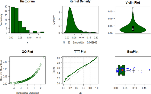
Figure 7 examines the total test time (TTT) plot and its relationship to HRF, demonstrating an excellent fit with the UIEP distribution. The PDF analysis shows asymmetrical data distribution. Quantile–quantile (QQ) and box plots are used to test normality and observe outliers, with the mean in red and outliers shown by blue rings on the plots. The left-hand panel of Table 3 shows the results of KO, LS, WLS, and AD estimation, along with their associated SEs, calculated specifically for the UIEP distribution. The right-hand panel of Table 3 presents the results of the ML estimation, including standard errors (SEs), for all distributions. Figure 8 illustrates a comparison of the SEs of different estimates for the UIEP distribution.
| Distribution | UIEP | UEP | UEL | UEHL | UG | ETL | ULL | UPL | ||||
|---|---|---|---|---|---|---|---|---|---|---|---|---|
| Methods | ML | KO | LS | WLS | AD | ML | ||||||
| 1.604 | 0.203 | 1.484 | 1.611 | 1.622 | 1.186 | 0.033 | 29.313 | 55.316 | 1.256 | 7.195 | 4.120 | |
| 36.161 | 1.139 | 35.381 | 37.499 | 37.613 | 0.087 | 41.763 | 1.251 | 1.238 | 24.979 | 3.597 | 1.868 | |
| — | — | — | — | — | 2.462 | 71.919 | — | — | — | — | 356.314 | |
| SE () | 0.257 | 0.026 | 1.222 | 0.054 | 0.481 | 0.096 | 0.016 | 9.285 | 18.084 | 0.111 | 0.662 | 0.383 |
| SE () | 4.725 | 0.111 | 23.935 | 1.023 | 8.819 | 0.343 | 18.526 | 0.103 | 0.105 | 6.944 | 0.096 | 0.665 |
| SE () | — | — | — | — | — | 11.530 | 26.624 | — | — | — | — | 115.113 |
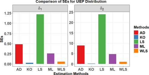
Table 4 and Figure 8 collectively indicate that the KO method offers the most reliable estimates, validating the simulation outcomes for the UIEP distribution. The goodness of fit measures as , , , , , , , and for the COVID-19 data are also shown in Table 4.
| Name | UIEP | UEP | UEL | UEHL | KW | ETL | ULL | UPL |
|---|---|---|---|---|---|---|---|---|
| −387.304 | −369.451 | −381.515 | −385.054 | −384.669 | −384.877 | −387.076 | −370.001 | |
| −382.491 | −362.231 | −374.295 | −380.241 | −379.856 | −380.063 | −382.063 | −362.781 | |
| −387.152 | −369.143 | −381.208 | −384.902 | −384.517 | −384.725 | −387.025 | −369.693 | |
| −385.372 | −366.552 | −378.617 | −383.122 | −382.737 | −382.944 | −385.144 | −367.102 | |
| 0.032 | 0.071 | 0.074 | 0.055 | 0.060 | 0.058 | 0.079 | 0.012 | |
| 0.244 | 0.494 | 0.509 | 0.393 | 0.421 | 0.411 | 0.749 | 0.109 | |
| 0.053 | 0.064 | 0.063 | 0.058 | 0.060 | 0.059 | 0.054 | 0.963 | |
| 0.974 | 0.886 | 0.901 | 0.949 | 0.931 | 0.938 | 0.969 | 0.054 |
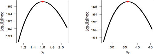
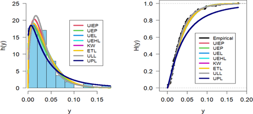
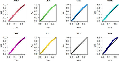
Figures 9-11 assess the UIEP distribution's fit to the COVID-19 data. Figure 9 shows the log-likelihood curve parameters for the UIEP distribution, which proves the estimators' maximizing. Figure 10 compares the estimated and empirical CDFs and the estimated PDFs with a histogram. Figure 11 displays a P–P plot of the UIEP distribution demonstrating the model's sufficiency.
- Petroleum Reservoir Data
There are 48 rock samples in the dataset, all taken from a petroleum reservoir discussed by Cordeiro and Brito [61]. The values for these samples are 0.0903296, 0.2036540, 0.2043140, 0.2808870, 0.1976530, 0.3286410, 0.1486220, 0.1623940, 0.2627270, 0.1794550, 0.3266350, 0.2300810, 0.1833120, 0.1509440, 0.2000710, 0.1918020, 0.1541920, 0.4641250, 0.1170630, 0.1481410, 0.1448100, 0.1330830, 0.2760160, 0.4204770, 0.1224170, 0.2285950, 0.1138520, 0.2252140, 0.1769690, 0.2007440, 0.1670450, 0.2316230, 0.2910290, 0.3412730, 0.4387120, 0.2626510, 0.1896510, 0.1725670, 0.2400770, 0.3116460, 0.1635860, 0.1824530, 0.1641270, 0.1534810, 0.1618650, 0.2760160, 0.2538320, and 0.2004470.
The petroleum reservoir data's key descriptive statistics are tabulated in Table 5 and visualized in Figure 12.
| Minimum | Maximum | SK | KU | |||||
|---|---|---|---|---|---|---|---|---|
| 0.090 | 0.162 | 0.199 | 0.218 | 0.263 | 0.464 | 0.007 | 1.169 | 4.110 |
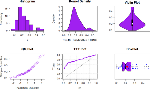
Following a summary of the petroleum reservoir data, Figure 12 examines the TTT plot and its relationship to HRF, demonstrating an excellent fit with the UIEP distribution. The PDF analysis shows asymmetrical data distribution. QQ and box plots are used to test normality and observe outliers, with the mean in red and outliers shown by blue rings on the plots. Table 6 displays the results of ML, KO, LS, WLS, and AD estimation, along with their associated SEs Figure 13 shows a comparison of the SEs of estimation methods for the UIEP distribution.
| Distribution | UIEP | UEP | UEL | UEHL | UG | ETL | ULL | UPL | ||||
|---|---|---|---|---|---|---|---|---|---|---|---|---|
| Methods | ML | KO | LS | WLS | AD | ML | ||||||
| 11.564 | 0.854 | 10.847 | 10.908 | 10.905 | 1.968 | 0.045 | 23.694 | 44.440 | 3.136 | 7.404 | 5.644 | |
| 12.285 | 2.291 | 12.373 | 12.267 | 12.235 | 0.298 | 63.783 | 2.746 | 2.715 | 13.641 | 1.582 | 4.164 | |
| — | — | — | — | — | 0.792 | 49.538 | — | — | — | — | 74.019 | |
| SE () | 3.891 | 0.065 | 21.015 | 1.058 | 7.149 | 0.199 | 0.035 | 8.954 | 17.444 | 0.364 | 0.898 | 0.870 |
| SE () | 1.625 | 0.115 | 8.936 | 0.461 | 2.990 | 2.942 | 45.985 | 0.285 | 0.293 | 4.199 | 0.053 | 3.389 |
| SE () | — | — | — | — | — | 15.365 | 20.603 | — | — | — | — | 52.583 |
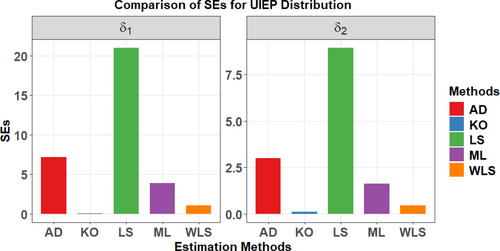
Analysis of Table 6 and Figure 13 demonstrates that the KO method provides the most accurate estimation, corroborating the simulation results for the UIEP distribution. The goodness of fit measures as , , , , , , , and for the petroleum reservoir data are also shown in Table 7.
| Name | UIEP | UEP | UEL | UEHL | UG | ETL | ULL | UPL |
|---|---|---|---|---|---|---|---|---|
| −110.825 | −45.004 | −98.266 | −101.451 | −100.983 | −102.712 | −106.497 | −110.169 | |
| −107.083 | −39.391 | −92.653 | −97.709 | −97.241 | −98.969 | −102.755 | −104.555 | |
| −110.559 | −44.459 | −97.721 | −101.184 | −100.716 | −102.445 | −106.230 | −109.623 | |
| −109.411 | −42.883 | −96.145 | −100.037 | −99.569 | −101.298 | −105.083 | −108.047 | |
| 0.072 | 0.281 | 0.218 | 0.201 | 0.208 | 0.187 | 0.127 | 0.096 | |
| 0.428 | 1.737 | 1.337 | 1.230 | 1.279 | 1.142 | 0.748 | 0.731 | |
| 0.117 | 0.159 | 0.154 | 0.150 | 0.153 | 0.153 | 0.212 | 0.389 | |
| 0.524 | 0.177 | 0.206 | 0.229 | 0.210 | 0.215 | 0.487 | 0.370 |
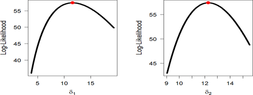
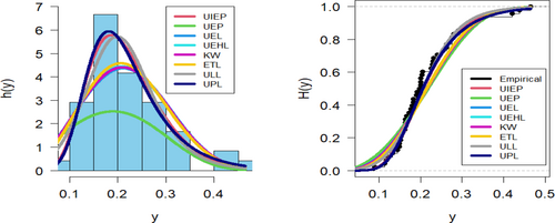
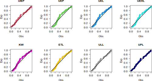
Figures 14-16 assess the UIEP distribution's fit to the COVID-19 data. Figure 14 shows the log-likelihood curve parameters for the UIEP distribution, which proves the estimators' maximizing. Figure 15 compares the estimated and empirical CDFs and the estimated PDFs with a histogram. Figure 16 displays a P–P plot of the UIEP distribution demonstrating the model's sufficiency.
8 Concluding Remarks
Unit distributions serve a key role in statistical modeling and are essential for assessing variables that are restricted to the interval [0,1]. In this study, we present the UIEP distribution, a new two-parameter model. Numerous forms are displayed by the UIEP, such as rising, J-shaped, or U-shaped hazard rate functions, as well as unimodal, reversed J-shaped, left-skewed, and right-skewed density functions. Its applicability for modeling unit data is improved by this flexibility. Quantiles, moments, PWM, SO, important uncertainty measures, Lorenz and Bonferroni curves, and the S-SR parameter are among the important statistical features that we derive analytically. To estimate distribution parameters and evaluate entropy measures, the statistical analysis uses a number of estimation approaches, such as ML, WLS, AD, LS, and KO. According to simulation data, the KO technique is the most successful estimation strategy among those studied for the parameters and entropy measures of the UIEP distribution. For lower entropy orders, the AR entropy typically performs better under ML estimation, whereas Ré entropy works better for higher entropy orders. This observation highlights a clear relationship between the entropy order and the optimal estimator. In order to verify the suggested distribution, we apply it to two real-world datasets: geological data from petroleum rock samples and health data associated with COVID-19. The model fit of these applications is better than that of other distributions. This study, although useful, has one drawback that should be noted. Primarily, this study utilizes four traditional estimation techniques along with large sample sizes. These methods are sensitive to small sample sizes, which can produce fewer stable estimates. The reliability of our conclusions may be impacted when working with smaller datasets, as this could result in less stable estimates or potentially prevent the model from converging. Future research could significantly benefit from exploring Bayesian estimation techniques. This approach is advantageous, especially when dealing with smaller samples, because it allows the use of informative priors and hierarchical modeling. Furthermore, implementing the UIEP distribution on real-world datasets with more complex structures would be essential in further verifying its practical usefulness.
Author Contributions
Amal S. Hassan: conceptualization, writing – original draft, writing – review and editing, methodology. Gaber Sallam Salem Abdalla: writing – original draft, writing – review and editing, conceptualization. Abdoulie Faal: writing – original draft, writing – review and editing, methodology. Omar A. Saudi: conceptualization, methodology, software, formal analysis, writing – original draft.
Acknowledgments
This work was supported and funded by the Deanship of Scientific Research at Imam Mohammad Ibn Saud Islamic University (IMSIU) (grant number IMSIU-DDRSP2501).
Conflicts of Interest
The authors declare no conflicts of interest.
Appendix A: See Table A1.
| n | True value | Ré (−0.40489) | TS (−0.39680) | H–C (−0.55285) | AR (−0.39592) | ||||||||
|---|---|---|---|---|---|---|---|---|---|---|---|---|---|
| Estimate | AB | MSE | AB | MSE | AB | MSE | AB | MSE | AB | MSE | AB | MSE | |
| 25 | MLE | 0.05340 | 0.02488 | 0.24693 | 0.40941 | 0.15783 | 0.04077 | 0.15059 | 0.03670 | 0.20981 | 0.07124 | 0.14981 | 0.03627 |
| KO | 0.02500 | 0.02209 | 0.06776 | 0.19170 | 0.17053 | 0.04943 | 0.16258 | 0.04430 | 0.22652 | 0.08600 | 0.16172 | 0.04377 | |
| LSE | 0.01297 | 0.02684 | 0.06432 | 0.44842 | 0.17465 | 0.05201 | 0.16618 | 0.04642 | 0.23153 | 0.09011 | 0.16526 | 0.04584 | |
| WLSE | 0.01993 | 0.02510 | 0.09651 | 0.41082 | 0.16781 | 0.04780 | 0.15980 | 0.04274 | 0.22264 | 0.08297 | 0.15893 | 0.04222 | |
| ADE | 0.02725 | 0.02250 | 0.13136 | 0.37353 | 0.16513 | 0.04574 | 0.15736 | 0.04099 | 0.21924 | 0.07958 | 0.15652 | 0.04050 | |
| 50 | MLE | 0.02336 | 0.00971 | 0.11835 | 0.15239 | 0.10927 | 0.01931 | 0.10456 | 0.01758 | 0.14567 | 0.03412 | 0.10405 | 0.01739 |
| KO | 0.00860 | 0.00936 | 0.03317 | 0.07818 | 0.12242 | 0.02458 | 0.11708 | 0.02231 | 0.16312 | 0.04332 | 0.11650 | 0.02208 | |
| LSE | 0.00551 | 0.01274 | 0.04028 | 0.19524 | 0.12285 | 0.02455 | 0.11739 | 0.02225 | 0.16355 | 0.04319 | 0.11680 | 0.02201 | |
| WLSE | 0.00983 | 0.01111 | 0.05896 | 0.16686 | 0.11667 | 0.02214 | 0.11154 | 0.02010 | 0.15541 | 0.03901 | 0.11099 | 0.01988 | |
| ADE | 0.01123 | 0.01005 | 0.06724 | 0.15494 | 0.11615 | 0.02180 | 0.11107 | 0.01980 | 0.15475 | 0.03844 | 0.11052 | 0.01959 | |
| 75 | MLE | 0.01429 | 0.00547 | 0.07256 | 0.08746 | 0.08907 | 0.01263 | 0.08533 | 0.01154 | 0.11889 | 0.02241 | 0.08493 | 0.01143 |
| KO | 0.00672 | 0.00559 | 0.03038 | 0.05539 | 0.09982 | 0.01604 | 0.09559 | 0.01463 | 0.13319 | 0.02841 | 0.09514 | 0.01449 | |
| LSE | 0.00168 | 0.00698 | 0.02289 | 0.11871 | 0.10011 | 0.01626 | 0.09580 | 0.01481 | 0.13347 | 0.02875 | 0.09533 | 0.01466 | |
| WLSE | 0.00554 | 0.00602 | 0.03888 | 0.10034 | 0.09509 | 0.01463 | 0.09103 | 0.01334 | 0.12683 | 0.02590 | 0.09059 | 0.01321 | |
| ADE | 0.00579 | 0.00567 | 0.03997 | 0.09212 | 0.09449 | 0.01439 | 0.09047 | 0.01313 | 0.12605 | 0.02549 | 0.09003 | 0.01300 | |
| 100 | MLE | 0.01272 | 0.00425 | 0.05338 | 0.05952 | 0.07624 | 0.00906 | 0.07312 | 0.00831 | 0.10188 | 0.01614 | 0.07278 | 0.00823 |
| KO | 0.00628 | 0.00415 | 0.02247 | 0.03687 | 0.08717 | 0.01182 | 0.08357 | 0.01082 | 0.11643 | 0.02101 | 0.08318 | 0.01072 | |
| LSE | 0.00249 | 0.00536 | 0.01372 | 0.08045 | 0.08703 | 0.01164 | 0.08339 | 0.01065 | 0.11618 | 0.02068 | 0.08299 | 0.01055 | |
| WLSE | 0.00588 | 0.00463 | 0.02734 | 0.06788 | 0.08217 | 0.01044 | 0.07877 | 0.00956 | 0.10974 | 0.01857 | 0.07840 | 0.00947 | |
| ADE | 0.00621 | 0.00448 | 0.02919 | 0.06465 | 0.08206 | 0.01039 | 0.07866 | 0.00953 | 0.10960 | 0.01849 | 0.07830 | 0.00943 | |
| 200 | MLE | 0.00549 | 0.00189 | 0.02550 | 0.02827 | 0.05363 | 0.00455 | 0.05146 | 0.00419 | 0.07170 | 0.00813 | 0.05122 | 0.00415 |
| KO | 0.00347 | 0.00201 | 0.01300 | 0.01871 | 0.06076 | 0.00584 | 0.05830 | 0.00537 | 0.08122 | 0.01042 | 0.05803 | 0.00532 | |
| LSE | 0.00114 | 0.00256 | 0.00718 | 0.04065 | 0.06030 | 0.00575 | 0.05784 | 0.00528 | 0.08058 | 0.01024 | 0.05757 | 0.00523 | |
| WLSE | 0.00295 | 0.00213 | 0.01492 | 0.03314 | 0.05737 | 0.00518 | 0.05504 | 0.00476 | 0.07669 | 0.00923 | 0.05479 | 0.00471 | |
| ADE | 0.00261 | 0.00209 | 0.01358 | 0.03190 | 0.05724 | 0.00516 | 0.05492 | 0.00474 | 0.07651 | 0.00920 | 0.05466 | 0.00469 | |
See Table A2
| n | True value | Ré (−0.61617) | TS (−0.59757) | H–C (−0.83257) | AR (−0.59555) | ||||||||
|---|---|---|---|---|---|---|---|---|---|---|---|---|---|
| Estimate | AB | MSE | AB | MSE | AB | MSE | AB | MSE | AB | MSE | AB | MSE | |
| 25 | ML | 0.36686 | 0.96741 | 0.05869 | 0.02876 | 0.16576 | 0.04412 | 0.15509 | 0.03828 | 0.21608 | 0.07431 | 0.15395 | 0.03768 |
| KO | 0.02098 | 0.08897 | 0.01186 | 0.01179 | 0.16889 | 0.04534 | 0.15825 | 0.03947 | 0.22049 | 0.07661 | 0.15712 | 0.03887 | |
| LS | 0.13045 | 0.98354 | 0.00439 | 0.02990 | 0.17638 | 0.04983 | 0.16494 | 0.04315 | 0.22981 | 0.08375 | 0.16372 | 0.04246 | |
| WLS | 0.16587 | 0.91525 | 0.01468 | 0.02728 | 0.17148 | 0.04742 | 0.16041 | 0.04110 | 0.22350 | 0.07979 | 0.15923 | 0.04046 | |
| AD | 0.20623 | 0.79717 | 0.02624 | 0.02610 | 0.16935 | 0.04582 | 0.15846 | 0.03976 | 0.22078 | 0.07718 | 0.15730 | 0.03914 | |
| 50 | ML | 0.16187 | 0.30968 | 0.02955 | 0.01183 | 0.11537 | 0.02137 | 0.10824 | 0.01872 | 0.15081 | 0.03634 | 0.10748 | 0.01845 |
| KO | 0.00556 | 0.05984 | 0.00748 | 0.00644 | 0.12120 | 0.02328 | 0.11378 | 0.02042 | 0.15853 | 0.03963 | 0.11299 | 0.02012 | |
| LS | 0.06454 | 0.41451 | 0.00531 | 0.01437 | 0.12417 | 0.02488 | 0.11644 | 0.02174 | 0.16224 | 0.04221 | 0.11562 | 0.02142 | |
| WLS | 0.08460 | 0.34898 | 0.01157 | 0.01253 | 0.11974 | 0.02320 | 0.11232 | 0.02029 | 0.15649 | 0.03940 | 0.11153 | 0.02000 | |
| AD | 0.09226 | 0.30718 | 0.01443 | 0.01182 | 0.11909 | 0.02271 | 0.11172 | 0.01989 | 0.15566 | 0.03860 | 0.11093 | 0.01960 | |
| 75 | ML | 0.09919 | 0.16256 | 0.01874 | 0.00707 | 0.09399 | 0.01397 | 0.08825 | 0.01227 | 0.12296 | 0.02383 | 0.08764 | 0.01210 |
| KO | 0.00910 | 0.03891 | 0.00657 | 0.00417 | 0.09735 | 0.01496 | 0.09147 | 0.01318 | 0.12744 | 0.02559 | 0.09084 | 0.01300 | |
| LS | 0.02996 | 0.21567 | 0.00279 | 0.00886 | 0.09984 | 0.01579 | 0.09375 | 0.01388 | 0.13062 | 0.02695 | 0.09310 | 0.01368 | |
| WLS | 0.04932 | 0.17876 | 0.00802 | 0.00765 | 0.09659 | 0.01481 | 0.09071 | 0.01303 | 0.12638 | 0.02529 | 0.09008 | 0.01284 | |
| AD | 0.05078 | 0.16306 | 0.00869 | 0.00721 | 0.09636 | 0.01471 | 0.09048 | 0.01293 | 0.12607 | 0.02511 | 0.08985 | 0.01275 | |
| 100 | ML | 0.08186 | 0.11689 | 0.01402 | 0.00489 | 0.08161 | 0.01055 | 0.07662 | 0.00927 | 0.10676 | 0.01799 | 0.07609 | 0.00914 |
| KO | 0.00421 | 0.02462 | 0.00322 | 0.00281 | 0.08661 | 0.01164 | 0.08137 | 0.01025 | 0.11337 | 0.01989 | 0.08081 | 0.01010 | |
| LS | 0.02614 | 0.15348 | 0.00144 | 0.00623 | 0.08829 | 0.01207 | 0.08291 | 0.01061 | 0.11552 | 0.02059 | 0.08233 | 0.01046 | |
| WLS | 0.04342 | 0.12828 | 0.00583 | 0.00533 | 0.08497 | 0.01129 | 0.07979 | 0.00992 | 0.11116 | 0.01926 | 0.07923 | 0.00978 | |
| AD | 0.04545 | 0.12290 | 0.00641 | 0.00516 | 0.08485 | 0.01123 | 0.07967 | 0.00987 | 0.11101 | 0.01917 | 0.07912 | 0.00973 | |
| 200 | ML | 0.03551 | 0.05016 | 0.00641 | 0.00237 | 0.05702 | 0.00515 | 0.05358 | 0.00454 | 0.07466 | 0.00882 | 0.05321 | 0.00448 |
| KO | 0.00884 | 0.01463 | 0.00298 | 0.00158 | 0.06014 | 0.00577 | 0.05652 | 0.00509 | 0.07875 | 0.00988 | 0.05613 | 0.00502 | |
| LS | 0.01239 | 0.07289 | 0.00072 | 0.00323 | 0.06180 | 0.00607 | 0.05807 | 0.00535 | 0.08090 | 0.01038 | 0.05767 | 0.00527 | |
| WLS | 0.02141 | 0.05840 | 0.00316 | 0.00269 | 0.05944 | 0.00560 | 0.05585 | 0.00494 | 0.07782 | 0.00958 | 0.05547 | 0.00487 | |
| AD | 0.01959 | 0.05626 | 0.00281 | 0.00260 | 0.05931 | 0.00558 | 0.05573 | 0.00492 | 0.07765 | 0.00955 | 0.05535 | 0.00485 | |
See Table A3
| n | True value | Ré (−0.38956) | TS (−0.43008) | H–C (−0.73420) | AR (−0.41598) | ||||||||
|---|---|---|---|---|---|---|---|---|---|---|---|---|---|
| Estimate | AB | MSE | AB | MSE | AB | MSE | AB | MSE | AB | MSE | AB | MSE | |
| 25 | ML | 0.10072 | 0.08191 | 0.27327 | 0.55313 | 0.15975 | 0.04703 | 0.20527 | 0.08657 | 0.35041 | 0.25227 | 0.18862 | 0.07026 |
| KO | 0.04484 | 0.15533 | 0.05854 | 0.31544 | 0.17961 | 0.06759 | 0.23620 | 0.14103 | 0.40321 | 0.41099 | 0.21518 | 0.10913 | |
| LS | 0.02762 | 0.08723 | 0.04758 | 0.58054 | 0.20319 | 0.09479 | 0.27762 | 0.29193 | 0.47393 | 0.85074 | 0.24898 | 0.18696 | |
| WLS | 0.03971 | 0.08129 | 0.08888 | 0.53128 | 0.18559 | 0.07289 | 0.24644 | 0.16474 | 0.42069 | 0.48009 | 0.22368 | 0.12284 | |
| AD | 0.05335 | 0.07217 | 0.13611 | 0.50253 | 0.17570 | 0.06190 | 0.22998 | 0.12790 | 0.39259 | 0.37274 | 0.20988 | 0.09899 | |
| 50 | ML | 0.04444 | 0.03029 | 0.13392 | 0.21739 | 0.10739 | 0.01961 | 0.13417 | 0.03205 | 0.22903 | 0.09341 | 0.12453 | 0.02717 |
| KO | 0.01335 | 0.02805 | 0.02924 | 0.11630 | 0.12149 | 0.02668 | 0.15312 | 0.04563 | 0.26139 | 0.13297 | 0.14167 | 0.03805 | |
| LS | 0.01277 | 0.04009 | 0.03541 | 0.26797 | 0.12805 | 0.03020 | 0.16262 | 0.05262 | 0.27760 | 0.15335 | 0.15007 | 0.04359 | |
| WLS | 0.02011 | 0.03457 | 0.06007 | 0.23212 | 0.11842 | 0.02488 | 0.14921 | 0.04199 | 0.25472 | 0.12236 | 0.13808 | 0.03519 | |
| AD | 0.02289 | 0.03100 | 0.07174 | 0.21825 | 0.11678 | 0.02378 | 0.14679 | 0.03978 | 0.25059 | 0.11592 | 0.13596 | 0.03344 | |
| 75 | ML | 0.02720 | 0.01667 | 0.08317 | 0.12749 | 0.08659 | 0.01260 | 0.10718 | 0.02002 | 0.18297 | 0.05834 | 0.09980 | 0.01714 |
| KO | 0.00857 | 0.01645 | 0.02433 | 0.08268 | 0.09669 | 0.01633 | 0.12038 | 0.02647 | 0.20550 | 0.07713 | 0.11186 | 0.02250 | |
| LS | 0.00480 | 0.02152 | 0.01964 | 0.16432 | 0.10160 | 0.01860 | 0.12725 | 0.03132 | 0.21722 | 0.09129 | 0.11800 | 0.02624 | |
| WLS | 0.01150 | 0.01832 | 0.04042 | 0.14088 | 0.09438 | 0.01554 | 0.11753 | 0.02533 | 0.20063 | 0.07383 | 0.10920 | 0.02148 | |
| AD | 0.01215 | 0.01710 | 0.04288 | 0.13144 | 0.09335 | 0.01506 | 0.11611 | 0.02439 | 0.19821 | 0.07107 | 0.10793 | 0.02073 | |
| 100 | ML | 0.02360 | 0.01268 | 0.06163 | 0.08754 | 0.07291 | 0.00857 | 0.08964 | 0.01326 | 0.15302 | 0.03864 | 0.08366 | 0.01146 |
| KO | 0.00749 | 0.01133 | 0.01555 | 0.05128 | 0.08339 | 0.01125 | 0.10288 | 0.01763 | 0.17562 | 0.05138 | 0.09590 | 0.01516 | |
| LS | 0.00547 | 0.01623 | 0.01125 | 0.11372 | 0.08569 | 0.01201 | 0.10611 | 0.01902 | 0.18114 | 0.05543 | 0.09879 | 0.01630 | |
| WLS | 0.01138 | 0.01386 | 0.02876 | 0.09699 | 0.07964 | 0.01023 | 0.09825 | 0.01599 | 0.16773 | 0.04661 | 0.09159 | 0.01377 | |
| AD | 0.01211 | 0.01337 | 0.03145 | 0.09329 | 0.07942 | 0.01014 | 0.09795 | 0.01583 | 0.16720 | 0.04613 | 0.09132 | 0.01363 | |
| 200 | ML | 0.01021 | 0.00558 | 0.02898 | 0.04206 | 0.05123 | 0.00424 | 0.06265 | 0.00643 | 0.10696 | 0.01873 | 0.05858 | 0.00559 |
| KO | 0.00458 | 0.00586 | 0.00988 | 0.02975 | 0.05709 | 0.00541 | 0.06996 | 0.00828 | 0.11943 | 0.02412 | 0.06537 | 0.00718 | |
| LS | 0.00254 | 0.00775 | 0.00586 | 0.05821 | 0.05805 | 0.00549 | 0.07122 | 0.00841 | 0.12157 | 0.02452 | 0.06652 | 0.00730 | |
| WLS | 0.00566 | 0.00636 | 0.01571 | 0.04817 | 0.05489 | 0.00484 | 0.06722 | 0.00737 | 0.11475 | 0.02147 | 0.06282 | 0.00640 | |
| AD | 0.00513 | 0.00620 | 0.01432 | 0.04653 | 0.05476 | 0.00483 | 0.06705 | 0.00734 | 0.11447 | 0.02140 | 0.06267 | 0.00638 | |
See Table A4
| n | True value | Ré (−0.54937) | TS (−0.63223) | H–C (−1.07929) | AR (−0.60289) | ||||||||
|---|---|---|---|---|---|---|---|---|---|---|---|---|---|
| Estimate | AB | MSE | AB | MSE | AB | MSE | AB | MSE | AB | MSE | AB | MSE | |
| 25 | ML | 0.42082 | 1.26243 | 0.07633 | 0.04901 | 0.17225 | 0.05401 | 0.23837 | 0.11824 | 0.40692 | 0.34456 | 0.21362 | 0.09022 |
| KO | 0.03616 | 0.16497 | 0.01603 | 0.02011 | 0.18521 | 0.06616 | 0.25917 | 0.19540 | 0.44244 | 0.56944 | 0.23095 | 0.12881 | |
| LS | 0.15341 | 1.27553 | 0.00520 | 0.05103 | 0.22446 | 0.12020 | 0.34359 | 0.93024 | 0.58654 | 0.71092 | 0.29423 | 0.37926 | |
| WLS | 0.19306 | 1.18734 | 0.01871 | 0.04652 | 0.20430 | 0.08595 | 0.29358 | 0.23877 | 0.50117 | 0.69584 | 0.25935 | 0.16526 | |
| AD | 0.23793 | 1.03226 | 0.03382 | 0.04448 | 0.19141 | 0.06930 | 0.26937 | 0.16560 | 0.45985 | 0.48258 | 0.23992 | 0.12209 | |
| 50 | ML | 0.18549 | 0.39709 | 0.03852 | 0.02021 | 0.11902 | 0.02370 | 0.15993 | 0.04506 | 0.27302 | 0.13131 | 0.14486 | 0.03628 |
| KO | 0.01904 | 0.07098 | 0.01196 | 0.00960 | 0.12845 | 0.02741 | 0.17248 | 0.05241 | 0.29445 | 0.15272 | 0.15625 | 0.04210 | |
| LS | 0.07606 | 0.53152 | 0.00670 | 0.02455 | 0.13600 | 0.03243 | 0.18517 | 0.06463 | 0.31610 | 0.18833 | 0.16695 | 0.05119 | |
| WLS | 0.09825 | 0.44642 | 0.01492 | 0.02140 | 0.12802 | 0.02817 | 0.17322 | 0.05488 | 0.29570 | 0.15993 | 0.15652 | 0.04381 | |
| AD | 0.10661 | 0.39221 | 0.01866 | 0.02019 | 0.12549 | 0.02685 | 0.16942 | 0.05186 | 0.28921 | 0.15113 | 0.15320 | 0.04153 | |
| 75 | ML | 0.11350 | 0.20727 | 0.02445 | 0.01208 | 0.09577 | 0.01520 | 0.12779 | 0.02793 | 0.21815 | 0.08140 | 0.11604 | 0.02277 |
| KO | 0.01381 | 0.04655 | 0.00882 | 0.00660 | 0.10290 | 0.01710 | 0.13695 | 0.03122 | 0.23379 | 0.09098 | 0.12446 | 0.02550 | |
| LS | 0.03578 | 0.27607 | 0.00349 | 0.01515 | 0.10624 | 0.01892 | 0.14257 | 0.03556 | 0.24339 | 0.10363 | 0.12921 | 0.02876 | |
| WLS | 0.05735 | 0.22807 | 0.01036 | 0.01308 | 0.10067 | 0.01690 | 0.13464 | 0.03130 | 0.22985 | 0.09121 | 0.12216 | 0.02545 | |
| AD | 0.05883 | 0.20742 | 0.01124 | 0.01232 | 0.10019 | 0.01668 | 0.13394 | 0.03086 | 0.22865 | 0.08993 | 0.12155 | 0.02510 | |
| 100 | ML | 0.09333 | 0.14814 | 0.01832 | 0.00836 | 0.08295 | 0.01104 | 0.11037 | 0.02007 | 0.18842 | 0.05848 | 0.10033 | 0.01642 |
| KO | 0.01722 | 0.03820 | 0.00699 | 0.00507 | 0.09149 | 0.01325 | 0.12162 | 0.02402 | 0.20761 | 0.06999 | 0.11058 | 0.01967 | |
| LS | 0.03068 | 0.19483 | 0.00178 | 0.01066 | 0.09188 | 0.01348 | 0.12265 | 0.02469 | 0.20937 | 0.07195 | 0.11136 | 0.02016 | |
| WLS | 0.04998 | 0.16255 | 0.00755 | 0.00912 | 0.08726 | 0.01221 | 0.11627 | 0.02224 | 0.19848 | 0.06481 | 0.10564 | 0.01819 | |
| AD | 0.05219 | 0.15563 | 0.00830 | 0.00883 | 0.08682 | 0.01208 | 0.11564 | 0.02198 | 0.19741 | 0.06407 | 0.10508 | 0.01798 | |
| 200 | ML | 0.04052 | 0.06336 | 0.00836 | 0.00406 | 0.05820 | 0.00545 | 0.07701 | 0.00967 | 0.13146 | 0.02817 | 0.07014 | 0.00798 |
| KO | 0.01201 | 0.02194 | 0.00399 | 0.00267 | 0.06348 | 0.00647 | 0.08399 | 0.01151 | 0.14338 | 0.03353 | 0.07650 | 0.00949 | |
| LS | 0.01457 | 0.09243 | 0.00088 | 0.00553 | 0.06417 | 0.00660 | 0.08510 | 0.01181 | 0.14527 | 0.03442 | 0.07745 | 0.00972 | |
| WLS | 0.02462 | 0.07390 | 0.00408 | 0.00461 | 0.06133 | 0.00600 | 0.08122 | 0.01067 | 0.13865 | 0.03109 | 0.07395 | 0.00880 | |
| AD | 0.02254 | 0.07112 | 0.00363 | 0.00445 | 0.06115 | 0.00597 | 0.08098 | 0.01063 | 0.13824 | 0.03098 | 0.07373 | 0.00877 | |
Appendix B:
See Appendix B
Coding in R of Lorenz and Bonferroni curves
library(ineq)
# Define parameter sets with distinct colors
params < - list
(list(delta1 = 0.5, delta2 = 2.4, color = “blue”),
list(delta1 = 1.4, delta2 = 0.8, color = “red”),
list(delta1 = 0.3, delta2 = 0.3, color = “green”),
list(delta1 = 2.5, delta2 = 2.5, color = “gold”),
list(delta1 = 1.5, delta2 = 2.3, color = “purple”)).
# Basic Probability Distribution Functions (PDF, CDF, Quantile)
fx < - function(x, delta1, delta2) {
delta1 * delta2 * (1 − x)^(delta2 − 1) * (1 − (1 − x)^delta2)^(delta1 − 1)
}
Fx < - function(x, delta1, delta2) {
(1 − (1 − x)^delta2)^delta1
}
Qx < - function(d, delta1, delta2) {
1 − (1 − d^(1/delta1))^(1/delta2)
}
# Functions for Inequality Curves
lorenz_curve < - function(samples) {
sorted_samples < - sort(samples)
cum_samples < - cumsum(sorted_samples)
total < - sum(sorted_samples)
L < - cum_samples/total
p < - seq(1/length(samples), 1, length.out = length(samples))
list(p = p, L = L)
}
bonferroni_curve < - function(lorenz_curve) {
B < - lorenz_curve$L/lorenz_curve$p
list(p = lorenz_curve$p, B = B)}
# Sample Generation
generate_samples < - function(param) {
n < - 10,000
u < - runif(n)
Qx(u, param$delta1, param$delta2)
}
# Plotting Setup
par(mfrow = c(1, 2), cex.main = 1.2, cex.lab = 1.5, cex.axis = 1.4,
mar = c(5, 5, 4, 2), mgp = c(3.5, 1, 0))
# Plotting Lorenz Curves
plot(NULL, type = “n”, xlim = c(0, 1), ylim = c(0, 1),
xlab = “t”, ylab = bquote({{L}}[F](t)), main = “Lorenz Curve”, lwd = 2)
for (param in params) {
samples < - generate_samples(param)
lc < - lorenz_curve(samples)
lines(lc$p, lc$L, col = param$color, lwd = 3.5)}
segments(0, 0, 1, 1, col = “black”, lty = 1, lwd = 3.5)
text(0.3, 0.32, expression(L(t) == t), pos = 2, cex = 1.2)
legend(“topleft”, legend = sapply(params, function(p) bquote(delta [1] == (p$delta1) ˜ delta [2] == (p$delta2))),
col = sapply(params, function(p) p$color), lwd = 4, bty = “n”, cex = 1.2)
# Plotting Bonferroni Curves
plot(NULL, type = “n”, xlim = c(0, 1), ylim = c(0, 1),
xlab = “t”, ylab = bquote({{B}}[F](t)), main = “Bonferroni Curve”, lwd = 2).
for (param in params) {
samples < - generate_samples(param).
lc < - lorenz_curve(samples).
bc < - bonferroni_curve(lc).
lines(bc$p, bc$B, col = param$color, lwd = 3.5)}
segments(0, 0, 1, 1, col = “black”, lty = 1, lwd = 3.5)
text(0.3, 0.3, expression(B(t) == t), pos = 4, cex = 1.2)
legend(“topleft”, legend = sapply(params, function(p) bquote(delta [1] == (p$delta1) ˜ delta [2] == (p$delta2))),
col = sapply(params, function(p) p$color), lwd = 4, bty = “n”, cex = 1.2)
########################## Goodness of Fit test ################################
#################clean up everything###############
remove(list = objects())
options(warn = −1)
#################Packages###############
library(stats4)
library(bbmle)
library(MASS)
library(AdequacyModel)
library(ggplot2)
######################## PDF and CDF of Distribution
##############define pdf and cdf for Unit inverse Exponentiated Pareto (UIEP) Distribution################
Pdf_UIEP < - function(parm,x){
delta1 < - parm[1]
delta2 < - parm[2]
Pdf_UIEP < - delta1 * delta2 * (1 − x)^(delta2 − 1) * (1 − (1 − x)^delta2)^(delta1 − 1)}
Cdf_UIEP < - function(parm,x){
delta1 < - parm[1]
delta2 < - parm[2]
Cdf_UIEP < - (1 − (1 − x)^delta2)^delta1}
#############define pdf and cdf for Unit Exponential Pareto (UEP) Distribution###############
Pdf_UEP < - function(parm,x){
delta1 < - parm[1]
delta2 < - parm[2]
delta3 < - parm[3]
Pdf_UEP < - (delta1 * delta3)/delta2*(x/(delta2 * (1 − x)))^(delta1 − 1)*exp(−delta3 * (x/(delta2 * (1 − x)))^delta1)}
Cdf_UEP < - function(parm,x){
delta1 < - parm[1]
delta2 < - parm[2]
delta3 < - parm[3]
Cdf_UEP < - 1 − exp(−delta3 * (x/(delta2 * (1 − x)))^delta1)}
########define pdf and cdf for unit exponentiated Lomax (UEL) Distribution
Pdf_UEL < - function(parm,x){
delta1 < - parm[1]
delta2 < - parm[2]
delta3 < - parm[3]
Pdf_UEL < - (delta1 * delta2 * delta3/x) * (1 − delta1 * log(x))^(−delta2 − 1) * (1 − (1 − delta1 * log(x))^(−delta2))^(delta3 − 1)}
Cdf_UEL < - function(parm,x){
delta1 < - parm[1]
delta2 < - parm[2]
delta3 < - parm[3]
Cdf_UEL < - (1-((1 − (1 − delta1 * log(x))^(−delta2))^(delta3)))}
#############define pdf and cdf for Unit-Exponentiated Half-Logistic (UEHL) Distribution ##########
Pdf_UEHL<- function(parm,x){
delta1 < - parm[1]
delta2 < - parm[2]
Pdf_UEHL<- (2 * delta1 * delta2 * x^(delta2 − 1))/((1 + x^delta2)^2) * ((1 − x^delta2)/(1 + x^delta2))^(delta1 − 1)}
Cdf_UEHL<- function(parm,x){
delta1 < - parm[1]
delta2 < - parm[2]
Cdf_UEHL < - 1 − ((1 − x^delta2)/(1 + x^delta2))^(delta1)}
############define pdf and cdf for umaraswamy Distribution (KW) Distribution ################.
Pdf_KW < - function(parm,x){
delta1 < - parm[1]
delta2 < - parm[2]
Pdf_KW < - (delta1*delta2)*(x^(delta1 − 1))*((1 − (x^delta1))^(delta2 − 1))}
Cdf_KW < - function(parm,x){
delta1 < - parm[1]
delta2 < - parm[2]
Cdf_KW < - 1 − ((1 − (x^delta1))^delta2)}
############## define pdf and cdf of Exponentiated Topp-Leone (ETL) Distribution
Pdf_ETL < - function(parm,x){
delta1 < - parm[1]
delta2 < - parm[2]
Pdf_ETL < -2 * delta1 * delta2 * (1 − x) * (x * (2 − x))^(delta1 − 1) * (1 − x^delta1 * (2 − x)^delta1)^(delta2 − 1)}
Cdf_ETL < - function(parm,x){
delta1 < - parm[1]
delta2 < - parm[2]
Cdf_ETL < - 1 − (1 − x^delta1 * (2 − x)^delta1)^(delta2)}
#############define pdf and cdf for unit log logistic (ULL) distribution ###############
Pdf_ULL < - function(parm,x){
delta1 < - parm[1]
delta2 < - parm[2]
Pdf_ULL < - (delta1/(x*delta2^delta1)) * (−log(x))^(delta1-1) * (1 + (−log(x)/delta2)^delta1)^(−2)}
Cdf_ULL < - function(parm,x){
delta1 < - parm[1]
delta2 < - parm[2]
Cdf_ULL < - (1 + (−log(x)/delta2)^delta1)^(−1)}
#############define pdf and cdf for unit power Lomax (UPL) Distribution###############
Pdf_UPL < - function(parm,x){
delta1 < - parm [1]
delta2 < - parm [2]
delta3 < - parm [3]
Pdf_UPL < - (delta1*delta2/(x*delta3))*((−log(x))^(delta1-1))*((1 + (1/delta3)*(−log(x))^delta1)^(−delta2 − 1))}
Cdf_UPL < - function(parm,x){
delta1 < - parm[1]
delta2 < - parm[2]
delta3 < - parm[3]
Cdf_UPL < - (1 + (1/delta3)*(−log(x))^delta1)^(−delta2)}
######################## Loglikelihood function ################################
LL_UIEP < - function(delta1,delta2){−sum(log(Pdf_UIEP(c(delta1,delta2),x)))}
LL_UEP < - function(delta1,delta2,delta3){−sum(log(Pdf_UEP(c(delta1,delta2,delta3),x)))}
LL_UEL < - function(delta1,delta2,delta3){−sum(log(Pdf_UEL(c(delta1,delta2,delta3),x)))}
LL_UEHL < - function(delta1,delta2){−sum(log(Pdf_UEHL(c(delta1,delta2),x)))}
LL_KW < - function(delta1,delta2){−sum(log(Pdf_KW(c(delta1,delta2),x)))}
LL_ETL < - function(delta1,delta2){−sum(log(Pdf_ETL(c(delta1,delta2),x)))}
LL_ULL < - function(delta1,delta2){−sum(log(Pdf_ULL(c(delta1,delta2),x)))}
LL_UPL < - function(delta1,delta2,delta3){−sum(log(Pdf_UPL(c(delta1,delta2,delta3),x)))}
############################# Real data #############################
################################################################################
x < - c(0.0903296, 0.2036540, 0.2043140, 0.2808870, 0.1976530, 0.3286410,
0.1486220, 0.1623940, 0.2627270, 0.1794550, 0.3266350, 0.2300810,
0.1833120, 0.1509440, 0.2000710, 0.1918020, 0.1541920, 0.4641250,
0.1170630, 0.1481410, 0.1448100, 0.1330830, 0.2760160, 0.4204770,
0.1224170, 0.2285950, 0.1138520, 0.2252140, 0.1769690, 0.2007440,
0.1670450, 0.2316230, 0.2910290, 0.3412730, 0.4387120, 0.2626510,
0.1896510, 0.1725670, 0.2400770, 0.3116460, 0.1635860, 0.1824530,
0.1641270, 0.1534810, 0.1618650, 0.2760160, 0.2538320, 0.2004470)
######## Maximum likelihood estimation for many distributions ##############
################################################################################
fit_UIEP < - mle2(minuslog = LL_UIEP,start = list(delta1 = 0.8,delta2 = 0.9),data = list(x), method = “BFGS”)
fit_UEP < - mle2(minuslog = LL_UEP,start = list(delta1 = 0.8,delta2 = 0.5,delta3 = 0.1),data = list(x), method = “BFGS”)
fit_UEL < - mle2(minuslog = LL_UEL,start = list(delta1 = 0.5,delta2 = 0.2,delta3 = 0.9),data = list(x), method = “BFGS”)
fit_UEHL < - mle2(minuslog = LL_UEHL,start = list(delta1 = 0.08,delta2 = 0.01),data = list(x), method = “BFGS”)
fit_KW < - mle2(minuslog = LL_KW,start = list(delta1 = 0.3,delta2 = 0.1),data = list(x), method = “BFGS”)
fit_ETL < - mle2(minuslog = LL_ETL,start = list(delta1 = 0.2,delta2 = 0.4),data = list(x), method = “BFGS”)
fit_ULL < - mle2(minuslog = LL_ULL,start = list(delta1 = 0.1,delta2 = 0.1),data = list(x), method = “BFGS”)
fit_UPL < - mle2(minuslog = LL_UPL,start = list(delta1 = 0.8,delta2 = 0.9,delta3 = 0.1),data = list(x), method = “BFGS”)
############Goodness of fit test##############
gof.test_UIEP < - goodness.fit(Pdf_UIEP,Cdf_UIEP,starts = c(coef(fit_UIEP)),data = x, method = “BFGS”, domain = c(0, 1))
gof.test_UEP < - goodness. fit(Pdf_UEP,Cdf_UEP,starts = c(coef(fit_UEP)),data = x, method = “BFGS”, domain = c(0, 1))
gof.test_UEL < - goodness. fit(Pdf_UEL,Cdf_UEL,starts = c(coef(fit_UEL)),data = x, method = “BFGS”, domain = c(0, 1))
gof.test_UEHL < - goodness.fit(Pdf_UEHL,Cdf_UEHL,starts = c(coef(fit_UEHL)),data = x, method = “BFGS”, domain = c(0, 1))
gof.test_KW < - goodness. fit(Pdf_KW,Cdf_KW,starts = c(coef(fit_KW)),data = x, method = “BFGS”, domain = c(0, 1))
gof.test_ETL < - goodness. fit(Pdf_ETL,Cdf_ETL,starts = c(coef(fit_ETL)),data = x, method = “BFGS”, domain = c(0,1))
gof.test_ULL < - goodness. fit(Pdf_ULL,Cdf_ULL,starts = c(coef(fit_ULL)),data = x, method = “BFGS”, domain = c(0, 1))
gof.test_UPL < - goodness. fit(Pdf_UPL,Cdf_UPL,starts = c(coef(fit_UPL)),data = x, method = “BFGS”, domain = c(0, 1))
################# Results######################
Name < - c(“UIEP”,”UEP”,”UEL”,”UEHL”,”KW”,”ETL”,”ULL”,”UPL”)
ParmI < - c(gof.test_UIEP$mle[1],gof.test_UEP$mle[1]
,gof.test_UEL$mle[1]
,gof.test_UEHL$mle[1]
,gof.test_KW$mle[1]
,gof.test_ETL$mle[1]
,gof.test_ULL$mle[1]
,gof.test_UPL$mle[1])
ParmII < - c(gof.test_UIEP$mle[2]
,gof.test_UEP$mle[2]
,gof.test_UEL$mle[2]
,gof.test_UEHL$mle[2]
,gof.test_KW$mle[2]
,gof.test_ETL$mle[2]
,gof.test_ULL$mle[2]
,gof.test_UPL$mle[2])
ParmIII < - c(gof.test_UIEP$mle[3]
,gof.test_UEP$mle[3]
,gof.test_UEL$mle[3]
,gof.test_UEHL$mle[3]
,gof.test_KW$mle[3]
,gof.test_ETL$mle[3]
,gof.test_ULL$mle[3]
,gof.test_UPL$mle[3])
St.Er_ParmI < - c(gof.test_UIEP$Erro[1]
,gof.test_UEP$Erro[1]
,gof.test_UEL$Erro[1]
,gof.test_UEHL$Erro[1]
,gof.test_KW$Erro[1]
,gof.test_ETL$Erro[1]
,gof.test_ULL$Erro[1]
,gof.test_UPL$Erro[1])
St.Er_ParmII < - c(gof.test_UIEP$Erro [2],gof.test_UEP$Erro[2]
,gof.test_UEL$Erro[2]
,gof.test_UEHL$Erro[2]
,gof.test_KW$Erro[2]
,gof.test_ETL$Erro[2]
,gof.test_ULL$Erro[2]
,gof.test_UPL$Erro[2])
St.Er_ParmIII < - c(gof.test_UIEP$Erro[3],gof.test_UEP$Erro[3]
,gof.test_UEL$Erro[3]
,gof.test_UEHL$Erro[3]
,gof.test_KW$Erro[3],gof.test_ETL$Erro[3]
,gof.test_ULL$Erro[3]
,gof.test_UPL$Erro[3])
ML < - c(gof.test_UIEP$Value,gof.test_UEP$Value
,gof.test_UEL$Value
,gof.test_UEHL$Value
,gof.test_KW$Value,gof.test_ETL$Value
,gof.test_ULL$Value
,gof.test_UPL$Value)
AIC < - c(gof.test_UIEP$AIC,gof.test_UEP$AIC
,gof.test_UEL$AIC
,gof.test_UEHL$AIC
,gof.test_KW$AIC,gof.test_ETL$AIC
,gof.test_ULL$AIC
,gof.test_UPL$AIC)
BIC < - c(gof.test_UIEP$BIC,gof.test_UEP$BIC
,gof.test_UEL$BIC
,gof.test_UEHL$BIC
,gof.test_KW$BIC,gof.test_ETL$BIC
,gof.test_ULL$BIC
,gof.test_UPL$BIC)
CAIC < - c(gof.test_UIEP$CAIC,gof.test_UEP$CAIC
,gof.test_UEL$CAIC
,gof.test_UEHL$CAIC
,gof.test_KW$CAIC,gof.test_ETL$CAIC
,gof.test_ULL$CAIC
,gof.test_UPL$CAIC)
HQIC < - c(gof.test_UIEP$HQIC,gof.test_UEP$HQIC
,gof.test_UEL$HQIC,gof.test_UEHL$HQIC
,gof.test_KW$HQIC,gof.test_ETL$HQIC
,gof.test_ULL$HQIC
,gof.test_UPL$HQIC)
KS < - c(gof.test_UIEP$KS$statistic,gof.test_UEP$KS$statistic
,gof.test_UEL$KS$statistic,gof.test_UEHL$KS$statistic
,gof.test_KW$KS$statistic,gof.test_ETL$KS$statistic
,gof.test_ULL$KS$statistic
,gof.test_UPL$KS$statistic)
P_value < - c(gof.test_UIEP$KS$p. value,gof.test_UEP$KS$p. value
,gof.test_UEL$KS$p. value,gof.test_UEHL$KS$p. value
,gof.test_KW$KS$p. value,gof.test_ETL$KS$p. value
,gof.test_ULL$KS$p. value
,gof.test_UPL$KS$p. value)
W < - c(gof.test_UIEP$W,gof.test_UEP$W
,gof.test_UEL$W
,gof.test_UEHL$W
,gof.test_KW$W
,gof.test_ETL$W
,gof.test_ULL$W
,gof.test_UPL$W)
A < - c(gof.test_UIEP$A,gof.test_UEP$A
,gof.test_UEL$A
,gof.test_UEHL$A
,gof.test_KW$A
,gof.test_ETL$A
,gof.test_ULL$A
,gof.test_UPL$A)
ResultsofMLE < - data.frame(Name,ParmI,ParmII,ParmIII,St.Er_ParmI,St.Er_ParmII,St.Er_ParmIII)
Resultsofgof < - data. frame(Name,ML,AIC,BIC,CAIC,HQIC,W,A,KS,P_value)
##########Graph of Histogram##########
data < - x
# Set larger font sizes globally
par(cex.axis = 1.2, cex.lab = 1.2, cex.main = 1.5, mfrow = c(1, 2), mar = c(5, 5, 4, 2),las = 1)
y < - seq(0, max(x), length. out = 1000)
hist(data, probability = TRUE,col = “skyblue”,ylim = c(0,7),xlim = c(min(x),max(x)), ylab = “h(y)”,xlab = “y”,main = “”)
lines(y, Pdf_UIEP(par < - gof.test_UIEP$mle,y), col = c(2),lwd = 3.5)
lines(y, Pdf_UEP(par < - gof.test_UEP$mle,y),col = c(3),lwd = 3.5)
lines(y, Pdf_UEL(par < - gof.test_UEL$mle,y), col = c(4),lwd = 3.5)
lines(y, Pdf_UEHL(par < - gof.test_UEHL$mle,y), col = c(5),lwd = 3.5)
lines(y, Pdf_KW(par < - gof.test_KW$mle,y), col = c(6),lwd = 3.5)
lines(y, Pdf_ETL(par < - gof.test_ETL$mle,y), col = c(7),lwd = 3.5)
lines(y, Pdf_ULL(par < - gof.test_ULL$mle,y), col = c(8),lwd = 3.5)
lines(y, Pdf_UPL(par < - gof.test_UPL$mle,y), col = “navy”,lwd = 3.5)
legend(0.28,7,horiz = F, c(“UIEP”,”UEP”,”UEL”,”UEHL”,”KW”,”ETL”,”ULL”,”UPL”), cex = 0.85,lty = 1,col = c(2,3,4,5,6,7,8,”navy”),lwd = 3.5)
#########Graph of Empirical cdf###########
plot(ecdf(data),verticals = TRUE, main = ““,ylab = “H(y)”,xlab = “y”)
lines(y,Cdf_UIEP(par < - gof.test_UIEP$mle,y), col = c(2),lwd = 3.5)
lines(y, Cdf_UEP(par < - gof.test_UEP$mle,y),col = c(3),lwd = 3.5)
lines(y, Cdf_UEL(par < - gof.test_UEL$mle,y), col = c(4),lwd = 3.5)
lines(y, Cdf_UEHL(par < - gof.test_UEHL$mle,y), col = c(5),lwd = 3.5)
lines(y, Cdf_KW(par < - gof.test_KW$mle,y), col = c(6),lwd = 3.5)
lines(y, Cdf_ETL(par < - gof.test_ETL$mle,y), col = c(7),lwd = 3.5)
lines(y, Cdf_ULL(par < - gof.test_ULL$mle,y), col = c(8),lwd = 3.5)
lines(y, Cdf_UPL(par < - gof.test_UPL$mle,y), col = “navy”,lwd = 3.5)
legend(0.25,0.58, c(“Empirical”,”UIEP”,”UEP”,”UEL”,”UEHL”,”KW”,”ETL”,”ULL”,”UPL”), cex = 0.85,lty = 1,col = c(1,2,3,4,5,6,7,8,”navy”),lwd = 3.5)
################# pp plot #################
par(cex.axis = 1.3, cex.lab = 1.3, cex.main = 1.3, mfrow = c(2, 4), mar = c(5, 5, 4, 2))
p < - (rank(x))/(length(x) + 1)
plot(Cdf_UIEP(par < - gof.test_UIEP$mle,x),p,type = “p”,pch = 1,xlim = c(0,1),ylim = c(0,1),col = 2,xlab = “Obs”,ylab = “Exp”, lwd = 4, main = “UIEP”)
par(new = TRUE)
segments(0,0,1,1, lwd = 2)
p < - (rank(x))/(length(x) + 1)
plot(Cdf_UEP(par < - gof.test_UEP$mle,x),p,type = “p”,pch = 1,xlim = c(0,1),ylim = c(0,1),col = 3,xlab = “Obs”,ylab = “Exp”, lwd = 4, main = “UEP”)
par(new = TRUE)
segments(0,0,1,1, lwd = 2)
p < - (rank(x))/(length(x) + 1)
plot(Cdf_UEL(par < − gof.test_UEL$mle,x),p,type = “p”,pch = 1,xlim = c(0,1),ylim = c(0,1),col = 4,xlab = “Obs”,ylab = “Exp”, lwd = 4, main = “UEL”)
par(new = TRUE)
segments(0,0,1,1, lwd = 2)
p < - (rank(x))/(length(x) + 1)
plot(Cdf_UEHL(par < - gof.test_UEHL$mle,x),p,type = “p”,pch = 1,xlim = c(0,1),ylim = c(0,1),col = 5,xlab = “Obs”,ylab = “Exp”, lwd = 4, main = “UEHL”)
par(new = TRUE)
segments(0,0,1,1, lwd = 2)
p < - (rank(x))/(length(x) + 1)
plot(Cdf_KW(par < - gof.test_KW$mle,x),p,type = “p”,pch = 1,xlim = c(0,1),ylim = c(0,1),col = 6,xlab = “Obs”,ylab = “Exp”, lwd = 4, main = “KW”)
par(new = TRUE)
segments(0,0,1,1, lwd = 2)
p < - (rank(x))/(length(x) + 1)
plot(Cdf_ETL(par < - gof.test_ETL$mle,x),p,type = “p”,pch = 1,xlim = c(0,1),ylim = c(0,1),col = 7,xlab = “Obs”,ylab = “Exp”, lwd = 4, main = “ETL”)
par(new = TRUE)
segments(0,0,1,1, lwd = 2)
p < - (rank(x))/(length(x) + 1)
plot(Cdf_ULL(par < - gof.test_ULL$mle,x),p,type = “p”,pch = 1,xlim = c(0,1),ylim = c(0,1),col = 8,xlab = “Obs”,ylab = “Exp”, lwd = 4, main = “ULL”)
par(new = TRUE)
segments(0,0,1,1, lwd = 2)
p < - (rank(x))/(length(x) + 1)
plot(Cdf_UPL(par < - gof.test_UPL$mle,x),p,type = “p”,pch = 1,xlim = c(0,1),ylim = c(0,1),col = “navy”,xlab = “Obs”,ylab = “Exp”, lwd = 4, main = “UPL”)
par(new = TRUE)
segments(0,0,1,1, lwd = 2)
ResultsofMLE
Resultsofgof
Open Research
Data Availability Statement
The data that support the findings of this study are available on request from the corresponding author. The data are not publicly available due to privacy or ethical restrictions.


