Hybrid CNN–LSTM Model With Soft Attention Mechanism for Short-Term Load Forecasting in Smart Grid
Funding: The authors received no specific funding for this work.
ABSTRACT
Integrating renewable energy in smart grids enables sustainable energy development but introduces challenges in supply–demand variability. Deep learning techniques are now imperative for Short-Term Load Forecasting (STLF), a significant enabler of energy flow management, demand-side flexibility, and grid stability. These methods optimize smart grid performance under variable conditions by leveraging the synergistic integration of multiple architectures. This paper proposes a novel hybrid CNN–LSTM parallel model with a soft attention mechanism to improve smart grids' STLF. The proposed model leverages Convolution Neural Networks (CNNs) to extract spatial patterns, LSTMs to capture temporal dependencies, and attention mechanisms to prioritize important information, enhancing predictive performance. A comprehensive comparative analysis uses two publicly available datasets, American Electric Power (AEP) and ISO New England (ISONE), to evaluate the proposed model's effectiveness. The proposed model provides outstanding performance across single-step and multistep forecasting operations by delivering the highest evaluation results. The proposed model delivered single-step forecasting results of 123.91 Root Mean Square Error (RMSE), 92.8 Mean Absolute Error (MAE), and 0.63 Mean Absolute Percentage Error (MAPE) on the AEP dataset and 126.16 RMSE, 64.28 MAE, and 0.44 MAPE on the ISONE dataset. The model delivered multistep forecasting results on AEP, which showed RMSE at 685.25, MAE of 490.37, and MAPE of 3.27, while ISONE produced RMSE of 598.26, MAE of 402.44, and MAPE of 2.73. The simulation results demonstrate that parallel CNN–LSTM with a soft attention mechanism effectively supports the development of adaptive and resilient smart grids, enabling better integration of renewable energy sources.
1 Introduction
Power utility industries must implement smart grid systems due to the changes needed to integrate Renewable Energy Sources (RESs) into the existing power systems. RESs have undergone a transition that led to new problems stemming from the unpredictable nature of their supply and demand because of their variable and intermittent characteristics [1]. STLF stands as a crucial power system operational need to deliver essential operational information for short-term grid management and resource flexibility, along with demand and supply balancing capabilities. Correct forecasting models protect smart grid decisions from failure, while accurate predictions help maximize RES use with stable grid operations [2, 3]. STLF implementations based on traditional techniques fail to account for time-related and spatial features that energy consumption follows. Deep learning models function in smart grid environments as complex structures for implementing practical applications. Hybrid deep learning models demonstrate high suitability for this field because they can recognize complicated patterns and adjust to multiple operational patterns of the smart grid [4]. This research proposes to improve STLF in smart grids by combining Convolutional Neural Networks (CNNs) and Long Short-Term Memory (LSTM) networks through a soft attention mechanism. The CNN network extracts spatial characteristics from energy information, and the LSTM network maintains temporal dependence information. Through its soft attention mechanism, the model gains the ability to recognize vital temporal patterns that enhance its forecasting performance. This system unites grid operational conditions with RES management solutions to achieve optimal results.
1.1 Literature Review
STLF has become a major research topic in energy management since its inception to improve power system stability and efficiency. Initially favored for STLF was Autoregressive Integrated Moving Average (ARIMA) together with Multiple Linear Regression (MLR) and Support Vector Machine (SVM) because of their simplicity and low computational complexity [5]. However, these methods sometimes fail to consider the load profile's nonlinear, stochastic characteristics, especially in systems with a high RES integration [6-8]. The uncertainties of RESs, including wind and solar power, aggravated the drawbacks of these methods and forced the reallocation of research toward techniques like machine learning and deep learning [9, 10]. The use of deep learning models in STLF increased steadily over time because of the capacity to identify sophisticated dependencies from a big dataset. Convolutional networks have been popular and recommended for extracting spatial features from time series data. For example, [11] showed that CNNs can extract local features in the energy use data, which are important for short-term forecasting. In the same way, LSTM networks, a Recurrent neural network (RNN), are very good at establishing dependencies and solving the vanishing gradient criticism of traditional RNNs [12]. Such work has exhibited that the LSTMs outcompete conventional models by offering the right estimations of the load demographics for successive short and long periods [13, 14].
To fully benefit from CNN and LSTM, researchers have suggested the integration of both architectures into one. For instance, [15] proposed a CNN–LSTM model for energy load forecasting that we see as providing a good capability of learning the spatial and temporal features of energy load data. Nonetheless, these hybrid models offer potential, but no measures prioritize the formerly identified characteristics in energy data, which hinders these models' performance in the conditions of smart grids [16, 17]. To overcome this limitation, new attention mechanisms have been included to let the model focus on pertinent regions of the input sequence. Proposed for the first time in the context of natural language processing, attention mechanisms have been incorporated to improve the energy forecasting models. For example, [18] used attention layers in RNNs for energy demand forecasting, enhancing the method's accuracy by receiving a self-adjustable vector that shows the relative emphasis to assign to the various time steps. However, a gap remains in the energy consumption data SC paradigm due to the lack of holistic models that integrate CNNs, LSTMs, and attention to efficiently harness the spatial, temporal, and feature-level relationships [19, 20]. Present studies also include insufficient studies that have validated different, large, real-life datasets, making generalizations of past models somewhat restricted. Further, the methods under investigation remain limited to systems with a considerable share of smart grids and RES, which results in a large gap in load prediction methods in such systems [21-24]. As a result of these drawbacks, this paper presents CNN–LSTM coupled with a soft attention mechanism to produce an effective method to capture spatiotemporal dependencies on energy data and facilitate dynamic feature selection with the intent of producing highly reliable and accurate STLF in relation to smart grids. Therefore, by executing the model on various real datasets, this study offers a complete approach to renewable energy integration challenges into new power systems.
1.2 Research Gap
The development of hybrid deep learning models for STLF remains in its developing stages, with several critical challenges yet to be addressed. Existing approaches often struggle to effectively capture and interpret the complex, interdependent spatiotemporal patterns inherent in energy datasets, particularly in scenarios involving high penetrations of distributed RESs. Despite their proven success in other domains, attention mechanisms remain underexplored in this context. Their integration with CNN–LSTM parallel architectures, in particular, has received limited investigation, presenting a significant opportunity to enhance forecasting accuracy through improved feature extraction and prioritized feature selection.
1.3 Paper Contributions
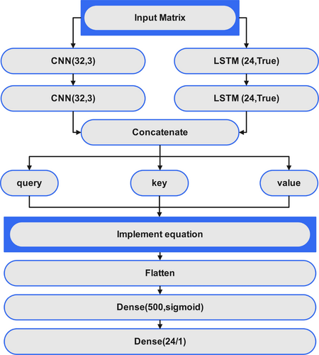
This study fills current research holes concerning STLF in smart grids through its presentation of a hybrid CNN–LSTM parallel model that operates with a soft attention mechanism. This model uses CNN–LSTM parallel structures to analyze spatial and temporal energy usage patterns in the consumed data. The forecasting performance of the model improves through the implementation of the soft attention mechanism, which selects vital temporal features. The proposed model underwent extensive comparison against other hybrid models to demonstrate its robust and general application possibilities. The proposed forecasting model constitutes the supreme choice between single and multistep applications because it achieves peak results with both AEP and ISONE datasets. The proposed model demonstrated superior outcomes in single-step forecasting by producing an RMSE score of 123.91 along with an MAE of 92.80 and MAPE of 0.63 on AEP data while delivering an RMSE mostly equal to 126.16, MAE of 64.28, and MAPE of 0.44 on ISONE data. The proposed model emerges as the best forecasting model from all methods that were evaluated through experimental testing. The proposed model showed strong performance across multiple time steps of forecasting by delivering an RMSE of 685.25 together with MAE of 490.37 and MAPE of 3.27 for AEP data and RMSE of 598.26, MAE of 402.44, and MAPE of 2.73 for ISONE. The proposed model achieves outstanding load prediction accuracy because it detects temporal relationships together with spatial patterns.
1.4 Paper Organization
The structure of this paper is as follows: Section 1.1 of this work contains a description of the CNN, LSTM, and the proposed CNN–LSTM parallel model with an attention layer. The preprocessing techniques are featured in Section 2. The comparative analysis is presented in Section 3; Section 4 contains the conclusion and implications of the study.
2 Forecasting Center in Smart Grid
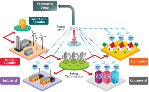
Figure 1 shows the forecasting mechanism of the smart grid. In the Forecasting Centre, RES data, which incorporates wind and solar and the usage of smart meters in commercial, residential, and industrial sectors, is employed. Predictive data also allows the smart grid operator to control energy distribution and not destabilize grids due to fluctuating RES. RES generators apply forecasting to optimize power management by maintaining a balance between conventional and renewable resources, and the power transmission system disburses electricity to various segments. This information is gathered from access points and smart meters and directly feeds the forecasting system, which allows for accurate demand and load management. This integration provides system control and grid performance, renewable power consumption, and energy control in the various sectors.
2.1 Proposed CNN–LSTM Model With Soft Attention Layer
2.2 CNN Architecture
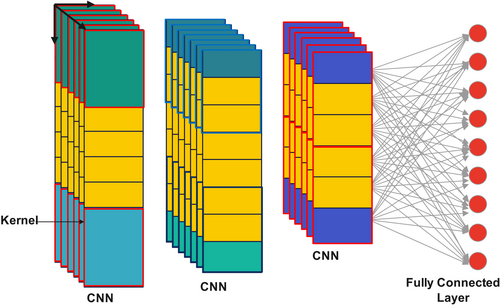
Figure 3 shows the structure of the CNNs. The CNN uses the filters (kernels) that move across the input to produce local features such as edges and texture and then assign those to new feature map locations containing areas of interest. The pooling layer mostly samples these feature maps in spatial dimensions using the max pooling layer. The main objective is to retain essential shapes while enhancing efficiency and making them invariant to spatial changes. The Fully Connected Layer flattens a feature map into a 1D vector, connecting every node to other neurons. Subsequently, the network blends the extracted features with complex findings. Finally, the output layer offers the best endpoint of the model for the problem being solved in question, whether that is classification or regression. CNNs are categories of ANNs that work specifically for text classification and picture and video recognition because of the advantages of handling high dimensionality. Some electrical systems in cars use smart sensors and goodies. Smart sensors and devices in the power system require storage of spatial information data; thus, a spatiotemporal matrix was constructed. Here, the nature of temporal and spatial correlation forms the basis for this matrix. Equation (2) presents the contingency spacetime revealed in Figure 3.
2.3 LSTM Models
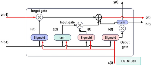
The LSTM cell in Figure 4 proposed for computational implementation is based on the long-term dependencies of sequential data and is specially designed for solving the vanishing gradient problem. It maintains two primary states: the cell state and the hidden state were both to be predicted. The LSTM uses three gates to regulate information flow: the forget gate, the input gate, and the output gate. Such gates utilize sigmoid and tanh activation to pass selective and adaptive data to the next layer. The and from above, the LSTM cell is updated and passed to the next LSTM cell to remember or forget information while addressing the vanishing gradient problem. The updated and are passed to the next LSTM cell, enabling it to remember or forget information dynamically. This form of architecture makes LSTMs particularly suitable for tasks such as time series analysis, natural language processing, and speech recognition because such models need to preserve necessary information while discarding unnecessary data.
3 Data Preprocessing
Data preprocessing effectively enhances the high quality of models and recognizes reliable patterns between data. The first stage involves data preprocessing, where the raw data is loaded, followed by data division. The data was split into three subsets: 60% for training, 20% for validation, and 20% for testing to ensure effective model development and evaluation. The correction activities usually performed when preparing the data for analysis include basic data cleaning, which covers cases such as the wrong format of dates, outliers, and missing values. Feature engineering concerns cyclic and noncyclic features, such as hours, days, months, holidays, seasons, and peak hours. The preprocessing includes MinMax normalization for numerical features; cyclical features are dealt with circularly(trigonometric transform), and categorical features are encoded using one-hot encoding. These features are then concatenated and reshaped into a format suitable for deep learning models: Samples, Time Steps, and Features. Two datasets were used in this research: AEP was used for the primary model training, while ISONE was used for validation.
Both datasets had missing data, categorized into three types: isolated missing values, several missing values consecutively, and a cluster of missing values. The missing data were addressed individually to maintain the original pattern and trend distributions. Table 1 shows the missing data in the AEP dataset, though the preprocessing steps of Figure 5 were carried out on both datasets. This consistent procedure made the model highly reliable and applicable to different tasks.
| Parameter | Value |
|---|---|
| Sample count before processing | 141,416 |
| Samples count with NaN | 0 |
| Duplicates | 4 |
| Missing values | 20 |
| Samples count after processing | 141,432 |

4 Result and Discussion
4.1 Dataset
The data sets used in this study are openly available [6]. Both datasets have hourly load data with their corresponding date and time. The model training was done on a PC using an Intel processor, RAM of 16 GB, and an NVIDIA GeForce RTX 2080 Graphics Card. Each training trial was consistently completed in approximately 16 min, highlighting the model's efficiency and suitability for processing large-scale energy datasets.
4.2 Results and Comparative Analysis
Training the models took two crucial steps to utilize the best performance of the model. The model was trained in the first phase involving 60 epochs, a batch size of 128, and a learning rate of using the Adam optimizer. A Keras callback was used to save the best model according to the minimum validation loss during this phase. In the second phase, the model selected from the experiment's first phase experienced further training with a learning rate of and batch size of 256 for 30 epochs. In the development process, Keras with backend Tensor Flow was used as the framework of choice, and Keras, in particular, has a well-established neural network component to ensure the stability of the model. It is worth saying that constant monitoring of the validation loss was critical to choosing the final model. This enhanced model was used in one-day load forecasting activities, capturing hourly and day-after electricity loading. Figure 6 illustrates various models' performance by showing their prediction accuracy against the actual load data while revealing their ability to match temporal load patterns. Each successive model depiction, starting with gray, cyan, blue, purple, and brown, shows substantial measurement errors, particularly during maximum and minimum load. Current models struggle to accurately predict key points when dealing with fast-temporal load variations because these variations lead to estimation results that wind up incorrect.
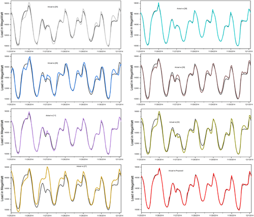
The proposed model (in red) provides outcomes with high precision that follow the actual loading pattern with minimal measurement deviations during all observation time. During quickly changing measurements, this model tracks both high and low points in the load cycle with high precision and accuracy. The proposed model shows advanced load dynamic forecasting capabilities because its design features excellent performance predictions. The robust model outcome establishes superior prediction accuracy over competing models, thus making it useful for operational short-term load prediction applications. The model achieves exact load pattern reflection because its advanced framework integrates temporal and spatial features into its attention-focused structure.
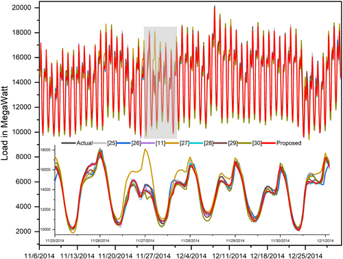
Figure 7 presents the accumulative comparisons of all the results. The figure displays an extensive comparison between actual and forecasted load data using various models while focusing on demonstrating the strong performance of the suggested red-colored model. The broader timeline view appears in the upper panel of the graph, followed by the lower panel, which displays daily sections for precise model performance examinations. The proposed model presents enhanced prediction accuracy compared to every model evaluated in the study (including [11, 25-30]) throughout all data measurement intervals. The proposed model shows a strong alignment between its red curve representation and the black actual load curve in the upper panel as it handles deviations observed in other models more effectively, especially during peak load and rapid fluctuations. Real-world forecasting benefits from the proposed model because it effectively reduces errors when loads are high. According to data captured in the lower panel analytical section, the proposed model demonstrates superior error reduction capabilities compared to alternative models. Unlike alternative methods, the proposed model tracks actual load trends while producing minimal deviation errors, frequently producing over- or underestimated load measurements. The accuracy of the proposed model remains consistently strong throughout the highlighted gray area as opposed to other models that display considerable deviations from actual measurements.
Furthermore, the study has compared the model performance with other state-of-the-art models using single-step and multistep forecasting. The analysis demonstrates that the proposed model delivers superior results when forecasting single-step and multi-step time series with AEP and ISONE datasets. The proposed model shows the lowest error metrics, surpassing all alternative models during single-step forecasting (Table 2).
| Model | AEP | ISONE | ||||
|---|---|---|---|---|---|---|
| Ref. no | RMSE | MAE | MAPE | RMSE | MAE | MAPE |
| [25] | 381.66 | 305.71 | 2.15 | 394.26 | 289.62 | 2.01 |
| [26] | 452.22 | 345.21 | 2.41 | 446.36 | 346.19 | 2.41 |
| [11] | 153.65 | 118.06 | 0.82 | 161.3 | 98.26 | 0.7 |
| [27] | 975 | 758.58 | 5.11 | 571.82 | 403.24 | 2.76 |
| [28] | 140.34 | 107.68 | 0.74 | 138.13 | 74.41 | 0.52 |
| [29] | 355.42 | 271.86 | 1.83 | 323.78 | 229.61 | 1.57 |
| [30] | 265.5 | 206.63 | 1.42 | 706.33 | 510.5 | 3.5 |
| Proposed | 123.91 | 92.8 | 0.63 | 126.16 | 64.28 | 0.44 |
The proposed model outperforms the next-best model [28] on the AEP dataset by achieving RMSE 123.91, MAE 92.8, and MAPE 0.63, while the other model produces values of 140.34, 107.68, and 0.74, respectively. The proposed model displays superior forecasting results on the ISONE dataset with an RMSE of 126.16, MAE of 64.28, and MAPE of 0.44 compared to [28], which reports an RMSE of 138.13 and MAE of 74.41 and MAPE of 0.52. The proposed model stands out by accurately identifying short-term dependencies in load forecasting, thus delivering the most accurate single-step predictions for all models evaluated.
In the same way, the proposed model demonstrates robust performance for multistep forecasting, as shown in Table 3, by maintaining superior outcomes compared to all competing approaches in predicting long-term dependencies. The proposed model yields an RMSE of 685.25 and MAE of 490.37 alongside a MAPE of 3.27 for the AEP dataset, which exceeds the next-best model ([11]) with an RMSE of 718.66 and MAE of 536.42 and MAPE of 3.64. The proposed forecasting framework generates scores of RMSE 598.26, MAE 402.44, and MAPE 2.73 while surpassing [28] because its RMSE and MAE results amount to 632.05 and 441.24, respectively, and its MAPE outcome stands at 3.01. The proposed model performs better when addressing complex forecasting situations by delivering precise predictions across extended periods. The proposed model consistently demonstrates superior performance on all forecast metrics for different datasets because it maintains both high precision accuracy and system robustness during real-world load forecasting operations. The model design demonstrates excellent scalability because it needs cost-effective training procedures for lightweight frameworks that enable large-scale deployments across numerous energy management solutions. The model displays generality functionality that supports various forecasting scenarios and different usage patterns based on multiple different dataset evaluations. Deployment challenges arise because real-time high-quality inputs are essential, along with integration capabilities for standard energy management systems. The maintenance of model quality under conceptual drift and usage pattern interruptions might sometimes need either retraining sessions or adaptational procedures.
| Model | AEP | ISONE | ||||
|---|---|---|---|---|---|---|
| Ref. no | RMSE | MAE | MAPE | RMSE | MAE | MAPE |
| [25] | 824.11 | 636.88 | 4.33 | 764.08 | 565.46 | 3.86 |
| [26] | 785.3 | 595.44 | 4.0 | 738.24 | 547.21 | 3.79 |
| [27] | 1262.83 | 982.4 | 6.66 | 851.78 | 638.78 | 4.36 |
| [11] | 718.66 | 536.42 | 3.64 | 659.7 | 466.13 | 3.2 |
| [28] | 772.3 | 574.57 | 3.87 | 632.05 | 441.24 | 3.01 |
| [29] | 790.1 | 580.23 | 3.86 | 726.47 | 499.96 | 3.39 |
| [30] | 735.31 | 553.3 | 3.73 | 706.33 | 510.5 | 3.5 |
| Proposed | 685.25 | 490.37 | 3.27 | 598.26 | 402.44 | 2.73 |
5 Conclusions
A novel deep learning model that combines CNN–LSTM alongside Soft Attention Mechanisms to develop accurate short-term load predictions in smart grid applications has been presented in this study. Through CNNs, the proposed model extracts spatial patterns simultaneously while LSTMs detect temporal correlations, and the attention mechanism focuses on essential information elements to reach improved prediction results. An evaluation across the AEP and ISONE datasets confirms that the proposed model delivers top performance in single-step and multistep forecasting while surpassing established models by producing minimum RMSE, MAE, and MAPE results. Single-step forecasting produced results with an AEP dataset RMSE of 123.91, MAE of 92.8, and MAPE of 0.63, along with an ISONE dataset RMSE of 126.16 and MAE of 64.28 and MAPE of 0.44, making it the most accurate forecasting model across all the comparisons. The proposed model demonstrates its ability to handle multistep forecasting scenarios by achieving an RMSE of 685.25, MAE of 490.37, and MAPE of 3.27 for the AEP dataset and an RMSE of 598.26, MAE of 402.44, and MAPE of 2.73 for the ISONE dataset. This methodology provides accurate load pattern predictions to develop adaptive smart grids that implement RESs better and enhance energy systems' stability and operational efficiency. Future research will study how to scale the model between multiple regions while combining forecasting data from various sources and weather and socioeconomic information to maximize accuracy.
Author Contributions
Syed Muhammad Hasanat: conceptualization, methodology, writing – original draft, software, data curation. Muhammad Haris: conceptualization, validation, writing – original draft, software. Kaleem Ullah: supervision, writing – original draft, visualization, investigation, formal analysis. Syed Zarak Shah: investigation, writing – review and editing, visualization, data curation. Usama Abid: formal analysis, writing – review and editing, validation, resources. Zahid Ullah: formal analysis, writing – review and editing, project administration, methodology, supervision.
Acknowledgments
The authors thank the Politecnico di Milano for open-access publishing under the CARE-CRUI Agreement. Open access publishing facilitated by Politecnico di Milano, as part of the Wiley - CRUI-CARE agreement.
Conflicts of Interest
The authors declare no conflicts of interest.
Open Research
Data Availability Statement
The data that support the findings of this study are available from the corresponding author upon reasonable request.


