Thermo-Electro-Mechanical Modeling of Failure: Application to Long-Term Reliability of Aging Transmission Lines
ABSTRACT
The integrity and reliability of a national power grid system are essential to society's development and security. Among the power grid components, transmission lines are critical due to exposure and vulnerability to severe external conditions, including high winds, ice, and extreme temperatures. The combined effects of external agents with high electrical load and the presence of damage precursors greatly affect the conducting material's properties due to a thermal runaway cycle that accelerates the aging process. In this paper, we develop a thermo-electro-mechanical model for long-term failure analysis of overhead transmission lines. A phase-field model of damage and fatigue, coupled with electrical and thermal modules, provides a detailed description of the conductor's temperature evolution. We define a limit state function based on maximum operating temperature to avoid excessive overheating and sagging. We study four representative scenarios deterministically and propose the Probabilistic Collocation Method (PCM) as a tool to understand the stochastic behavior of the system. We use PCM in forward parametric uncertainty quantification, global sensitivity analysis, and computation of failure probability curves in a straightforward and computationally efficient fashion, and we quantify the most influential parameters that affect failure predictability from a physics-based perspective.
1 Introduction
The power grid network in the United States is a complex and interconnected system. Despite its robustness, loss of single components can potentially lead to cascading failures [1-3] where the majority of disturbances are caused by natural events, such as storms, hurricanes, tornadoes, earthquakes, wildfire, and warming global temperatures [4, 5]. Given such complexity and apparent vulnerability, reliable prediction of system failure is of major importance. Identifying sensitive regions in the American power grid while predicting cascade failure is a challenging task, with significant national interest due to energy distribution and security concerns. A substantial number of stochastic inputs, such as weather, damage, and aging, dynamically influence such large-scale networks.
The reliability of transmission lines due to environmental effects has been studied in detail. Thermal failure in the form of overheating due to wildfires was studied in [6, 7]. In [8], the authors used a differential evolution algorithm to solve the inverse problem of parameter identification of heat equation parameters for overhead conductor temperature evolution. Damage in transmission lines and towers due to ice and wind loads was studied in [9] based on estimated generalized Pareto distributions of precipitation and wind loads. Other models studied the impact of severe weather on the reliability of transmission lines [10-12].
All those contributions are fundamental to a better understanding of transmission line reliability; however, they are limited in the specific scope of each work or are generally short-term simulations. The development of models that couple damage and fatigue mechanics formulations with the thermal and electrical aspects of the conductor could improve the predictability of transmission line failure for long-term operations.
In the field of fatigue and damage modeling, phase-field models are widely used, ranging from problems in brittle [13-16], ductile [17, 18], dynamic [19, 20], and non-isothermal fatigue fracture mechanisms [21]. The smooth crack representation in phase-field formulation naturally captures crack initiation, propagation, branching, and coalescence without explicit tracking of the crack geometry. More recently, damage phase-field models have incorporated electrical effects, yet they are restricted to piezoelectric applications [22, 23]. Other continuum damage approaches have been used in the context of electrical conductors [24], self-sensing materials [25], solder joints [26], and thermo-electro-mechanical wear of electrical contacts [27]. Yet, damage and fatigue effects on the thermo-electrical behavior of transmission line conductors and their impact on life-cycle prediction are still missing. Therefore, efficient and robust Uncertainty Quantification (UQ) and Sensitivity Analysis (SA) methods are essential.
Understanding the reliability of transmission lines requires an in-depth knowledge of the connections between mechanical, thermal, and electrical factors, as well as various sources of uncertainty. Although the phase-field model is commonly used to represent damage evolution, dislocation dynamics offers a detailed perspective on microstructural mechanisms [28]. Research indicates that interactions among dislocations significantly impact material properties and may contribute to failure under specific conditions [29, 30]. Additionally, at elevated temperatures, all materials diverge from Hooke's law, showing both viscous and elastic behavior. Recent developments in fractional visco-elasto-plastic models [31] provide a robust framework for capturing these behaviors in structural analysis [32], accurate modeling of damage progression [33], and large-scale system behavior [34]. Incorporating these fractional-order models improves predictions of transmission line failure by capturing more complex responses. For a comprehensive understanding of numerical techniques for fractional Ordinary and Partial Differential Equations, refer to [35]. Furthermore, fractional order can be considered an uncertain variable to model its associated randomness in system responses [36].
The complex system proposed in this paper cannot benefit from analytical integration during forward uncertainty quantification and sensitivity analysis (UQ/SA). This approach is typically effective only in simpler problems. Additionally, the system cannot rely on traditional sampling mechanisms in reliability engineering, such as the Monte Carlo method (MC) [37]. Different approaches have been proposed for the stochastic solution of Partial Differential Equations (PDEs) under parametric uncertainty. Methods such as Polynomial Chaos [38-40], or its generalization via Galerkin projections [41-43] suffer from being intrusive, as they directly modify the governing equations, thus have limitations in complex systems. The solution is to use non-intrusive methods, which use the forward deterministic solver as a black box. Traditional MC method [44, 45] computes moments of the Quantity of Interest (QoI) in a straightforward fashion yet is limited by slow convergence rates. Probabilistic Collocation Methods (PCM) [46, 47] promote an efficient computation of moments by direct numerical integration of QoI computed at the collocation points and yields faster convergence rates. Uncertainty quantification in the context of power grid systems has been discussed using PCM [48, 49] and Gaussian Processes [50], yet their focus is solely on the electrical short-term behavior. In damage phase-field applications, PCM has been effective in solving forward UQ and SA [51].
Recent studies have also highlighted the crucial role of dynamic thermal rating (DTR) systems in understanding transmission line aging. In particular, investigations on uncertainty in end-of-life failure and the impact of real-time thermal loading on reliability [52, 53] reveal how thermal effects and aging interact under dynamic conditions. Moreover, scenarios demonstrated in [54-58] underscore the versatility of DTR implementations from congestion management to renewable integration and cybersecurity. These studies provide valuable insights into the interplay between thermal loading and material aging. They offer promising directions for future research. However, our current work focuses on a coupled thermo-electro-mechanical model.
This work proposes a coupled thermo-electro-mechanical system with governing equations for displacements, material damage, material fatigue, temperature, and voltage. Initially, damaged conductor materials lead to overheating, affecting the mechanical load, subsequent aging, and increased resistivity, culminating in the premature failure of the transmission line. We use the PCM to transfer parametric uncertainty to the output of a physics-based model. We analyze how much each uncertain parameter affects the outcomes using sensitivity analysis and estimate the probability of failure over time across various scenarios, all through PCM.
- We propose a coupling between damage and fatigue based phase-field model with electrical and thermal effects that further drive the aging mechanisms.
- We employ the PCM beyond the uncertainty and sensitivity analyses, adopting the collocation method to compute directly the probability of failure when we transform the limit state function into a Bernoulli random variable that indicates failure.
- We study the system behavior and identify critical elements responsible for premature failure in different representative scenarios of damaged conductors, from normal operating conditions to seasonal high winds and increasing electric current and air temperature.
This work provides a robust connection between the detailed physical principles that govern mechanical, thermal, and electrical properties in a transmission line conductor and the probabilistic nature associated with uncertainties in parameters and loading conditions. For the first time, high-fidelity simulations of material aging are being used to provide predictive estimations of thermal failure probability.
This paper is organized as follows: in Section 2, we present the integrated model for the failure of transmission lines and discuss the temperature-based failure criterion. Then, we discuss the deterministic solution through the Finite-Element Method in Section 3, along with the definition of representative scenarios. The stochastic methods are discussed in Section 4, where we present the PCM building blocks for the uncertainty quantification, sensitivity analysis, and probability of failure. Finally, we address concluding remarks in Section 5.
2 Reliability of Transmission Lines
2.1 Problem Statement
Operating temperature is a critical indicator for the safe operation of transmission lines due to the risk of annealing the material components and excessive sagging during high-temperature conditions. Both outcomes pose serious consequences for the safety of surrounding areas and compromise the expected efficiency of electric energy transmission.
Complete cable rupture is a measure of transmission line failure that incurs inefficiency and repair costs. However, high operating temperatures–another indicator of failure–can be more dangerous because they might go unnoticed. Several conditions may contribute to an excess temperature operation, including an initial damaged state, aging of transmission line, increase in electric energy demand, and higher-than-normal air temperature conditions. Under these circumstances, the material temperature may exceed accepted values at specific points of the cable, significantly altering the prospect of a useful lifetime.
Therefore, the operating conductor temperature becomes the focal point of our analysis. The interplay between various physical effects, loading conditions, and material parameters will ultimately determine the transmission line's long-term failure. Our objective is to study the persistent multi-physics effect on the operating temperature of a transmission line with the presence of initial damage. To achieve such a long-term coupled system, several simplifying assumptions need to be made, which we will discuss in more detail in the next section.
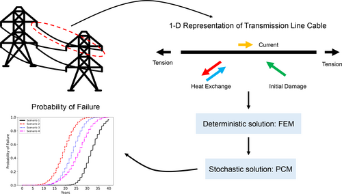
The thermo-electrical-mechanical model acts as the source of computation of , providing a high-fidelity measure of the maximum operating temperature across the cable through detailed simulations. Through the stochastic framework built on PCM, we obtain the probability of failure based simply on the physics at the material level. The overall flow of the proposed framework is illustrated in Figure 1.
2.2 Thermo-Electro-Mechanical Damage Phase-Field Model
We consider a transmission cable shown in Figure 1. Two transmission towers fix the cable, and sag is maintained below the maximum allowed threshold. From the mechanical perspective, we look at this system as a one-dimensional body under the influence of horizontal tension and consider the projected span as the operating length to keep the one-dimensional assumption. Sag is extremely important, and we take it into account when computing the tensile load due to temperature effects. However, we refrain from explicit sag modeling in this framework and focus solely on the tensile effects on the cable as drivers of material damage and fatigue.
The tension in the cable is driven primarily by its operating temperature. As it heats, the sag increases due to thermal elongation, which decreases the horizontal tension. Conversely, as the material cools, extra tension is induced by the contraction of the material.
Material temperature is a result of combined Joule heating from electric current and convective cooling from the ambient air with a given wind speed. In turn, higher temperatures are assumed to further degrade the material and enhance its aging process while affecting electrical conductivity and increasing resistivity.
With a focused look at the material behavior, the electrical component of the model is simplified and not related to the electrical design of transmission lines. Instead, the model is concerned with the effective electric current that passes through a single cable of the conductor and affects its material properties, regardless of the voltage level that the line provides to consumers. The ultimate effect of this consideration is that resistive losses along the line will heat the material and cause a voltage drop between its endpoints.
Finally, we assume that any damage to the material increases its resistivity. This additional degradation compounds the temperature effect on resistivity, leading to further energy dissipation through Joule heating. All the combined effects make the damage a precursor of a positive feedback loop of heating in the transmission line, causing early temperature failure due to compounding thermal runaway. In all physical components, we adopt a quasi-static perspective to allow for long-term simulations, such that in the proposed time scale, the system is assumed to reach equilibrium faster than changes in loading conditions.
2.2.1 Mechanical Model
Following the study by Boldrini et al. [21], our work models transmission line failure–including fatigue and damage–using a non-isothermal phase-field framework. This framework employs one Ordinary Differential Equation (ODE) to represent the fatigue variable and two Partial Differential Equations (PDEs) to evaluate the displacement field and damage field . The material degradation on the fractional scale is realized through , where refers to full fracture and refers to undamaged material. The degradation spectrum is quantified by the values of residing between 0 and 1, indicating partial damage. Damage evolves based on an Allen-Cahn type equation, derived along with the equilibrium equation for using virtual power principles and thermodynamic laws. The fatigue field is treated as an internal variable, with its evolution derived from constitutive relations that satisfy the entropy inequality.
We model the mechanical body in one dimension, occupying a domain at time . Specific material evolution forms arise from choosing appropriate free-energy potentials, one of which can be expressed as:
2.2.2 Thermal Model
represents the atmospheric pressure in , denotes the wind velocity in , and being the air and conductor's temperatures in , respectively, and is the conductor diameter in . We convert all parameters and the final (in ) to their respective SI units.
The specific form of will be discussed next.
2.2.3 Electrical Model
Transmission line design takes into account different effects such as AC frequency, inductance, reactance, and electromagnetic interactions with the air, ground, and nearby conductors, as well as electric load. In the end, those effects are crucial to determining the passing current across the conductor, yet they are out of the scope of the present study. Our study focuses on modeling the material's response to combined multi-physics effects rather than the design of the transmission line as an electric power component. Instead, we are interested in understanding how electricity-driven Joule heating affects a damaged material. In other words, we simply take the current as an input of the multi-physics system that could be obtained from other calculations.
Furthermore, the long-term analysis does not benefit from detailed time simulations of the transient effects of AC currents. The major focus is on the effect of damage-induced Joule heating. Therefore, the model refers to electric current as the DC-equivalent mean current that remains constant between consecutive time steps. This greatly simplifies the calculations, allowing for efficient measures of the quantities of interest, in this case, the heat source term. We adopt prescribed values for the current, yet they can be obtained from more sophisticated methods or from real-life data and used in this framework with no issues.
The presence of damage will disrupt the voltage field and will result in a different voltage drop between the extremities of the conductor.
In essence, the voltage drop will increase due to damage, incurring losses in electric power due to the decrease in conductivity of the conductor, further aggravating the thermal load to Joule heating.
2.3 Further Considerations for the Multi-Physics Model
As mentioned in the previous section, the horizontal tension in the cable is driven by temperature. When fixed at two points, cables sag in the shape of a catenary. There are diverse examples in the literature on simulation of their pure mechanical behavior [60, 61], yet here we adopt the simplifying assumption that our damage phase-field model is strictly 1-D. This means that we assume that the cable's length is sufficiently close to the span distance so that we can adopt them to be equivalent. This does not mean that sag is not present, but rather that the driver of mechanical damage and fatigue is solely the horizontal component of the cable tension, .
However, the effects of sag still need to be considered, especially under variable temperature conditions. Heat causes the length to increase, and the cable accommodates the elongation by increasing the sag, relieving some tension. On the other hand, the cable contracts in colder conditions, reducing sag and thus increasing tension. Therefore, mechanical load in the cable is a result of pre-tension in conjunction with tension changes due to the changes in the operating temperature. The mechanical loading is determined by the model itself.
2.4 Multi-Physics Framework
Figure 2 illustrates the current framework for computational failure modeling of the transmission line.
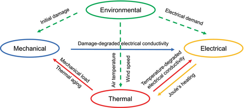
The system's governing equations are presented in Equations (4), (11), (6), (12), and (20). We also account for fatigue potentials, electrical conductivity degradation, and mechanical and thermal loading to accurately model the transmission line. Figure 2 shows how these mechanical, thermal, and electrical aspects are integrated. In addition, we include an abstract Environmental module in the computational domain to adjust the inputs and initial conditions to match real-world scenarios.
3 Deterministic Solution
This section outlines the Finite Element discretization of the current multi-physics model and presents the solution methodology within the deterministic framework. Such a deterministic framework serves both as a black box for non-intrusive stochastic methods in uncertainty quantification and analyzes the deterministic results, offering a clear basis for further assessments of uncertainty propagation across multiple dimensions.
3.1 Finite-Element Discretization
We adopt a staggered solution scheme to evaluate the equations in sequence at each time step. We summarize the procedure for deterministic solution in Algorithm 1
3.2 Representative Scenarios
- Scenario 1–Normal Operating Conditions: In this scenario, all loading conditions will follow an unchanged pattern throughout the years, and the only driver of material failure and, subsequently, of temperature increase is an initial damage precursor.
- Scenario 2–High Seasonal Winds: In this scenario, we simulate the aging and degradation of an initially damaged transmission line located in a region where one expects high winds during a specific season. For example, it could represent expected average winds over a few days during hurricane season or a known windy condition particular to a certain time of the year.
- Scenario 3–Increasing Electric Demand: Here, we simulate an increase in electric power demand in the region, which is driven by external factors that we do not address here. We model the effect of such factors in a linearly increasing average current over the years.
- Scenario 4–Increasing Air Temperature: The last scenario is concerned with the role of increasing ambient temperature over the course of several years, for example, as a result of climate change mechanisms, such that it decreases the rate of convective cooling and leads to early failure.
Note that all scenarios are long-term simulations of either slowly changing conditions or specific seasonal extreme events, such that there is no immediate effect in a time scale of minutes, hours, or even days. Yet they lead to accumulation of damage in the long run, making the conductor's life expectancy expire sooner than designed for normal operating conditions, whether with or without material damage.
3.3 Numerical Results
We defined the current cycle to correspond to higher demand in Winter and Summer and less demand during Spring and Fall. The definition of wind speed followed an arbitrary convention, possibly replacing it with a time-series data that best represents a region of interest. We represent tension in the horizontal direction by considering at and introducing the value of at . For damage, we adopt at the boundaries. For the current conservation equation, the boundary condition is similar to the mechanical case, and at , we are considering and applying a current density at .
Typical values for all parameters associated with a reference, normal condition (Scenario 1) simulation case are presented in Table 1.
| Parameter | Value | Unit |
|---|---|---|
| Length of cable | 200 | |
| # Elements | 1000 | |
| Diameter | 0.04 | |
| Initial damage intensity | 2.5 | — |
| Time-step for fatigue | 0.01 | |
| Young modulus | 69 | |
| Damage layer width | 0.02 | |
| Fracture energy | 10 | |
| Density | 2700 | |
| Aging coefficient | ||
| Thermal conductivity | 237 | |
| Electrical conductivity | ||
| Temperature coefficient | ||
| Pre-tension | 40 | |
| Base air temp | 288 | |
| Air temp amplitude | 10 | |
| Base wind speed | 2 | |
| Wind speed amplitude | 1 | |
| Base current | 1500 | |
| Current amplitude | 100 |
All simulations run up to 4000 time steps, representing a life cycle of 40 years. As the Aluminum conductor starts to anneal at temperature greater than 366 K [62, 63] and rapture if the temperature exceeds 373 K [64], so we consider the maximum limit temperature in the conductor at which all simulations are stopped to be = 373 K (100 C).
We start by investigating the evolution of field quantities in Scenario 1 under the reference parameters from Table 1. We plot field variables every 5 years in Figure 4.

We observe how damage initiates and concentrates in the region of a smaller cross-section area, thus driving an increase in temperature and a kink in the voltage fields. We also notice that due to damage and temperature increase, the voltage drop along the line increases with time as the conductor becomes more resistive.
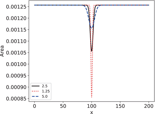
We can study the time evolution of maximum values by tracking the central node in the damage, fatigue, and temperature cases, as well as the maximum absolute voltage drop from the end node in the voltage field. Moreover, we compare the material behavior under different operating conditions, still under normal operations of Scenario 1. The most immediate comparison is to see the effect of initial damage represented by , Figure 5. It is evident that a sharper, intense variation in the area greatly reduces life, while a smoother variation does not make the material fail.

Next, we investigate the effects of wind, electric current, and air temperature in Figures 6-8, respectively.


An increase in the wind speed slightly advances the aging process, since more wind speed increases the load, accelerating the damage, at the same time it further cools the conductor, avoiding acceleration of temperature failure. The same competitive effects can be seen with the increase in temperature (in a warmer region), but the amplitude itself is not as influential since with more amplitude, there is also more cooling. However, the Joule heating from increasing the current base value and amplitude significantly reduces the expected life of the transmission line.
Even in Scenario 1, we see that normal operating conditions under different sets of external loads dramatically change the landscape of transmission line failure. Now, we investigate Scenarios 2, 3, and 4 with a closer focus on the maximum temperature time series, since it is the quantity of interest related to the failure criterion.
In Scenario 2, we simulate the presence of high seasonal wind through the parameter , applied between the 25th and 30th iterations of each year. The remainder of the year undergoes standard cyclic wind conditions, as in Scenario 1. Exclusively for Scenario 2, we choose . We compare the effects of initial damage at and different values of at reference parameters in Figure 9.
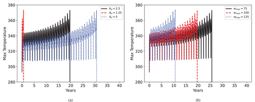
A more severe initial damage dramatically reduces the material's useful life. Furthermore, although high wind speeds enhance convective cooling, damage still accumulates over time. This accumulation eventually causes a concentration of damage at the center of the cable. As a result, the center overheats, which can lead to early failure. This is not a fast effect, like a cable snapping during a hurricane, but rather an acceleration of aging due to intense winds over several years.
Moving on to Scenario 3, we simulate a steady increase in the base electric current demand, parameterized by the rate of increase of current, , at each time-step, such that . This Scenario is representative of a region with an increasing population or growing industries, such that is chosen to provide a total increase of over 40 years when . Then, we observe the effect of initial damage at and different values of at reference parameters in Figure 10.
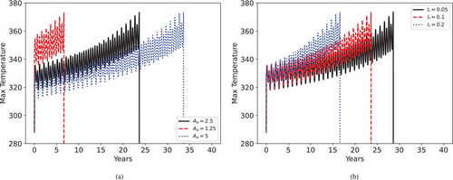
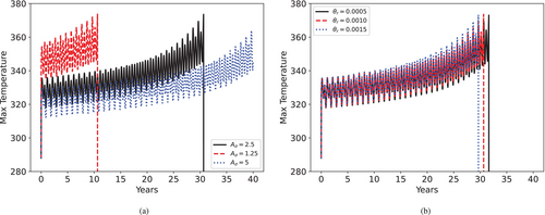
Last, we investigate the effects of the increase of base air temperature in Scenario 4, controlled by parameter . Similarly to Scenario 3, here we design to increment by . For a increase in 40 years, . In Figure 11, we see that even a slight increase in average yearly temperatures at reference parameters is sufficient to accelerate failure in transmission lines by a couple of years.
4 Stochastic Solution
We consider the deterministic model as a black box on which we can perform uncertainty quantification (UQ) and sensitivity analysis (SA). The use of non-intrusive methods is attractive since they allow us to use the same procedures from the deterministic solution for each realization of the stochastic problem. We use the Probabilistic Collocation Method to compute our quantity of interest (QoI).
Furthermore, the PCM is employed to perform the global sensitivity analysis through the computation of the Sobol Sensitivity Index in a computationally efficient way. The sensitivity index measures each parameter's importance in the QoI solution's total variance, and the PCM framework performs the computation through a simple post-processing task from UQ data.
Finally, the PCM building blocks are employed to facilitate the computation of directly from the first moment of a Bernoulli random variable defined directly from .
4.1 Uncertainty Quantification
We follow the methodology presented in [51] and assume be a complete probability space, where is the space of outcomes , is the -algebra and is a probability measure, . By treating the material and load parameters as random variables in a set , we make the transmission line model stochastic, such that the output temperature field also becomes a random variable. We represent the random parameters as .
A linear affine transformation from the standard domain to the real domain, , yields the Jacobian for one-dimensional integration as and gives the corresponding values of the random variable in the physical space.
We assume that the random variables are mutually independent and the discretization within the parametric space is isotropic. Additionally, we note that using a full tensor product, as applied in this project, is computationally efficient given the dimensionality is six or fewer. In high-dimensional stochastic spaces, Smolyak sparse grids [65] is a widely used approach to reduce the number of realizations needed while maintaining a similar level of accuracy. Other methods that aid uncertainty quantification (UQ) with dimensionality reduction include Principal Component Analysis (PCA) [66], low-rank approximations [67], and active subspace methods [68].
4.2 Sensitivity Analysis
The sensitivity indices measure the first-order effect on variance from , not taking into account interactions between and other parameters. From the normalization, , the remainder consisting of high-order interactions between the parameters, which we do not consider in this paper, but could be obtained in a similar fashion from post-processing of PCM [51].
The computation of could be quite challenging if the UQ is done through an MC method, yet here, the PCM acts as a building block for fast, cheap computations of global sensitivity.
4.3 Probability of Failure
In the final step, we aim to compute the probability of failure as a function of time. Existing methods to compute in reliability literature normally use MC to count the number of failure events [37]. Stochastic collocation methods provide only the moments of a limit state function . These moments must be transformed into a Probability Density Function (PDF). The PDF is then used to compute , similar to the approach in Equation (2). Such transformation from the moments to the PDF yields another level of complexity and can be done through methods of moments [71, 72], Polynomial Chaos [73, 74], Gaussian transformations [75] or optimization through entropy methods [76].
In this work, we propose an alternative to once again take advantage of the efficiency of PCM as a building block and obtain the probability of failure as a typical UQ expectation. Instead of computing moments of , obtaining an approximate PDF, and then computing , we first transform into another random variable , such that is Bernoulli with coefficient .
In practice, for each realization of PCM, we generate a time-series vector that is 0 until the point where , at which until the final time-step. For a single realization, this represents a step function at the failure point. When we consider the expectation of at a fixed time-step, then by the smoothness of the QoI becomes a real value .
Since we use PCM to compute the expectation of , which is a Bernoulli random variable, the expectation of gives , which is equivalent to the Bernoulli parameter itself. Therefore, a single integration using PCM is capable of providing an accurate measure of for each time step.
4.4 Numerical Results
With a deterministic simulation, we have a solid understanding of the effects of different parameters on the overall behavior of the system, including how shorter or longer the lifespan of the transmission line would be. We now focus on the effects of parametric uncertainty on maximum temperature. The parametric uncertainty is chosen to be a uniform distribution with a range of from the expected (mean) parameter value equal to the values used in the deterministic solution.
4.4.1 Preliminary Study: Scenario 1
We initially consider Scenario 1 as a point of reference to perform preliminary analyses on parametric and input load uncertainty. First, we perform UQ and SA on material parameters to identify the two most influential in the variance of . We focus on the set of material parameters that form the set that are either not accurately measurable or are an artifact of mathematical modeling. We assume all the other material parameters to be deterministic. In a separate stochastic space, we study the effect of loading conditions by looking into the set . We also select the top two most important from the global SA. Finally, we perform a final UQ/SA assessment with the 4 parameters selected in what we denote set . Later, those 4 parameters will be combined with specific scenario parameters in Scenarios 2, 3, and 4.
For all simulations, we consider PCM points per dimension. We also remark that in order to study the time-series results of maximum temperature among the entire stochastic space, we need to truncate the time-series minimum time of failure from all realizations since each realization observes failure at different times.
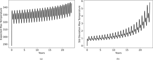
We start with the material parameter uncertainty from set and plot the evolution of the expected temperature field and its standard deviation over time in 5-year increments, and we plot the results in Figure 12.
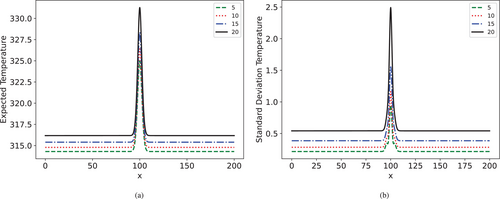
We can confirm that, indeed, the maximum temperature and maximum standard deviation will remain at the center as in the deterministic case. We then check the time-series evolution of the maximum temperature, obtained from the midpoint of the transmission line in Figure 13, and we note that the standard deviation grows with time.
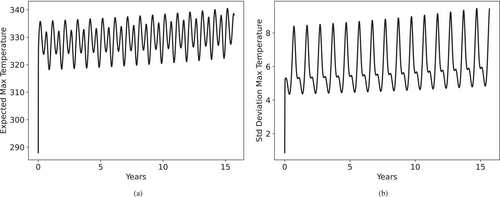
We plot the time-series evolution of maximum temperature for set in Figure 14, and we observe a more steady increase in the standard deviation, yet with higher amplitudes.
From the realizations obtained at the PCM collocation points, we compute the through Equation (86) and plot the time-series evolution of all parameters from both sets and in Figure 15.
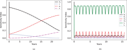
Within the material parametric set, that drives the damage localization is mostly important at the start of the simulation, where it initiates damage but then becomes unimportant. We see that and become important in the long run, as they are associated with the total energetic threshold for fracture and the rate of fatigue accumulation, respectively. Within the loading parametric set, the plays the most significant role in the overall uncertainty of because it directly influences Joule heating. The is the second most important due to the interplay between Joule heating and convective cooling.
We combine the most influential parameters from both and and form a new parametric space . Then, we perform a final round of SA for Scenario 1. We plot the results in Figure 16 and observe that loading conditions are more significant than material parameters from the beginning; however, the relative influence of material parameters grows with time as aging effects take place.

4.4.2 Convergence Analysis
Such results present an interesting perspective for the analysis of the remaining scenarios. Before we include the specific scenario parameters in the set of random variables, we check the consistency of preliminary PCM results by a convergence analysis. Due to the coupled, nonlinear nature of the deterministic problem, an analytical solution cannot be found, so we rely on a refined PCM solution as a reference.
We compute the all relative errors at year 25 and 10 years. The original time step was reduced by 10 times for a 25-year simulation run. The plots of the results are in Figure 17.

We see that PCM achieves a much lower error, around two orders of magnitude than 10000 MC realizations using only 5 points. This feature becomes even more important when we go to higher dimensions since MC would need a number of realizations with higher orders of magnitude to properly represent the high-dimensional parametric space. We have sufficient accuracy in PCM with 5 points, and we choose for all subsequent simulations in either 4-D or 5-D.
4.4.3 Scenarios 2, 3, and 4
In Scenarios 2, 3, and 4, we combine the 4 influential parameters from Scenario 1, set , with the corresponding parameter for each specific scenario, resulting in sets , , and , respectively.
In Scenario 2 the effect of the loading parameters is even more notable since the high winds drive damage faster and therefore do not leave time for aging to take place, as seen in Figure 18.

The scenario parameter of high wind speed with mean value has great importance when it initially hits the line, greatly increasing damage. Afterward, it does not have an impact as great as the first hit. Although the high wind speed lowers the temperature of the conductor significantly, the expected failure happens before 5 years.
Similarly, we observe that in Scenario 3, the mean value of also leads to more sensitivity in the loading conditions, especially the parameter, as seen in Figure 19.

Scenario 4, however, shows a surprising importance to the parameter that controls the rate of temperature increase, taken with mean value , Figure 20.

This result does not indicate whether the temperature increase itself leads to premature failure. Instead, it conveys the message that uncertainties in the prediction of significantly affect the uncertainties in predicting transmission line failure.
4.4.4 Probability of Failure
In this last part, we compute the expectation of Bernoulli variable as defined in Equation (87), and using the same PCM building block with , through the multi-dimensional expectation Equation (82). We plot the results for reference mean parameter values from sets , , , and in Figure 21.
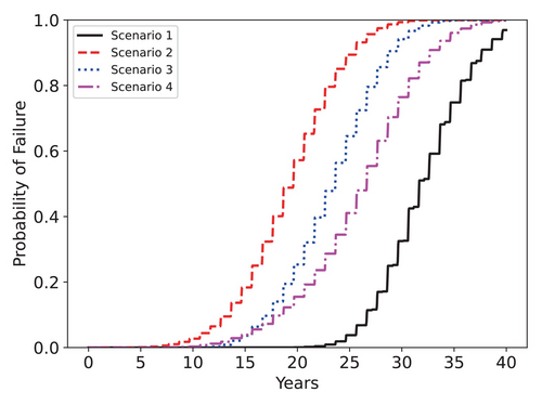
We see that normal operating conditions have the curve shifted to the right, while the more intense high wind scenario has the left-most failure curve. The average temperature increase has an interesting effect of increasing the probability of failure early on, followed by a rather smoother increase.
Finally, we compare the shape profiles of time-series on each Scenario by changing the mean value of specific parameters. In Scenario 1, we compare normal operation conditions for three levels of mean and their respective uncertainty bounds of . Similarly, we compare of Scenarios 2, 3, and 4 under different mean scenario parameters, namely , , and , respectively, and see how they shift. Unlike in previous SA of material parameters, such as and , or loads (which provide levels of importance with respect to their uncertainty), here we observe the effect of changing the base level of scenario parameters and initial damage and how they affect the curve. We plot the results in Figure 22

We observe distinct curve shapes in each scenario. For Scenario 1, the early failure of sharper initial damage is represented by a left shift of curve, while a smoother damage profile only leads to a chance of failure after 40 years. We observe similar effects for the parameters in Scenarios 2 and 3. For Scenario 4, a slight variation in the rate of base temperature increase is sufficient to increase the probability of failure of this particular line by to in 15 years. Although the increase in average temperatures may not be high individually, it is a global outcome compared to the region-specific failure prospects from Scenarios 2 and 3. Moreover, the combined effect of many transmission lines, each with a failure probability as low as , can compound and potentially lead to catastrophic power grid failure.
5 Conclusions
We developed a thermo-electro-mechanical model to analyze the failure in transmission lines. The mechanical model considers material damage evolution with long-term fatigue-driven aging mechanisms. The heat transfer equation includes Joule heating from electric current and convective cooling from the ambient environment. High temperatures accelerate aging and damage. This also affects the cable tension, which in turn compromises the material's conductivity. With this construction, an initially damaged transmission line conductor enters a positive feedback loop that leads to thermal runaway and failure when it reaches the material's annealing temperature.
- Quasi-static solutions of the thermo-electro-mechanical damage model are capable of simulating the long-term behavior of temperature cycles in the conductor, subject to time-changing conditions in wind, air temperature, and average electric current. We observe that slight changes in the initial damage or in the electric current may significantly reduce the life expectancy of the material.
- PCM is an accurate and cheap method that overcomes the main difficulties of MC methods. The tensorial product construction makes the computation of the global sensitivity index efficient. In the global SA, we observed the significant influence of electric current and rate of change of air temperature in the total variance of QoI.
- We further exploited the capabilities of PCM and computed the expectation of the Bernoulli random variable from PCM directly as a measure of the probability of failure.
We acknowledge that the current model relies on simplified assumptions. To provide a couple of examples, the assumption of quasi-static equations could be lifted in place of a transient analysis. Also, the simplification of the cable mechanics to one dimension could potentially be expanded to include the solution of the catenary shape as well. These and other assumptions could lead to a more complex system of equations better suited for each particular case, yet the overall framework and stochastic analysis structure would remain the same.
Nevertheless, we emphasize the potential of the proposed framework as a high-fidelity descriptor of probabilistic failure based on physical principles rather than pure mathematical modeling. The inclusion of real sensory data of wind speed, air temperature, and electric current for specific regions is straightforward and could lead to a more predictive estimation of failure probability. Through this construction, the reliability of transmission lines depends less on stochastic process modeling and instead benefits from detailed physics models of aging conductors.
Author Contributions
Eduardo A. Barros De Moraes: conceptualization; investigation; writing – original draft; methodology; validation; visualization; software; formal analysis; data curation. K. C. Prakash: writing – review and editing; validation; visualization; software; formal analysis; data curation; investigation. Mohsen Zayernouri: conceptualization; investigation; funding acquisition; writing – original draft; methodology; validation; visualization; formal analysis; project administration; supervision; resources.
Acknowledgments
This research was funded by the NSF award (DMS-1923201) and ARO Young Investigator Program (YIP) award (W911NF-19-1-0444).
Conflicts of Interest
The authors declare no conflicts of interest.
Open Research
Data Availability Statement
The data that support the findings of this study are available on request from the corresponding author. The data are not publicly available due to privacy or ethical restrictions.


