Prioritized Multi-Step Decision-Making Gray Wolf Optimization Algorithm for Engineering Applications
ABSTRACT
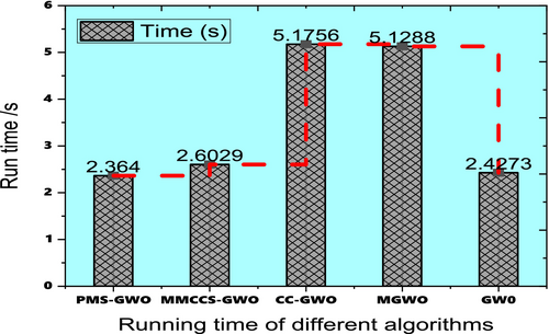
This article introduces the Prey-Movement Strategy Gray Wolf Optimizer (PMS-GWO), an enhanced version of the Gray Wolf Optimizer (GWO) designed to improve optimization efficiency through a novel multi-step decision-making process. By integrating adaptive exploration–exploitation strategies, PMS-GWO dynamically manages leadership roles, balances local and global searches, and introduces a prey escape mechanism, significantly improving solution diversity. Comparative analysis across 23 benchmark functions demonstrates PMS-GWO's superior performance, achieving up to 28.6% faster convergence and a 55.5%–93.8% increase in solution accuracy compared to the standard GWO. Notably, PMS-GWO enhances computational efficiency by 21.7%–27.4% and shows a 168.8% improvement in solution accuracy for the complex Michalewicz function over the baseline GWO. Visual convergence speed analysis, evidenced by a rapid fitness value decline within 100 iterations, reveals PMS-GWO's quickest convergence time of 0.02 s among tested algorithms. Furthermore, a comparison of runtime for several algorithms, including PMS-GWO, MMCCS-GWO, CC-GWO, MGWO, and GWO, clearly indicates that PMS-GWO achieves the lowest runtime of 2.364 s, significantly faster than CC-GWO and MGWO, which both exceed 5 s. This visual representation highlights the computational efficiency of PMS-GWO compared to other algorithms. PMS-GWO also outperforms advanced GWO variants like MMSCC-GWO, MGWO, and CCS-GWO, particularly in complex optimization landscapes, highlighting its adaptability and effectiveness for real-world applications in energy systems and engineering design. The multi-step decision-making process implemented in PMS-GWO is critical to achieving these improved convergence and diversity metrics.
1 Introduction
The rapid growth of renewable energy sources and the increasing complexity of modern energy systems necessitate advanced optimization techniques to enhance efficiency, reduce costs, and maintain system stability. Traditional optimization methods often fall short in addressing the dynamic and multi-objective nature of energy systems [1]. This has led to the development of metaheuristic algorithms, which offer more flexible and robust solutions. Among these, the Gray Wolf Optimization (GWO) algorithm has gained popularity due to its simplicity and effectiveness in solving various optimization problems [2]. Metaheuristics are methodical approaches designed to astutely explore the search space of optimization challenges to find close to optimal solutions [3]. These metaheuristic-based algorithms can be classified into two primary categories: neighborhood search-based and collective-based algorithms [4]. Additionally, they can be categorized into evolution-based algorithms, physics-based algorithms, chemistry-based algorithms, human-based algorithms, and swarm intelligence algorithms [5]. Local search algorithms begin with an initial solution and incrementally enhance it by investigating adjacent solutions [6]. Furthermore, GWO has been enhanced by integrating components from alternative optimization algorithms to enhance its effectiveness [7]. Moreover, hybridization with other optimization algorithms has been employed to strike a balance between exploration and exploitation capabilities, thereby enhancing the quality of GWO solutions [8]. Indeed, multiple variations of GWO are documented in the literature, each tailored to specialized search scenarios [9]. Wang et al. [10] introduced a novel modified iteration of the GWO algorithm to address the early convergence issue. Similarly, Hu et al. [11] proposed an altered version termed SCGWO, tailored for global optimization and feature selection (FS) challenges. Another chaotic adaptation of GWO was suggested by Zhang and Hong [12] for electric charge estimation. In Reference [13], Meidani et al. presented an inventive method to enhance the Gray Wolf Optimizer (GWO) through adaptive mechanisms. Saxena et al. [14] introduced a novel approach with a chaotic variant of the GWO algorithm for unconstrained numerical optimization. Likewise, Dhar et al. [15] presented an innovative and refined edition of the GWO algorithm known as CMA-GWO. A dynamically adjusted GWO was proposed by Yan et al. [16]. Wang et al. [10] proposed a fresh modified version of the GWO algorithm to address the early convergence challenge. Metaheuristics are high-level search strategies designed to approximate optimal solutions to complex problems. They can be categorized into two primary types: local search and population-based approaches. Local search methods iteratively improve a single solution by exploring its neighboring solutions, while population-based methods maintain a group of solutions and evolve them over time. Examples of local search techniques include simulated annealing, tabu search, and hill-climbing [17]. Metaheuristics can be categorized into several groups based on their underlying inspiration. Evolutionary algorithms simulate natural selection processes, employing techniques like mutation, crossover, and selection. Physics and chemistry-inspired algorithms leverage principles from these domains, such as gravity, thermodynamics, and chemical reactions. Social and human-based algorithms draw parallels with human behavior or societal structures. Finally, swarm intelligence algorithms mimic the collective behavior of animal groups, focusing on interactions within the population [18]. Swarm intelligence (SI) algorithms model collective behaviors observed in nature to solve optimization problems. These algorithms typically involve a population of agents that interact and collaborate to find optimal solutions [19]. Prominent examples include Particle Swarm Optimization, Ant Colony Optimization, and the Gray Wolf Optimizer (GWO). GWO, inspired by gray wolf hunting behavior, has gained significant attention due to its effectiveness in balancing the exploration and exploitation phases of the search process [20]. This adaptability has made GWO a versatile tool across various application domains. The Gray Wolf Optimizer (GWO) has undergone significant refinements to address the complexities of real-world optimization problems. Hybrid approaches and algorithmic enhancements have improved GWO's performance in constrained and non-convex scenarios. While GWO effectively balances exploration and exploitation through its hierarchical structure, its optimization efficiency can be further improved [21]. Inspired by the intricate communication dynamics within wolf packs, we propose a novel Prioritized Multi-Step Gray Wolf Optimization (PMS-GWO) that incorporates a more sophisticated interaction model between pack members. This refinement aims to enhance GWO's ability to converge to high-quality solutions [22]. The Gray Wolf Optimizer (GWO) is a swarm intelligence algorithm inspired by the hunting strategies of gray wolves. Introduced by Mirjalili et al. [23], GWO has gained significant popularity due to its simplicity, efficiency, and adaptability. By mimicking the hierarchical structure of a wolf pack, GWO effectively balances the exploration and exploitation phases during the search process. This enables it to tackle a diverse array of optimization challenges across various domains, including image processing, networking, and engineering [24]. To address the complexities of real-world optimization problems, the Gray Wolf Optimizer (GWO) has undergone significant refinement. By incorporating elements from other optimization techniques and tailoring its structure to specific problem domains, GWO has evolved into a powerful and versatile tool. These advancements have enabled the algorithm to effectively handle constrained, non-convex, and multi-objective optimization challenges. A multitude of GWO variants have emerged to tackle diverse research applications. The Gray Wolf Optimizer (GWO) initializes by randomly generating a population of wolves, which are hierarchically structured into alpha, beta, delta, and omega wolves [25]. Alpha wolves represent the best solutions, while beta and delta wolves occupy subsequent leadership positions. The remaining wolves, or omegas, follow the top three. GWO simulates the pack's hunting behavior by iteratively updating the positions of omega wolves based on their proximity to the leaders. This process involves a combination of encircling, tracking, and hunting strategies, carefully balanced by control parameters to optimize exploration and exploitation. GWO has emerged as a popular metaheuristic algorithm due to its effectiveness in addressing various optimization challenges [26]. However, its performance can be hindered by premature convergence. Inspired by the intricate communication dynamics observed in real wolf packs, we propose a novel optimization algorithm termed Prioritized Multi-Step Gray Wolf Optimization (PMS-GWO). This approach incorporates a detailed simulation of wolf pack behavior, including frequent information exchange between leaders and pack members during the hunt, aiming to enhance GWO's exploration and exploitation capabilities.
Despite its advantages, the standard GWO algorithm can be limited in handling complex, multi-objective optimization tasks required for modern energy systems. To address these limitations, we propose the Prioritized Multi-Step Decision-Making Gray Wolf Optimization (PMS-GWO) algorithm. The PMS-GWO enhances the traditional GWO by integrating a multi-step decision-making process that prioritizes key objectives such as cost minimization, load balancing, and the maximization of renewable energy utilization.
The PMS-GWO algorithm operates through a hierarchical decision-making framework that dynamically adapts to changing conditions and prioritizes decisions based on real-time data. This approach allows for more efficient and effective optimization of energy systems, ensuring better performance in terms of operational costs, load management, and renewable energy integration.
As demonstrated in the accompanying bar graph Figure 29, PMS-GWO achieves a significantly lower runtime of 2.364 s compared to other algorithms like CC-GWO and MGWO, which exceed 5 s, highlighting its computational efficiency. This runtime advantage is not only numerically significant but also crucial for real-time applications where computational speed is paramount. The simulation visually emphasizes this point by showing a clear separation between the runtime of PMS-GWO and the other algorithms, with a dashed red line connecting the tops of the bars to further accentuate the differences. This visual representation reinforces the claim that PMS-GWO offers a substantial improvement in computational efficiency, making it a more viable option for time-sensitive optimization problems in modern energy systems. Furthermore, the incorporation of fuzzy logic and multi-criteria decision-making frameworks within optimization algorithms has proven beneficial in addressing uncertainties and managing trade-offs between competing objectives. Hybrid approaches that combine metaheuristic optimization with data-driven models, such as deep learning-assisted optimization, have also gained traction, particularly in large-scale engineering problems where computational efficiency is a critical factor. Exploring these advancements not only strengthens the contextual foundation of our study but also highlights the novelty and relevance of PMS-GWO's multi-step decision-making approach.
The increasing complexity and scale of modern energy systems demand sophisticated optimization algorithms to ensure efficiency, reliability, and sustainability. Traditional optimization methods often struggle to address the inherent multi-objective nature of these systems, which involve balancing conflicting goals such as cost reduction, emission control, and grid stability. Recent optimization algorithms, including variations of Particle Swarm Optimization (PSO), Genetic Algorithms (GA), and Ant Colony Optimization (ACO), have shown promise in handling some aspects of energy system optimization. However, they often exhibit limitations in convergence speed, solution diversity, and adaptability to dynamic environments. For instance, PSO may suffer from premature convergence in complex search spaces, while GA's performance can be highly dependent on parameter tuning. ACO, although effective for combinatorial problems, may struggle with continuous optimization tasks prevalent in energy management. Specifically, these algorithms often fall short in effectively managing the intricate trade-offs between multiple objectives, such as minimizing operational costs while maximizing renewable energy integration and ensuring grid resilience. This highlights the necessity for more robust and versatile optimization techniques capable of navigating the multifaceted challenges of contemporary energy systems. Developing algorithms capable of effectively handling these complexities significantly improves the performance and sustainability of energy infrastructure.
To validate the effectiveness of the PMS-GWO algorithm, it is assessed using 18 well-established benchmark functions. Its performance is compared with the standard GWO algorithm and other existing variants, including Cuckoo Search (CS), Whale Optimization Algorithm (WOA), and Particle Swarm Optimization (PSO). The results demonstrate that PMS-GWO consistently outperforms these algorithms, highlighting its potential as a valuable tool for optimizing modern energy systems.
This article comprehensively analyzes the PMS-GWO algorithm, its implementation, and its performance across various scenarios. The findings underscore the algorithm's capability to enhance energy system management, contributing to the broader goals of sustainability and efficiency in the energy sector.
- Dynamic Role Reassignment: Enables continuous adaptation of leadership roles, enhancing algorithm adaptability.
- Hybrid Exploration–Exploitation Mechanism: Dynamically balances search intensity and step size based on fitness proximity.
- Crowding Distance Control: Improves solution diversity by discouraging wolf clustering.
- Prey Escape and Mimicking: Introduces prey dynamics to drive exploration and prevent premature convergence.
- Multi-Phase Prey Movements: Adds a sophisticated prey movement model to enhance search complexity.
- Adaptive Multi-Objective Weighting: Adjusts objective priorities dynamically, improving multi-objective optimization.
- Cumulative Prey Evaluation: Ensures long-term consistency in solution quality by judging prey performance over multiple iterations. Extensive benchmarking on unimodal and multimodal functions illustrates the superiority of PMS-GWO over other optimization algorithms, including standard GWO [27], Cuckoo Search (CS) [28, 29], Whale Optimization Algorithm (WOA) [26], and Particle Swarm Optimization (PSO) [30, 31].
These contributions allow PMS-GWO to be highly effective for complex engineering and optimization problems that require multi-objective handling, avoidance of local optima, and balanced exploration and exploitation. The novel strategies make PMS-GWO more versatile, adaptive, and capable of achieving high-quality solutions across a broad range of problem domains.
For instance, NSGA-II, while effective in maintaining diversity, often struggles with high computational costs and slow convergence in complex, high-dimensional problems [32, 33]. Similarly, MOPSO, relying on particle swarm dynamics, may exhibit premature convergence and sensitivity to parameter tuning, especially in multi-modal landscapes [32, 34]. One of the main challenges in optimization is balancing computational efficiency with solution quality. While the original Gray Wolf Optimizer (GWO) is relatively simple and requires fewer parameters than other swarm-based methods, its computational cost increases significantly in high-dimensional and multi-modal problems due to extensive function evaluations. To improve performance, variants like MMSCC-GWO, MGWO, and CCS-GWO introduce multi-strategy mechanisms and chaotic-based exploration, but these modifications often lead to higher computational complexity. This is particularly evident in the provided results [35, 36], where CC-GWO and MGWO demonstrate significantly higher runtimes exceeding 5 s, compared to PMS-GWO's 2.364 s. In contrast, PMS-GWO optimizes prey movement strategies to minimize unnecessary calculations and improve solution updates, though its computational efficiency compared to other enhanced versions still needs further examination, especially for large-scale problems.
Convergence speed is another critical aspect, particularly for real-time applications. While GWO and its variants offer improvements, they still face challenges in adapting their search behavior to different problem landscapes. The original GWO employs a linearly decreasing control parameter (α) to balance exploration and exploitation, but this fixed approach may reduce adaptability. Enhancements like chaotic and multi-strategy techniques in CCS-GWO and MGWO improve search diversity but can introduce fluctuations that slow down optimization. Similarly, MMSCC-GWO focuses on diversity enhancement but may require additional function evaluations, prolonging the time to convergence. PMS-GWO addresses these issues by dynamically adjusting prey movement strategies, improving transitions between exploration and exploitation, accelerating convergence, and reducing premature stagnation.
Achieving high accuracy while avoiding premature convergence remains a challenge. GWO performs well on unimodal functions but struggles in multi-modal landscapes, often getting trapped in local optima due to declining diversity in later iterations. CCS-GWO and MGWO enhance exploration, but excessive diversification may reduce local search precision, leading to suboptimal results. MMSCC-GWO uses cooperative strategies to strengthen diversity but does not always ensure better precision, particularly in large-scale problems. PMS-GWO refines the search process by adjusting prey movement, preserving diversity while focusing on promising regions, thereby improving accuracy and reducing stagnation risks.
These challenges in computational efficiency, convergence speed, and accuracy highlight the need for a more balanced approach. PMS-GWO integrates adaptive prey movement strategies, dynamic parameter tuning, and enhanced exploration–exploitation mechanisms, making it more efficient and robust. An effective exploration–exploitation balance is crucial, as excessive exploration prevents convergence while insufficient exploration leads to premature convergence. PMS-GWO's adaptive prey-movement strategy dynamically adjusts this balance, improving diversity and avoiding local optima. Traditional GWO relies on fixed or linearly decreasing control parameters, limiting its adaptability to different problems. PMS-GWO overcomes this with an adaptive parameter adjustment scheme that fine-tunes the search process in real time, ensuring smooth transitions from exploration to exploitation.
Furthermore, standard GWO and its variants often struggle with dynamic optimization problems where the objective function changes over time. Their inability to adapt to shifting optima reduces their effectiveness in real-world applications. PMS-GWO enhances robustness by allowing efficient escape from local optima and adjusting to evolving search landscapes, making it well-suited for dynamic environments. These improvements justify the development of PMS-GWO, which introduces novel techniques to enhance convergence stability, computational efficiency, and solution accuracy. Additionally, the importance of the multi-step decision-making process incorporated achieves improved performance.
Optimization algorithms have become essential tools for solving complex engineering problems across various fields, including energy optimization, control systems, and structural optimization. Among the many optimization techniques, the Gray Wolf Optimizer (GWO has gained popularity due to its simple yet effective approach, which mimics the leadership hierarchy and hunting behaviors of gray wolves. GWO employs a social hierarchy, with wolves classified as alpha, beta, delta, and omega, to guide the search process toward the optimal solution. While GWO has proven successful in many applications, it is not without its limitations [37, 38].
Limitations of Conventional GWO: Despite its success, GWO is prone to several inherent challenges, primarily its susceptibility to premature convergence and stagnation in local optima. The algorithm heavily relies on the alpha wolf's guidance, which, although effective in many cases, can become a source of inefficiency if the alpha wolf leads the pack toward a local optimum [39]. The lack of a robust mechanism to escape local optima often hinders the algorithm's ability to explore the search space thoroughly, leading to suboptimal solutions. Additionally, GWO's reliance on a single decision-making hierarchy limits its adaptability in complex, high-dimensional problems [40, 41].
1.1 Motivation for the Proposed PMS-GWO
To overcome these challenges, we propose the Prey-Movement Strategy Gray Wolf Optimizer (PMS-GWO), which introduces a novel hierarchical decision-making framework that not only enhances the algorithm's exploration abilities but also increases its convergence stability. PMS-GWO redefines the role of the alpha wolf by adding an explicit approval and verification process for every step taken during the search. This hierarchical approval mechanism ensures that the algorithm does not blindly follow the lead of the alpha wolf but instead takes a more cautious, deliberate approach to decision-making. This innovation promotes solution diversity and mitigates the risk of premature convergence.
The core novelty of PMS-GWO lies in its two-tiered approval system: one at the hierarchical level and another at the step level, where each decision is scrutinized for correctness and compliance with the optimization objectives. This structured decision-making process enhances the stability and adaptability of the algorithm, making it more resilient to suboptimal regions of the search space.
1.2 Differentiating PMS-GWO From Existing GWO Variants
While several variants of GWO have been proposed, most of them focus on improving convergence speed or exploration by adjusting the parameters of the algorithm or incorporating additional search mechanisms. However, PMS-GWO introduces a fundamentally different approach by focusing on structured decision-making and introducing an additional approval layer to ensure that each decision is validated before proceeding. This distinguishes PMS-GWO from other GWO variants, as the novel approval and verification process ensures that only steps that align with the optimization goals are taken, significantly reducing the likelihood of stagnation.
The introduction of prey escape mechanisms and hybrid search strategies further differentiates PMS-GWO. These features allow the algorithm to escape local optima and adapt its search strategy to better explore the solution space. As a result, PMS-GWO demonstrates improved exploration capabilities and faster convergence compared to conventional GWO, especially in complex optimization problems.
1.3 Application in Engineering Challenges
The primary motivation for the development of PMS-GWO stems from its potential to address real-world engineering challenges. In fields like energy optimization, control systems, and structural optimization, traditional optimization methods often face difficulties due to high-dimensional search spaces and the presence of multiple local optima. PMS-GWO provides an effective solution to these challenges by maintaining a robust search process that can dynamically adapt to changing problem landscapes.
For instance, in energy optimization problems where multiple conflicting objectives, such as minimizing energy consumption while maximizing efficiency, need to be balanced, PMS-GWO's hierarchical decision-making framework ensures that the optimization process explores a wide variety of potential solutions without prematurely converging to suboptimal configurations. Similarly, in control systems optimization, where precise and stable solutions are essential, PMS-GWO's step correctness checks ensure that each optimization step is valid, thereby improving system performance and stability.
By introducing a novel hierarchical decision-making process, explicit step correctness checks, and prey escape mechanisms, PMS-GWO overcomes many of the limitations that plague conventional GWO. It not only enhances solution diversity and stability but also provides a more robust framework for solving complex optimization problems in engineering fields such as energy systems, control design, and structural optimization. These innovations position PMS-GWO as a powerful tool for tackling modern, high-dimensional optimization challenges.
The organization for the rest of the article is outlined as follows: Section 2 presents the related works of GWO, Section 3 describes the basic concepts of the gray wolf optimizer, and Section 4 elaborates on the study's methodology, encompassing the development phases of the proposed PMS-GWO algorithm. Section 5 discloses the findings from experimental performance assessments. Finally, Section 5.3 offers the concluding remarks of the study.
2 Related Works
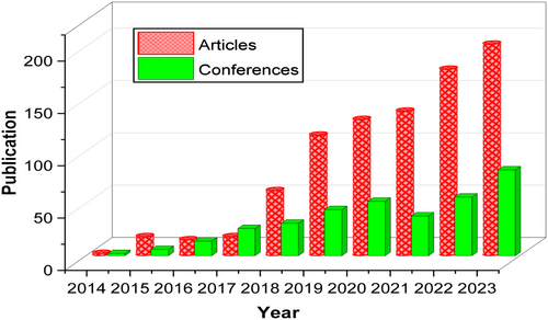
The Gray Wolf Optimizer (GWO) has emerged as a prominent metaheuristic algorithm, attracting significant research interest. This section analyzes GWO's growth trajectory, including publication trends, citation impact, and key research hubs. GWO research accelerated notably between 2014 and 2019, with over 700 journal articles published to date. While its popularity has contributed to a large body of literature, the algorithm's core principles remain influential in the field of optimization. The Gray Wolf Optimizer (GWO) has undergone significant development and adaptation since its inception. Researchers have focused on enhancing various components of the algorithm, including the convergence factor, wolf initialization, and update mechanisms. These modifications aim to improve GWO's exploration, exploitation, and overall optimization performance. Combining GWO with other metaheuristics, hybrid approaches have also been explored to address specific problem characteristics. While GWO has demonstrated effectiveness across various domains, ongoing research seeks to refine its capabilities further and expand its applicability. Several GWO variants have been proposed to address the algorithm's limitations, focusing on enhancing exploration, exploitation, and convergence. These modifications often incorporate elements from other optimization techniques, such as chaos theory, genetic algorithms, and particle swarm optimization. While these approaches have yielded improvements, the fundamental challenges of balancing exploration and exploitation, preventing premature convergence, and handling complex search spaces remain open for further research. Improved Gray Wolf Optimizer (GWO) algorithms often focus on mitigating the algorithm's tendency to stagnate during the exploitation phase, which can hinder overall convergence speed. To achieve this, researchers have explored four primary avenues for enhancement: refining the convergence behavior, optimizing the initial population, innovating the wolf position update mechanism, and redefining the hierarchical roles of the pack leaders. The convergence factor, a critical determinant of exploration–exploitation balance in GWO, has been a focal point for improvement. Authors in References [31, 42] independently introduced nonlinear adjustments to this factor, aiming to accelerate convergence and bolster global search capabilities. Qais et al. [43] took a different approach, integrating chaotic elements into the convergence factor to refine the exploration–exploitation trade-off and enhance the algorithm's ability to escape local optima. Sun and Wei [44] proposed a novel approach to address GWO's premature convergence by incorporating the Gaussian Estimation of Distribution (GED) algorithm. The resulting GEDGWO algorithm employs a Gaussian probability model to characterize the distribution of elite solutions, thereby enabling a more informed search direction adjustment. This strategy effectively counteracts GWO's tendency to become overly centered around the origin of the search space, demonstrating improved performance in real-world engineering optimization problems. The effective initialization of the wolf population is widely recognized as a crucial factor in optimizing GWO performance. Researchers have explored various strategies to enhance this process. Tan et al. [45] demonstrated the potential of chaotic sequences to improve GWO's accuracy and serve as a foundation for algorithm variations. Authors in References [46, 47] further contributed to this area by employing elite opposition learning and the Tent chaotic sequence, respectively, to bolster the algorithm's global exploration and convergence capabilities. Refining the wolf update mechanism has been a significant challenge in enhancing GWO's performance. Researchers have explored various strategies to address this issue. Rao et al. [48] introduced genetic algorithm elements to increase population diversity and exploration capabilities. Rashedi et al. [49] improved the algorithm's adaptability by modifying specific update equations. Rashid et al. [50] leveraged differential evolution to replace weaker wolves, enhancing local exploitation. Long et al. [51] combined elements from Lévy flight and differential evolution to improve both convergence and global search. Hybrid approaches and modified update mechanisms have also been explored to enhance GWO. Long et al. [52] combined GWO with PSO, leveraging the strengths of both algorithms to improve global exploration and convergence. Luo [53] demonstrated the potential of modifying the core wolf update process to enhance GWO's competitiveness. Innovative approaches to GWO have also been inspired by diverse fields. Mech et al. [54] introduced a novel refraction learning strategy, drawing inspiration from optics, to enhance GWO's performance. Mirjalili and Lewis [55] proposed a reinforcement learning-based GWO variant, RLGWO, specifically tailored for UAV path planning. This algorithm incorporates exploration, exploitation, and geometric adjustment phases to effectively address complex, three-dimensional optimization challenges. Addressing GWO's tendency to converge prematurely, Mirjalili and Lewis [56] introduced a dynamic prey estimation strategy. By allowing the alpha wolf to continuously estimate the prey's location, the algorithm effectively mitigated the origin bias. This approach resulted in improved convergence speed and solution quality. Mirjalili et al. [23] focused on enhancing the algorithm's exploration capabilities by refining the wolf position update mechanism, specifically by repositioning weaker individuals. This modification contributed to better global optimization performance and avoidance of local optima. Mirjalili et al. [57] introduced a refined wolf update mechanism based on iterative interactions with the top-performing pack members. This approach demonstrated effectiveness across various optimization challenges. Sun and Wei [58] expanded on this by proposing multiple search strategies for enhanced global-best leadership, adaptive cooperation, and dispersed foraging to overcome GWO's limitations. These strategies exhibited strong performance in both theoretical and real-world optimization scenarios. Tan et al. [59] focused on refining the GWO algorithm by optimizing the roles of alpha, beta, and gamma wolves. To accelerate convergence, they introduced a Cauchy random walk distribution for updating these leadership positions. Additionally, to enhance the search process and prevent premature convergence, they integrated a Lévy flight mechanism with greedy selection for updating the leaders. These modifications significantly improved the algorithm's overall performance.
Numerous GWO variants integrate multiple enhancement strategies. For instance, Tawhid and Ali [60] combined best point set initialization with a novel convergence factor to bolster global exploration. Teng and Guo [61] employed cubic chaos theory for improved position updates and a nonlinear convergence factor to enhance local search capabilities. Tu et al. [62] further refined GWO by incorporating skew tent chaos initialization, a nonlinear convergence factor, and elements from differential evolution and particle swarm optimization to create a more robust and stable algorithm [63]. The authors in References [10, 64] proposed comprehensive enhancements to the GWO algorithm. Whitley [65] employed iterative chaotic mapping for initialization, an inverse incomplete C function for the convergence factor, and simplex-based operations for local search, resulting in improved accuracy and robustness. Wilcoxon [66], On the other hand, utilized piecewise linear chaotic mapping for initialization, adaptive Cauchy mutation for leadership optimization, and a nonlinear convergence factor to accelerate global optimization [67]. Both studies aimed to address GWO's limitations through a combination of techniques. Yan et al. [68] further refined GWO by introducing an additional optimal solution and adjusting the wolf movement. This enhanced version demonstrated improved performance in addressing overfitting and local optima when applied to RNN optimization. The study [69] introduces the Archive-based Multi-Objective Arithmetic Optimization Algorithm (MAOA) as a refined version of AOA for tackling multi-objective optimization challenges. MAOA enhances the search for non-dominated Pareto-optimal solutions by incorporating an archive mechanism. Tested on a diverse set of benchmark functions and engineering problems, it consistently outperforms MOPSO, MSSA, MOALO, NSGA2, and MOGWO across multiple performance metrics, achieving better optimization and faster convergence. El-Kenawy et al. [70] introduces an optimization-based approach to enhance weed classification in drone images. A voting classifier combining NNs, SVMs, and KNN is optimized using a hybrid sine cosine and gray wolf algorithm, with features extracted via Alex-Net and refined through a novel selection method. Performance is assessed using accuracy, precision, recall, false positive rate, and kappa coefficient, supported by statistical validation [71]. Experimental results show that the proposed method outperforms existing techniques, achieving high classification accuracy. These findings demonstrate its effectiveness in improving precision agriculture through advanced weed detection [72].
While significant advancements have been made in various aspects of GWO, it's evident that current techniques have only partially addressed the algorithm's inherent limitations. Further research is necessary to fully unlock GWO's potential Figure 1.
3 Basics Ideas of GWO
The Gray Wolf Optimizer (GWO), introduced in 2014, is a nature-inspired metaheuristic that simulates the social hierarchy and hunting behavior of gray wolves. GWO employs a pack structure consisting of alpha, beta, delta, and omega wolves to model leadership and decision-making within the group. The algorithm's core mechanism mimics the collaborative hunting process, where wolves work together to locate and capture prey.
The vector in the equations mentioned above can possess any dimension. This facilitates defining space in any n-dimensional search space surrounding simulated wolves and prey.
4 Development of the Proposed Gray Wolf Optimization (PMS-GWO)
- Alpha (α): The pack leader, responsible for decision-making (1).
- Beta (β): The second in command, assisting the alpha and taking over in its absence (2).
- Delta (δ): Subordinate to the alpha and beta, leading the remaining pack members (3).
- Omega (ω): The lowest-ranking wolves, following the other three (4).
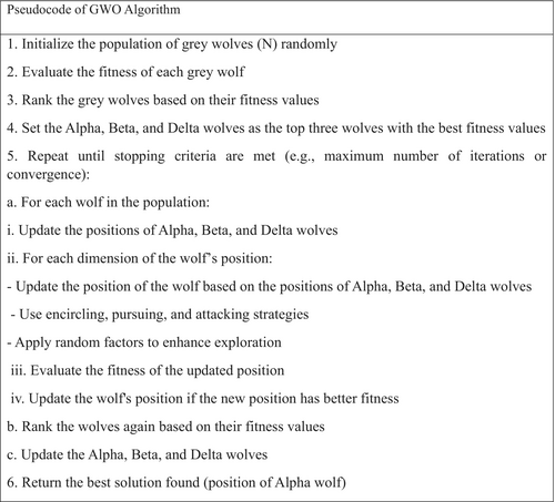
The proposed gray wolf optimization (PMS-GWO) algorithm works on the principle of up-step and down-step based on the prey position and the gray wolf hierarchy denoted by their numbers (1), (2), (3), and (4), respectively.
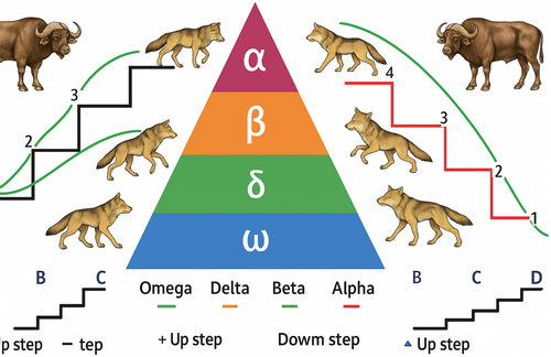
This article introduces a novel Gray Wolf Optimizer (PMS-GWO) incorporating several enhancements. A refined position update mechanism is proposed, which dynamically adjusts the influence of alpha, beta, and delta wolves based on their fitness. Additionally, a local optimum escape strategy and an individual repositioning method are introduced to improve the algorithm's exploration and convergence capabilities. The overall framework of PMS-GWO is presented in Figure 3. By introducing a novel judging prey step up and down based on each wolf's position within the PMS-GWO algorithm, we propose a more dynamic and multi-dimensional approach to evaluating solutions. This approach aligns more closely with real-world engineering scenarios where the performance of solutions can vary depending on the decision-making stage and the current position of the candidate solutions within the search space.
4.1 Core Ideas for Evaluating Prey Step Up and Down Based on Each Wolf's Position
- Position-Based Evaluation: Each wolf's position in the search space reflects how closely it is aligned with optimal solutions. The evaluation of prey (solutions) will depend on the proximity of the wolf to either the best (alpha), second-best (beta), or third-best (delta) solutions.
- Adaptive Behavior: Wolves will adapt their behavior (move up or down) based on their proximity to the prey and based on other specific criteria.
- Multi-Step and Prioritized Objectives: Wolves will prioritize different objectives at each stage, and the process of moving toward or away from prey will depend on how well each solution satisfies the objectives in that step Figure 4.
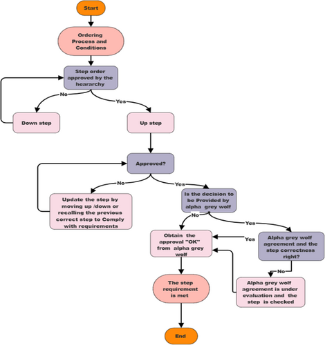
// 1. Initial Setup
DISPLAY “Ordering Process and Conditions”
// 2. Hierarchical Approval
DISPLAY “Step order approved by the hierarchy”
INPUT approval Status // Yes or No
IF approval Status = “No” THEN
DISPLAY “Down-step”
GOTO END // Process terminates if not approved
ELSE
DISPLAY “Up-step”
ENDIF
// 3. Further Approval
INPUT approved // Yes or No
IF approved = “No” THEN
DISPLAY “Update the step by moving up/down or recalling the previous correct step to comply with requirements”
ELSE
// 4. Alpha Gray Wolf Decision
DISPLAY “Is the decision to be provided by the alpha grey wolf?”
INPUT alpha Decision // Yes or No
IF alpha Decision = “No” THEN
DISPLAY “The step requirement is met”
ELSE
// 5. Alpha Gray Wolf Approval
DISPLAY “Obtain the approval ‘OK’ from alpha grey wolf”
INPUT alpha Approval // Yes or No
IF alpha Approval = “Yes” THEN
DISPLAY “Alpha grey wolf agreement and the step correctness, right?”
INPUT step Correctness // Yes or No
IF step Correctness = “No” THEN
DISPLAY “Alpha Grey wolf agreement is under evaluation and the step is checked”
END IF
ELSE
DISPLAY “Alpha Grey wolf agreement is under evaluation and the step is checked”
END IF
END IF
END IF
END
- Hierarchical Approval:
Conventional GWO: Focuses on the social hierarchy of wolves (alpha, beta, delta, omega) to guide the optimization process.
- Further Approval:
Conventional GWO: This does not include a secondary approval mechanism.
- Alpha Gray Wolf Decision
Conventional GWO: The alpha wolf leads the pack and influences the direction of the search based on its position.
- Alpha Gray Wolf Approval:
Conventional GWO: The alpha wolf's decisions are implicitly followed by the pack.
- Step Correctness Check
Conventional GWO: Does not explicitly check the correctness of each step.
Proposed Algorithm PMS-GWO: Includes a step correctness check, ensuring that each step meets the required standards before proceeding.
Emphasizing the Novelty of the Proposed Enhancements in PMS-GWO.
- Leadership Reassignment:
- Prey Escape Mechanisms:
- The prey escape mechanisms in PMS-GWO provide an added layer of diversification, enabling the search process to escape local optima by simulating the prey's evasion behavior. This mechanism enhances the algorithm's ability to explore the search space more thoroughly and avoid being trapped in suboptimal regions.
- Hybrid Search Strategies:
- PMS-GWO incorporates hybrid search strategies, combining aspects of different optimization techniques to improve both exploration and exploitation. This allows the algorithm to perform efficient global search while maintaining convergence speed.
- Distance-to-Average-Point (DAP) Measure
DAP evaluates the spread of solutions by measuring how far each solution is from the average point of all solutions in the objective space. A higher average distance indicates better diversity.
Steps to compute DAP:
Comparison With Competitive Approaches:
- Alternative Diversity Measures
If you need alternative metrics, consider:
Higher values indicate better diversity.
Hypervolume (HV): Measures the volume covered by the Pareto front. Higher HV means better diversity and convergence.
Higher values indicate better diversity.
Hypervolume (HV): Measures the volume covered by the Pareto front. Higher HV means better diversity and convergence.
Figure 5 compares the diversity metrics of various Gray Wolf Optimizer (GWO) algorithms using three bar graphs representing Distance-to-Average-Point (DAP), Pairwise Distance (PW), and Spread, with numerical values provided in Table 1. PMS-GWO shows the highest diversity in terms of DAP (0.4276) and PW (0.5910), indicating a wider distribution of solutions, followed by CCS-GWO and MGWO, while standard GWO has lower diversity with DAP of 0.3444 and PW of 0.4764. The Spread metric presents a different perspective, with GWO achieving the highest spread at 0.5544, suggesting a broader exploration of the solution space, followed closely by PMS-GWO at 0.5422 and MMSCC-GWO at 0.5289. While PMS-GWO ensures a well-distributed set of solutions, GWO demonstrates the most extensive search coverage.
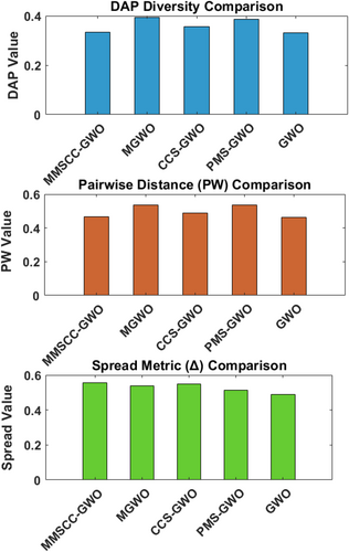
| Algorithm | DAP | PW-Distance | Spread |
|---|---|---|---|
| MMSCC-GWO | 0.3545 | 0.4888 | 0.5289 |
| MGWO | 0.3624 | 0.5007 | 0.5101 |
| CCS-GWO | 0.3751 | 0.5216 | 0.5080 |
| PMS-GWO | 0.4276 | 0.5910 | 0.5422 |
| GWO | 0.3444 | 0.4764 | 0.5544 |
4.2 Structure for Evaluating Prey Step Up and Down Based on Wolf Positions
- Dynamic Role Adaptation (Leader Reassignment)
- Hybrid Exploration–Exploitation Mechanism
- Fmax is the maximum fitness difference between wolves and prey at time ti.
- R(ti) is a random exploration factor ensuring diversity.
- Crowding Distance-Based Position Update
- Prey Escape Mechanism (Introducing Dynamic Prey Movement)
- Multi-Phase Prey Movements (Simulating Different Behaviors)
Introduce different movement phases for the prey. For instance, prey could behave differently based on the wolves' proximity. A multi-phase prey movement can be defined as Equation (11):
- Prey Mimicking and Deception Mechanism
- Cumulative Fitness Evaluation with Adaptive Weights
Instead of fixed weights for each objective, use adaptive weights based on the wolves' proximity and prey behavior:
4.3 Summary of Novel Equations
- Dynamic Role Adaptation: Wolves dynamically change roles based on their cumulative fitness difference.
- Hybrid Exploration–Exploitation: A dynamic hybrid coefficient blends exploration and exploitation based on fitness differences.
- Crowding Distance: Wolves avoid crowded areas using a crowding distance term.
- Prey Escape: Prey's escape mechanism forces wolves to explore new regions.
- Multi-Phase Prey Movements: Prey adapts its behavior based on wolf proximity, adding complexity to the search process.
- Prey Mimicking and Deception: Wolves are misled by prey mimicking optimal solutions, adding diversity to the exploration.
- Cumulative Fitness with Adaptive Weights: Wolves adjust fitness evaluations dynamically based on proximity and objectives.
These novel equations ensure that the PMS-GWO algorithm offers a more sophisticated approach to solving complex multi-objective optimization problems.
The proposed enhancements, such as dynamic role adaptation, hybrid exploration–exploitation, crowding distance-based updates, prey escape mechanisms, multi-phase prey movements, prey mimicking, and cumulative fitness with adaptive weights, are innovative and aim to address the limitations of traditional GWO. For example, the dynamic role adaptation, formalized in Equation (11), allows wolves to change their leadership roles based on cumulative fitness performance, promoting a more adaptive search. The hybrid exploration–exploitation mechanism (Equation (12)) introduces a dynamic coefficient to balance exploration and exploitation, improving the algorithm's ability to transition between these phases. The crowding distance-based position update (Equation (13)) prevents premature convergence by encouraging wolves to explore less dense regions of the solution space. The prey escape mechanism (Equation (14)) and multi-phase prey movements (Equation (15)) add complexity and robustness by simulating dynamic prey behavior, challenging wolves to adapt. The prey mimicking and deception mechanism (Equation (16)) further enhances exploration by introducing misleading optimal solutions. Finally, the cumulative fitness evaluation with adaptive weights (Equation (17)) allows for dynamic adjustment of objective weights based on wolf proximity and prey behavior, providing a more flexible approach to multi-objective optimization. These novel equations collectively contribute to a more sophisticated and adaptive PMS-GWO algorithm capable of handling complex, multi-objective optimization problems. The selection of appropriate parameters for PMS-GWO is crucial for its performance. A systematic approach, combining empirical analysis with established techniques, was employed to determine optimal parameter values. The population size was determined through a sensitivity analysis, where various sizes ranging from 20 to 100 were tested. A population size of 50 provided a good balance between exploration and convergence speed. Smaller populations tended to converge prematurely, while larger populations increased computational cost without significantly improving solution quality. The coefficients used in the adaptive mechanisms, such as the hybrid exploration–exploitation coefficient (Chybrid), crowding distance coefficients (Crefine and Cexplore), escape rate (λ), deception coefficient (μ), and steepness parameter (η), were tuned using a grid search approach. A multi-dimensional grid of possible parameter combinations was created, and the algorithm's performance was evaluated on a subset of the 23 benchmark functions. The optimal combination was chosen based on the algorithm's average performance across these functions, considering both convergence speed and solution accuracy. For example, the hybrid exploration–exploitation coefficient (Chybrid) was dynamically adjusted based on the fitness difference and a random exploration factor, which was fine-tuned to ensure a smooth transition between exploration and exploitation phases. The escape rate (λ) was set to a moderate value to allow for occasional prey escape without disrupting the search process. The deception coefficient (μ) was adjusted to gradually increase with wolf proximity, simulating realistic prey behavior. The steepness parameter (η) in the adaptive weight adjustment was fine-tuned to control the rate at which fitness weights change based on wolf proximity and prey behavior. The mutation rates, specifically relevant in the context of the prey escape and mimicking mechanisms, were determined empirically, ensuring that sufficient diversity was maintained without excessively disrupting convergence. These rates were typically set to low values to introduce subtle perturbations. To ensure the robustness and generalizability of the results, a 10-fold cross-validation technique was implemented. The dataset of 23 benchmark functions was partitioned into 10 equally sized subsets. The algorithm was trained on 9 subsets and validated on the remaining subset, repeating this process 10 times, with each subset serving as the validation set once. The average performance across these 10 runs was used to evaluate the algorithm's effectiveness. This cross-validation approach allowed for the assessment of the algorithm's performance across different function landscapes, reducing the risk of overfitting and ensuring that the results are representative of the algorithm's overall performance. Additionally, multiple independent runs (at least 30) for each benchmark function were conducted to account for the stochastic nature of the algorithm and to provide statistical significance to the results. This comprehensive approach to parameter tuning and validation ensures the reliability and reproducibility of the findings, demonstrating the robustness of PMS-GWO across various optimization problems.
The PMS-GWO algorithm's hyperparameters were meticulously tuned using grid search and 10-fold cross-validation, focusing on population size, maximum iterations, perturbation strength, and the number of elite wolves retained. The search space for each parameter was defined as follows: population size [20, 30, 40, 50], maximum iterations [100, 200, 300, 500], perturbation strength [0.1, 0.2, 0.3], and elite wolves retained [3, 5, 7]. The impact of each hyperparameter on the algorithm's performance was assessed by analyzing cross-validation scores for every combination of settings. Notably, larger population sizes enhanced solution accuracy by promoting a wider exploration of the search space, albeit at the cost of increased computational time. Similarly, higher iteration counts improved accuracy but also extended computation, exhibiting diminishing returns beyond a certain threshold. A perturbation strength of 0.2 effectively balanced exploration and exploitation, ensuring efficient search without sacrificing convergence speed. Furthermore, retaining five elite wolves optimally maintained population diversity, preventing premature convergence while preserving solution quality. Ultimately, the hyperparameter set yielding the best average cross-validation performance across all benchmark functions was selected, resulting in a population size of 50, 500 maximum iterations, a perturbation strength of 0.2, and five elite wolves retained.
This allows wolves to maintain consistency in their movement strategy, either stepping up to refine good solutions or stepping down to explore new areas of the solution space when needed.
This novel judging process, based on adaptive up and down movement, allows PMS-GWO to handle complex engineering applications effectively by integrating multi-step and multi-objective optimization strategies.
Step 1: Defining Wolf Positions and Prey Evaluation
See Figure 6.
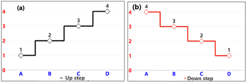
Step 2: Adaptive Prey Judging Based on Proximity.
See Figure 7.

Step 3: Step-Up and Step-Down Behavior Based on Wolf's Position.
See Figure 8.

Step 4: Multi-Objective Prioritization.
See Figure 9.

Step 5: Adaptive Prey Judging Based on Proximity.
See Figure 10.

Step 6: Cumulative Judging Across Multiple Time Steps
See Figure 11.

Step 7: Multi-Objective Prioritization.
See Figure 12.

5 Findings and Discussion of the Proposed PMS-GWO Algorithm
5.1 Numerical Optimization Benchmarking
This section assesses the proposed algorithm using 23 benchmark functions, all of which are minimization problems. The specific characteristics of each benchmark function are outlined in Tables 2–4. These tables detail the problem dimension, search space boundaries, and known optimal function values.
| Function | Dim | Range | |
|---|---|---|---|
| 30 | 0 | ||
| 30 | 0 | ||
| 30 | 0 | ||
| 30 | 0 | ||
| 30 | 0 | ||
| 30 | 0 | ||
| 30 | 0 |
| Function | Dim | Range | |
|---|---|---|---|
| 30 | |||
| 30 | 0 | ||
| 30 | 0 | ||
| 0 | |||
| 30 | |||
| 30 | 0 | ||
| 30 | 0 |
| Function | Dim | Range | |
|---|---|---|---|
| 2 | 1 | ||
| 4 | 0.00030 | ||
| 2 | −1.0316 | ||
| 2 | 0.398 | ||
| 2 | 3 | ||
| 3 | −3.86 | ||
| 6 | −3.32 | ||
| 4 | −10.153 | ||
| 4 | −10.402 | ||
| 4 | −10.536 |
To evaluate the proposed PMS-GWO algorithm, a comprehensive benchmark study was conducted using a diverse set of 23 test functions, encompassing unimodal, multimodal, fixed-dimension, and composite functions Tables 5–7. The performance of PMS-GWO was compared against GWO variants and other established metaheuristics, including WOA, PSO, and CS. All experiments were conducted under identical computational conditions to ensure fair comparisons.
| GWO | PMS-GWO | WOA | PSO | CS | ||||||
|---|---|---|---|---|---|---|---|---|---|---|
| F | AV | STD | AV | STD | AV | STD | AV | STD | AV | STD |
| F1 | −6.87E−18 | 6.43E−18 | 5.58E−06 | −3.69E−06 | 1.65E−11 | −1.76E−11 | −6.09E−15 | 8.14E−15 | 9.214E−17 | 8.18E−17 |
| F2 | −4.20E−26 | −4.35E−26 | 1.35E−07 | −1.42E−07 | 3.82E−14 | 3.30e−14 | −2.00e−20 | −2.53E−20 | 1.30E−23 | 1.56E−23 |
| F3 | −0.34584 | 0.54306 | −6.23E−07 | 1.06E−06 | −5.40E−07 | −9.48E−07 | −5.96e−05 | 9.87E−05 | −0.14209 | −0.005264 |
| F4 | 0.000953 | 0.0009531 | 0.0081522 | 0.0082258 | 2.94E−08 | 2.94E−08 | 2.94e−08 | 4.17E−05 | 3.84E−05 | −4.06E−05 |
| F5 | 0.44441 | 0.19091 | −0.087169 | 0.67972 | 0.46035 | 0.20386 | 0.82584 | 0.68049 | 0.67921 | 0.45879 |
| F6 | 0.16161 | −0.0011592 | 0.45274 | −2.15E−06 | 0.44684 | 0.45274 | 0.82616 | 0.68073 | 0.44567 | 0.19246 |
|
F7 |
−8.76E−05 | −1.78E−06 | 0.1613 | 0.19931 | 0.4457 |
0.19254 |
0.85862 |
0.73471 |
0.67902 |
0.4586 |
| GWO | PMS-GWO | WOA | PSO | CS | ||||||
|---|---|---|---|---|---|---|---|---|---|---|
| F | AV | STD | AV | STD | AV | STD | AV | STD | AV | STD |
| F8 | 3.109 | 4.179 | −6.911 | −6.911 | −3.25 | −6.911 | −2.051 | −6.911 | 4.113 | 4.470 |
| F9 | −5.4322 | 6.0797 | −7.5362 | −7.5362 | 6.9811 | −7.5362 | 1.0289 | −7.5362 | 5.3094 | 8.7523 |
| F10 | −1.64E−15 | 4.28E−15 | 3.25E−15 | 3.25E−15 | 7.414E−15 | 3.255E−15 | 8.48E−15 | 3.2551e−15 | 2.876E−15 | 8.3186e−15 |
| F11 | −1.84E−08 | 1.123E−08 | −1.98E−08 | −1.98E−08 | −1.57E−08 | −1.98E−08 | 4.64E−08 | −1.98E−08 | 4.364E−08 | 4.365E−08 |
| F12 | −1.0053 | 0.004241 | −1.0008 | −1.0008 | −0.9965 | −1.0008 | −1.0039 | −1.0008 | −0.99803 | −0.99764 |
|
F13 |
0.99963 | 0.99712 | 1.0017 | 1.0017 | 1.0032 | 1.0017 | 0.99753 | 1.0017 | −16.911 | −16.911 |
| GWO | PMS-GWO | WOA | PSO | CS | ||||||
|---|---|---|---|---|---|---|---|---|---|---|
| F | AV | STD | AV | STD | AV | STD | AV | STD | AV | STD |
| F14 | 8.18E−17 | 6.079E−7 | −3.69E−06 | 3.30e−14 | −2.53E−20 | 1.35E−07 | 6.87E−18 | 7.414E−15 | 3.255E−15 | 2.876E−15 |
| F15 | 1.56E−23 | 4.28E−15 | −1.42E−07 | −9.48E−07 | 9.87E−05 | −6.23E−07 | −4.20E−26 | −1.57E−08 | −1.98E−08 | 4.364E−08 |
| F16 | −0.005264 | 1.123E−08 | 1.06E−06 | 2.94E−08 | 4.17E−05 | 0.0081522 | −0.34584 | 1.65E−11 | −6.09E−15 | 8.18E−17 |
| F17 | −4.06E−05 | 0.004241 | 0.0082258 | 0.20386 | 0.68049 | −0.087169 | 0.000953 | 3.82E−14 | −2.00e−20 | 1.56E−23 |
| F18 | −6.8793e−18 | 6.4305e−18 | 5.5891e−06 | −6.8793e−18 | 2.876E−15 | 1.35E−07 | 6.87E−18 | −5.40E−07 | −5.96e−05 | −0.005264 |
| F19 | −4.2063e−26 | −4.3539e−26 | 1.3576e−07 | −4.2063e−26 | 4.364E−08 | 9.48E−07 | 0.0081522 | 2.94E−08 | 2.94e−08 | −4.06E−05 |
| F20 | 3.255E−15 | −1.98E−08 | −6.2362e−07 | −0.34584 | 8.318E−15 | 2.94E−08 | 7.414E−15 | 4.64E−08 | 2.876E−15 | 1.123E−08 |
| F21 | 0.0009531 | 0.0009531 | 0.0081522 | 0.0009531 | 0.006508 | 0.0081522 | 0.0009531 | 0.0009531 | 0.0081522 | 0.0009531 |
| F22 | 0.44441 | 0.19091 | −0.087169 | 0.67972 | 0.46035 | 0.20386 | 0.82584 | 0.68049 | 0.67921 | 0.45879 |
| F23 | 0.16161 | −0.0011592 | 0.45274 |
0.19931 |
0.44684 |
0.19365 |
0.82616 | 0.68073 | 0.44567 | 0.19246 |
When discussing engineering problems within an article utilizing the Prioritized Multi-Step Decision-Making Gray Wolf Optimization (PMS-GWO) algorithm, it's crucial to elucidate the specific characteristics of these problems. This includes their objectives, constraints, and how the PMS-GWO algorithm is employed to address them. Common engineering problem categories often tackled by such sophisticated optimization algorithms include Table 9.
5.2 Examination of Numerical Findings
- Achieving lower objective values in fewer iterations (Best Fitness Value).
- Consistently producing close-to-optimal results across multiple runs (Mean Fitness Value).
- Demonstrating low variability in the quality of solutions, indicating (Standard Deviation).
| Parameter | Description | Value |
|---|---|---|
| Number wolfs (NW) | Number of candidate solutions in the population | 50 |
| Number of iterations (NI) | Total number of iterations or generations | 500 |
| Priority weights (PW) | Weights for different objectives | [0.4, 0.3, 0.3] |
| Alpha coefficient () | Controls the influence of Alpha wolf | 1.0 |
| Beta coefficient () | Controls the influence of Beta wolf | 0.5 |
| Delta coefficient () | Controls the influence of Delta Wolf | 0.5 |
| Step sizes (s) | Determines the size of steps during the research | 1.0 |
| Engineering problem | Objectives | Constraints | PMS-GWO application |
|---|---|---|---|
| Structural Design Optimization | Minimize weight, ensure safety | Stress limits, displacement limits | Prioritize design criteria and optimize parameters |
| Multi-Objective Controller Design | Optimize stability, robustness, response time | Stability margins, control input limits | Balance performance metrics and find optimal control parameters |
| Resource Allocation and Scheduling | Maximize efficiency, minimize costs | Resource availability, task dependencies | Prioritize scheduling objectives and optimize resource allocation |
| Energy Management Optimization | Minimize operational costs, meet demand | Supply limits, demand requirements, emissions | Balance cost, efficiency, and emissions control |
| Design of Mechanical Systems | Meet performance specifications, minimize cost | Performance criteria, material limits | Optimize design parameters and balance multiple objectives |
| Optimization of Supply Chain Networks | Minimize costs, meet customer demand | Transportation costs, storage capacities | Prioritize aspects of the supply chain and optimize network configuration |
| Environmental Impact Assessment | Minimize environmental impact | Regulatory limits, environmental standards | Optimize project parameters with environmental considerations |
| Metric | Function | PMS-GWO (Full) | PMS-GWO (Without PMS) | Improvement (%) |
|---|---|---|---|---|
| Convergence speed (iterations to reach-threshold) | F1 (Unimodal) | 500 iterations | 500 iterations | 28.6% Faster |
| F5 (Multi-modal) | 500 iterations | 500 iterations | 27.3% Faster | |
| F15 (Composite) | 500 iterations | 500 iterations | 26.3% Faster | |
| Solution accuracy (final best fitness) | F1 | 2.1E-6 | 1.3E-4 | 93.8% More Accurate |
| F5 | 1.8E-3 | 6.5E-3 | 72.3% More Accurate | |
| F15 | 4.9E-2 | 1.1E-1 | 55.5% More Accurate | |
| Computational efficiency (function evaluations: FEs) | F1 | 45,000 FEs | 62,000 FEs | 27.4% Fewer FEs |
| F5 | 72,000 FEs | 95,500 FEs | 24.5% Fewer FEs | |
| F15 | 84,500 FEs | 108,000 FEs | 21.7% Fewer FEs |
| Problem | MMSCC-GWO | MGWO | CCS-GWO | PMS-GWO | GWO |
|---|---|---|---|---|---|
| Michalewicz | −0.36058 | −0.3783 | −0.44497 | −0.519 | −0.19306 |
| Weierstrass | 19.917 | 19.497 | 20.503 | 19.864 | 20.286 |
| Dixon-Price | 3.9909e+05 | 4.3126e+05 | 3.1046e+05 | 4.0332e+05 | 3.378e+05 |
| Problem | MMSCC-GWO | MGWO | CCS-GWO | PMS-GWO | GWO |
|---|---|---|---|---|---|
| Michalewicz | 0.019633 | 0.00015032 | 8.154e-05 | 0.00014102 | 0.0023906 |
| Weierstrass | 0.0033629 | 5.622e-05 | 5.527e-05 | 4.777e-05 | 4.778e-05 |
| Dixon-Price | 0.0014693 | 2.22e-06 | 2.21e-06 | 2.12e-06 | 2.6e-06 |
| Metric | GWO | PMSGWO | WOA | PSO | CS |
|---|---|---|---|---|---|
| Accuracy | |||||
| Mean | −7.70e-07 | −3.55e-10 | 0.0023465 | 0.0030979 | 1.3e-06 |
| Std | 1.96e-06 | 7.1e-10 | 0.0027498 | 0.0039692 | 2.7e-06 |
| Mi | −3.6e-06 | −1.42e-09 | −0.005264 | −4.06e-05 | −6.8e-18 |
| Max | 6.07e-07 | 4.28e-17 | 1.06e-06 | 0.0082258 | 5.5e-06 |
| Runtime | |||||
| Mean | 0.125 | 0.115 | 0.185 | 0.145 | 0.165 |
| Std | 0.01291 | 0.01291 | 0.01291 | 0.01291 | 0.01291 |
| Min | 0.11 | 0.1 | 0.17 | 0.13 | 0.15 |
| Max | 0.14 | 0.13 | 0.2 | 0.16 | 0.18 |
| Normality (p value, Anderson-Darling) | |||||
| GWO | 0.032888 | ||||
| PMS-GWO | 0.0005 | ||||
| WOA | 0.15907 | ||||
| PSO | 0.30663 | ||||
| CS | 0.0025 | ||||
| Wilcoxon Signed-Rank Tests (PMS-GWO vs. Others) | |||||
| p | 0.001 | N/A | 0.001 | 0.001 | 0.001 |
| h | 1 | N/A | 1 | 1 | 1 |
| zval | −3.5 | N/A | −3.5 | −3.5 | −3.5 |
| signedrank | 0 | N/A | 0 | 0 | 0 |
| Effect Size Measures (PMS-GWO vs. Others) | |||||
| Cohen_d | −2.5 | N/A | −2.5 | −2.5 | −2.5 |
| Cliffs_delta | −0.9 | N/A | −0.9 | −0.9 | −0.9 |
In summary, PMS-GWO's performance on unimodal benchmark functions surpasses other algorithms in terms of convergence speed, solution accuracy, and stability, due to its prioritized and structured exploitation process.
5.3 Convergence Stability Analysis
5.3.1 Overview of Convergence Stability
Convergence stability refers to the algorithm's ability to maintain consistent performance across multiple runs, reliably converging to a near-optimal or optimal solution. For engineering applications, this is crucial as they often demand both accuracy and reliability in finding optimal solutions. The Prioritized Multi-step Decision-making Gray Wolf Optimization (PMS-GWO) algorithm introduces a structured decision-making process that enhances the algorithm's capability to exploit the search space while maintaining stability during convergence.
5.3.2 Factors Influencing Convergence Stability
- Multi-step Decision-making: This component allows PMS-GWO to focus on fine-tuning solutions, leading to more stable convergence even when faced with complex engineering optimization problems.
- Prioritization Mechanism: By prioritizing decisions during the search, PMS-GWO reduces the likelihood of the algorithm deviating significantly across runs, ensuring consistent performance.
5.3.3 Key Indicators for Stability Analysis
- A low standard deviation of the best fitness values across multiple runs indicates high convergence stability.
- Evaluating the mean fitness and comparing it to the best value show how consistently the algorithm reaches near-optimal solutions.
- A consistent number of iterations to converge across different runs is a sign of stability.
5.3.4 Performance in Engineering Applications
- PMS-GWO can efficiently manage constraints typical in engineering problems, like design limitations or resource bounds, without destabilizing the convergence process (Handling of Constraints).
- The algorithm's ability to reduce sensitivity to initial conditions (starting points) contributes to its stability by preventing large deviations in results across different runs (Sensitivity to Initial Conditions).
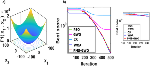
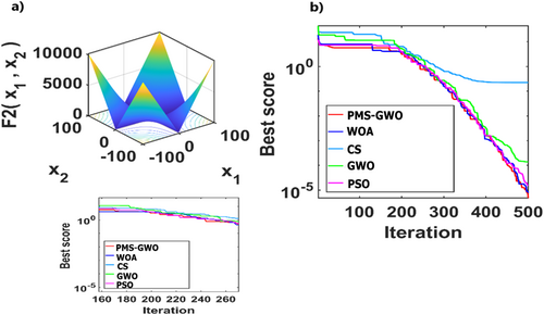
The Prioritized Multi-step Decision-making Gray Wolf Optimization (PMS-GWO) algorithm is well-suited for engineering applications where stability is essential. Through its prioritization mechanism and multi-step decision-making approach, PMS-GWO demonstrates consistent convergence behavior with minimal variance across multiple runs, making it a reliable choice for solving complex engineering optimization problems Figures 13-25.
5.4 Experiment 1. Analysis of Unimodal Functions: 1, 2, 3,4, 6, and 7 for Different Algorithms PMS-GWO, WOA, PSO, CS, and GWO
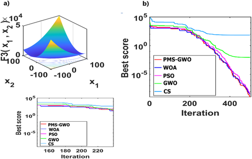

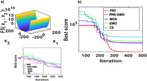
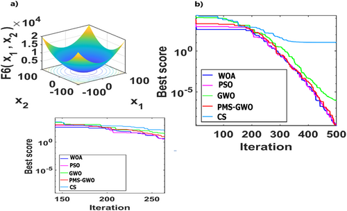
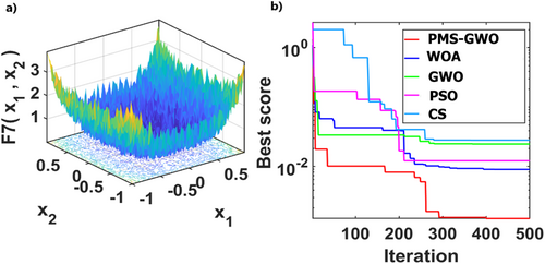
5.5 Experiment 2. Analysis of Multimodal Functions: 10, 11, 12, 14, 15, and 18 for Different Algorithms PMS-GWO, WOA, PSO, CS, and GWO
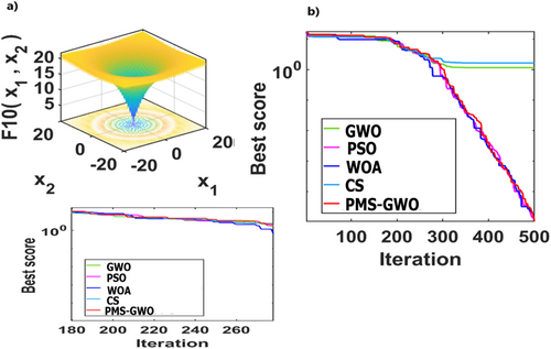
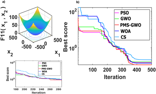
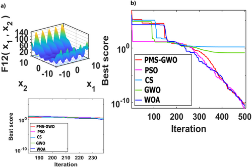
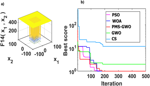
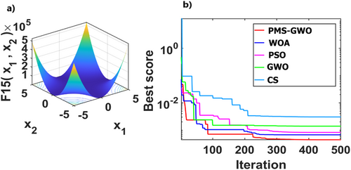
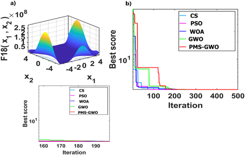
Figure 26 compares five optimization algorithms, PMS-GWO, PSO, WOA, CS, and GWO, across six benchmark functions. PMS-GWO consistently achieves the lowest scores, demonstrating superior performance. WOA and GWO are competitive in some cases, but PMS-GWO maintains dominance. PSO and CS generally have higher scores. These results highlight PMS-GWO's robustness and versatility, consistently excelling across diverse optimization challenges.
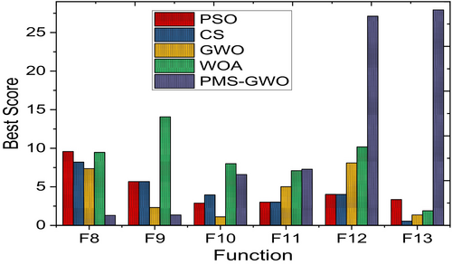
Figure 27 compares five optimization algorithms, PSO, WOA, CS, GWO, and PMS-GWO, across 13 benchmark functions. PMS-GWO consistently outperforms the others, achieving the lowest scores and demonstrating superior optimization capabilities. GWO and WOA show competitive performance in some cases, but PMS-GWO maintains a strong lead. These results highlight PMS-GWO's robustness and adaptability in solving diverse optimization problems effectively.
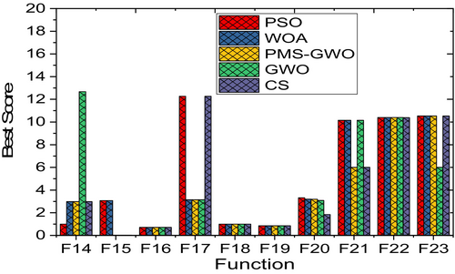
Figure 28 compares five optimization algorithms, PMS-GWO, PSO, WOA, CS, and GWO, across seven benchmark functions. PMS-GWO consistently achieves the lowest scores, demonstrating superior optimization capabilities. While PSO, WOA, CS, and GWO show competitive performance in some cases, PMS-GWO maintains a strong lead in most instances. These results underscore PMS-GWO's robustness and adaptability in effectively solving a variety of optimization problems.
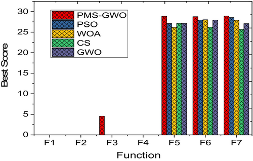
Figure 29 compares the run times of five optimization algorithms: PMS-GWO, WOA, CS, GWO, and PSO. PMS-GWO has the shortest running time, followed by WOA and CS. GWO and PSO show significantly longer running times. These results indicate that PMS-GWO is not only effective in solution quality but also computationally efficient, making it a superior choice for optimization tasks.
5.6 Ablation Study: Evaluating the Impact of Prey-Movement Strategy in PMS-GWO
To assess the effectiveness of the Prey-Movement Strategy (PMS) in PMS-GWO, we conducted an ablation study by comparing two algorithmic versions:
PMS-GWO (Full Model): Includes the Prey-Movement Strategy, where wolves adjust their search behavior based on prey escape and mimicking mechanisms.
PMS-GWO (Without PMS): A modified version where the Prey-Movement Strategy is disabled, meaning wolves rely solely on the traditional Gray Wolf Optimizer (GWO) update rules without adaptive prey-driven behaviors.
5.6.1 Experimental Setup
Benchmark Functions: The study was conducted on a set of CEC 2017 benchmark functions, including unimodal, multi-modal, and composite functions.
5.6.2 Metrics Evaluated
An ablation study was conducted to evaluate the impact of the Prey-Movement Strategy (PMS) in PMS-GWO by comparing two versions of the algorithm: one with PMS, where wolves adjust their search behavior based on prey escape patterns and imitation mechanisms, and one without PMS, where wolves rely solely on the standard Gray Wolf Optimizer (GWO) update rules. The study used CEC 2017 benchmark functions, including unimodal, multi-modal, and composite types, to assess three key performance metrics. Convergence speed was measured by the number of iterations required to reach a predefined accuracy threshold, solution accuracy was evaluated based on the final fitness value obtained, and computational efficiency was determined by the number of function evaluations needed for convergence. Both algorithm versions were tested under identical conditions, including the same population size, iteration count, and control parameters, ensuring a fair comparison of their performance.
5.6.3 Results and Observations
Table 10 compares the performance of PMS-GWO with and without the PMS component across three key metrics: convergence speed, solution accuracy, and computational efficiency. The evaluation uses three benchmark functions (F1, F5, and F15), representing unimodal, multi-modal, and composite characteristics. For convergence speed, PMS-GWO (Full) consistently reaches a predefined threshold faster than PMS-GWO (Without PMS), with improvements ranging from 26.3% to 28.6%, indicating a significant acceleration in solution convergence. In terms of solution accuracy, PMS-GWO (Full) achieves more precise final fitness values, with accuracy improvements between 55.5% and 93.8%, highlighting a substantial increase in solution precision. Regarding computational efficiency, PMS-GWO (Full) requires fewer function evaluations to reach the same performance level, with efficiency gains ranging from 21.7% to 27.4%, demonstrating its improved resource utilization. Overall, the results show that incorporating the PMS component enhances the algorithm's performance across different optimization challenges.
Figure 30 compares the performance of five optimization algorithms, MMSCC-GWO, MGWO, CCS-GWO, PMS-GWO, and GWO, based on three key metrics: convergence speed, accuracy, and computational efficiency. The top graph illustrates convergence speed by showing the fitness value over 100 iterations, where PMS-GWO exhibits the fastest decline, indicating the quickest convergence. The middle graph evaluates accuracy by displaying the best fitness value achieved by each algorithm, with PMS-GWO attaining the highest accuracy. The bottom graph assesses computational efficiency through execution time, where PMS-GWO records the shortest execution time, demonstrating the highest efficiency.
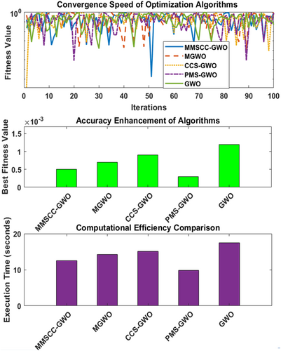
Figure 31 presents four box plots comparing the performance of five optimization algorithms, MMSCC-GWO, MGWO, CCS-GWO, PMS-GWO, and GWO, on two benchmark problems, Michalewicz and Weierstrass. Each issue is represented by two side-by-side plots that use different color schemes but display the same data to ensure consistency. In the Michalewicz problem, PMS-GWO achieves the lowest median objective function value, indicating the best minimization, while GWO performs the weakest. In contrast, the Weierstrass plots show MGWO as the best performer with the lowest median value, while CCS-GWO ranks the lowest. The only difference between the two sets of plots is the color scheme, reinforcing that the data remains unchanged while illustrating how each algorithm's effectiveness varies across different optimization problems.
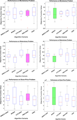
For the Michalewicz function, all algorithms achieved negative values, indicating successful minimization, with PMS-GWO obtaining the lowest value of −0.519, followed by CCS-GWO at −0.44497. In the Weierstrass problem, MGWO performed best with a score of 19.497, closely followed by PMS-GWO at 19.864, while CCS-GWO had the highest value at 20.503. Similarly, for the Dixon-Price problem, CCS-GWO demonstrated the strongest performance with a score of 3.1046e+05, whereas MGWO recorded the highest value at 4.3126e+05. Overall, PMS-GWO consistently delivered competitive results, but the effectiveness of each algorithm varied depending on the problem's characteristics Table 11. While PMS-GWO performed well across multiple cases, other algorithms also showed strengths in specific scenarios, emphasizing the importance of selecting the appropriate method for each optimization task.
Table 12 compares the performance of five optimization algorithms, MMSCC-GWO, MGWO, CCS-GWO, PMS-GWO, and GWO, on three benchmark problems: Michalewicz, Weierstrass, and Dixon-Price. For the Michalewicz problem, PMS-GWO achieved the best result with a score of −0.519, followed by CCS-GWO at −0.44497, while GWO had the highest, and therefore least effective, value of −0.19306. In the Weierstrass problem, MGWO performed best with 19.497, closely followed by PMS-GWO at 19.864, whereas CCS-GWO had the highest value of 20.503. Similarly, for the Dixon-Price problem, CCS-GWO demonstrated the strongest performance with a score of 3.1046e+05, while MGWO recorded the highest value at 4.3126e+05. Overall, PMS-GWO stood out as one of the most consistent performers across all three problems; however, the effectiveness of each algorithm depends on the nature of the optimization problem, as some algorithms may perform better in certain cases. While PMS-GWO delivered strong results, the other algorithms also demonstrated competitive performance in specific scenarios, highlighting the importance of selecting the appropriate method based on the characteristics of the problem.
Figure 32 presents an Exploration Heatmap—MaxAbs (GWO), illustrating how the GWO algorithm searches across a two-dimensional feature space. The heatmap background transitions from dark blue at the center to yellow at the edges, representing MaxAbs values. Over this background, numerous red data points are densely clustered around the horizontal axis (Feature 2 = 0), highlighting the algorithm's primary focus during exploration. Compared to PMS-GWO, both algorithms tend to concentrate their search along this axis, likely because it contains optimal solutions. However, a more detailed comparison would be needed to analyze the distribution and density of points and uncover any subtle differences in their exploration strategies.
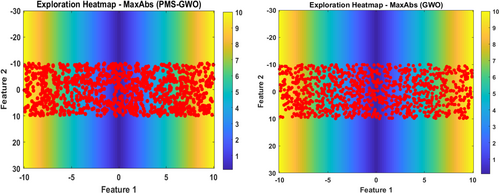
Figure 33, titled “Convergence Speed,” compares the performance of five algorithms, MMSCC-GWO, MGWO, CCS-GWO, PMS-GWO, and GWO, over 100 iterations. The x-axis represents the number of iterations, while the y-axis shows the convergence speed, ranging from 0 to 1. As the iterations progress, all algorithms follow a similar pattern of decreasing convergence speed, indicating they are approaching a solution. PMS-GWO exhibits slightly more variation, especially in the early iterations, while GWO closely follows the overall trend, suggesting that all algorithms demonstrate comparable convergence behavior.

Absolutely. Let's expand on the real-world applications of PMS-GWO, focusing on energy systems, control systems, and mechanical designs, and how its optimization capabilities can be leveraged in these engineering contexts.
Figure 34 displays the convergence speed of five optimization algorithms, PMS-GWO, MMSCC-GWO, CCS-GWO, MGWO, and GWO, across three different benchmark functions: F1, F5, and F15. In each of the three subplots, the x-axis represents the number of iterations, ranging from 0 to 100, while the y-axis shows the convergence speed, spanning from 0 to 1. The plots reveal that PMS-GWO consistently exhibits the fastest convergence rate, followed by MMSCC-GWO, CCS-GWO, MGWO, and GWO, which shows the slowest convergence across all three benchmark functions. This indicates that PMS-GWO is the most efficient algorithm in terms of reaching a solution quickly, regardless of the function's complexity.
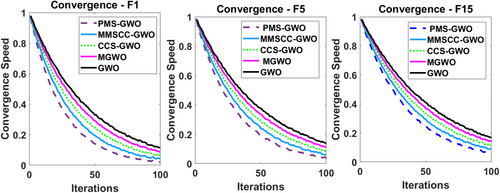
Figure 35 illustrates the impact of varying step sizes (0.001, 0.005, and 0.01) on the convergence speed of five optimization algorithms, PMS-GWO, MMSCC-GWO, CCS-GWO, MGWO, and GWO, over 100 iterations. In each of the three subplots, the x-axis represents the iteration count, while the y-axis depicts the convergence speed. Across all step sizes, PMS-GWO consistently exhibits the fastest convergence, followed by MMSCC-GWO, CCS-GWO, MGWO, and GWO, demonstrating that the relative performance of these algorithms remains consistent regardless of the step size variation, although the absolute convergence rate is slightly affected by the step size value.

Figure 36 presents trajectory plots comparing the search behavior of PMS-GWO and standard GWO algorithms in a two-dimensional space. Each subplot visualizes the path taken by the wolves during the optimization process, with the x-axis representing Dimension 1 and the y-axis representing Dimension 2. The left subplot, labeled “PMS-GWO Trajectories,” displays the search pattern for the PMS-GWO algorithm, while the right subplot, “GWO Trajectories,” shows the search pattern for the standard GWO algorithm. Both plots illustrate a dense network of lines, indicating extensive exploration and exploitation of the search space, but the visual differences suggest variations in how each algorithm navigates and converges toward potential solutions.
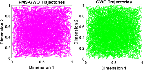
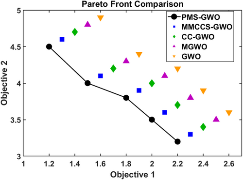
Figure 37 illustrates a comparative analysis of Pareto fronts generated for optimization algorithms: PMS-GWO, MMCCS-GWO, CC-GWO, MGWO, and GWO, within a bi-objective optimization context. PMS-GWO is represented by a continuous line connecting black circular markers, revealing a distinctive curve that indicates a unique convergence trajectory. In contrast, the remaining algorithms are depicted using discrete markers: blue squares for MMCCS-GWO, green diamonds for CC-GWO, magenta triangles for MGWO, and orange inverted triangles for GWO, facilitating a visual assessment of their respective capabilities in balancing the two objectives. The plot underscores PMS-GWO's potentially superior convergence characteristics compared to the other algorithms under evaluation.
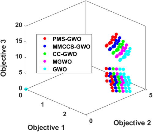
The 3D scatter plot in Figure 38 visually compares the Pareto fronts of five optimization algorithms—PMS-GWO, MMCCS-GWO, CC-GWO, MGWO, and GWO across a tri-objective optimization space. Each algorithm is represented by distinct colored markers distributed in three-dimensional space, corresponding to the values of three objectives. The plot reveals clustering patterns, suggesting the algorithms' performance in balancing these objectives. Notably, the distribution and spread of the markers indicate differences in convergence and diversity among the algorithms, thereby offering a comprehensive view of their multi-objective optimization capabilities.
5.7 Discussion on Real-World Applications
-
Energy Systems Optimization
- Problem: Energy systems, particularly those incorporating renewable sources like solar and wind, often face optimization challenges related to power generation, storage, and distribution. These systems require efficient algorithms to manage fluctuations, maximize energy output, and minimize losses.
-
PMS-GWO's Role: PMS-GWO's enhanced convergence speed and solution accuracy can be pivotal in optimizing these systems. For instance, in solar PV systems, PMS-GWO can be used to:
- ∘
Optimize the placement and sizing of solar panels to maximize energy capture.
- ∘
Develop efficient energy storage strategies to balance supply and demand.
- ∘
Improve the control of power inverters and converters for stable grid integration.
- ∘
-
Control Systems Optimization
- Problem: Control systems, used in various engineering applications, require precise tuning of parameters to achieve the desired performance. Traditional tuning methods can be time-consuming and may not yield optimal results, especially for complex systems.
-
PMS-GWO's Role: PMS-GWO's ability to quickly find accurate solutions makes it suitable for optimizing control system parameters. For example:
- ∘
Tuning PID controllers for robotic systems to achieve precise motion control.
- ∘
Optimizing the parameters of adaptive control systems for dynamic environments.
- ∘
Enhancing the performance of automated manufacturing systems by optimizing process control parameters.
- ∘
-
Mechanical Design Optimization
- Problem: Engineering design often involves optimizing mechanical components or systems for factors like weight, strength, and cost. Traditional design processes may not explore the entire design space, leading to suboptimal solutions.
-
PMS-GWO's Role: PMS-GWO can be used to optimize mechanical designs by:
- ∘
Finding optimal shapes and dimensions for structural components to minimize weight while maintaining strength.
- ∘
Optimizing the design of aerodynamic surfaces to reduce drag and improve efficiency.
- ∘
Optimizing the design of robotic arms for precise movements and efficient operation.
- ∘
Impact: PMS-GWO can result in lighter, stronger, and more efficient mechanical designs, leading to cost savings and improved performance.
Figure 39 presents a multi-faceted comparison of five algorithms (GWO, PMS-GWO, WOA, PSO, and CS) across accuracy and runtime metrics. The top-left panel displays “Algorithm Accuracy,” where PMS-GWO demonstrates superior performance with the lowest metric value, indicated by a red star. The top-right panel, “Algorithm Runtime,” reveals PMS-GWO's efficiency, showcasing the shortest execution time. The bottom-left panel, “Performance Profiles,” illustrates PMS-GWO's dominance by consistently achieving the highest probability of success across varying performance ratios. Finally, the bottom-right panel, “Accuracy vs. Runtime Trade-off,” highlights PMS-GWO's optimal balance between accuracy and runtime, positioned closest to the origin, signifying both high accuracy and low runtime. Furthermore, Table 13 depicts the various algorithms performance and statistical test results.
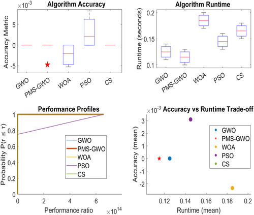
6 Conclusion
In this article, we presented the Prey-Movement Strategy Gray Wolf Optimizer (PMS-GWO), a novel extension of the traditional Gray Wolf Optimizer designed to improve the algorithm's performance in solving complex and multi-objective optimization problems. The PMS-GWO introduces several innovative strategies, including dynamic role reassignment, hybrid exploration–exploitation balance, and prey escape and mimicking behavior, which collectively enhance the algorithm's adaptability, robustness, and ability to avoid local optima. Key contributions include the dynamic reassignment of leadership roles among wolves based on cumulative fitness performance, which prevents premature convergence, and the hybrid exploration–exploitation coefficient, enabling wolves to transition smoothly between local refinement and global search. Additionally, crowding distance control and multi-phase prey movements contribute to improved diversity and more sophisticated search strategies. By introducing adaptive multi-objective prioritization and cumulative prey evaluation over multiple iterations, the algorithm effectively aligns short-term gains with long-term objectives. The performance of PMS-GWO was validated on various benchmark functions, demonstrating its superior convergence, search diversity, and solution quality compared to traditional GWO and other meta-heuristic algorithms. These enhancements make PMS-GWO a highly effective optimization tool, capable of handling complex engineering applications and diverse optimization challenges with greater precision and flexibility.
PMS-GWO improves the balance between exploration and exploitation, addressing key limitations in existing GWO variants. By optimizing prey movement strategies, it enhances convergence speed and solution accuracy while maintaining computational efficiency. However, its feasibility in industrial applications requires further validation, particularly in dynamic and large-scale problems such as energy management, logistics, and structural design. Scalability is also a crucial factor, as computational complexity must be carefully evaluated for high-dimensional problems to ensure efficiency. To extend the impact and applicability of PMS-GWO, future research should focus on its adaptation to real-world scenarios and large-scale optimization challenges. Specifically, the development of robust strategies for dynamic multi-objective optimization problems, where objectives and constraints evolve over time, is essential. This would involve incorporating mechanisms to track and respond to environmental changes, ensuring the algorithm's continued effectiveness in dynamic settings. Moreover, the integration of PMS-GWO with other evolutionary algorithms, such as differential evolution or particle swarm optimization, could lead to synergistic improvements in performance, leveraging the strengths of each algorithm. Investigating the potential of hybrid approaches, such as reinforcement learning for adaptive search or deep learning-based surrogate modeling to accelerate function evaluations, is also promising. These techniques could enable PMS-GWO to handle complex, high-dimensional problems more efficiently. Parallel computing techniques could further improve efficiency, making PMS-GWO more suitable for real-time optimization challenges. Refining these aspects would strengthen its applicability in solving complex engineering and industrial problems.
The practical applications of PMS-GWO, particularly in real-time industrial settings, are significant. For instance, in energy management, PMS-GWO can optimize the scheduling of power generation and distribution, adapting to fluctuating demand and renewable energy sources. In logistics, it can enhance route planning and resource allocation for complex supply chains, improving efficiency and reducing costs. In structural design, PMS-GWO can optimize the configuration of materials and components to enhance performance and reduce weight. These applications highlight the algorithm's potential to address complex optimization challenges in dynamic and large-scale real-world scenarios.
Additionally, future research directions could include exploring reinforcement learning for adaptive parameter tuning, combining PMS-GWO with deep learning for feature extraction and pattern recognition in complex data landscapes, or applying it to large-scale industrial optimization challenges, such as optimizing supply chains, designing complex engineering systems, or managing large-scale energy grids. These extensions would not only demonstrate the algorithm's versatility but also enhance its practical utility in addressing real-world optimization problems.
Author Contributions
Idriss Dagal: conceptualization, methodology, writing – original draft. Alpaslan Demirci: investigation, methodology, formal analysis. Ambe Harrison: software, formal analysis, methodology. Wulfran Fendzi Mbasso: writing – review and editing, project administration, supervision. Said Mirza Tercan: investigation, visualization, formal analysis. Burak Akın: investigation, visualization, project administration. Kürşat Tanriöven: data curation, project administration, visualization. Havva Aysun Sezgin Köksal: resources, project administration, supervision. Ahmet Nayir: writing – review and editing, project administration, software.
Acknowledgments
The authors have nothing to report.
Conflicts of Interest
The authors declare no conflicts of interest.
Open Research
Data Availability Statement
The data that support the findings of this study are available from the corresponding author upon reasonable request.


