Real Time Vehicle Classification Using Deep Learning—Smart Traffic Management
ABSTRACT
As global urbanization continues to expand, the challenges associated with traffic congestion and road safety have become more pronounced. Traffic accidents remain a major global concern, with road crashes resulting in approximately 1.19 million deaths annually, as reported by the WHO. In response to this critical issue, this research presents a novel deep learning-based approach to vehicle classification aimed at enhancing traffic management systems and road safety. The study introduces a real-time vehicle classification model that categorizes vehicles into seven distinct classes: Bus, Car, Truck, Van or Mini-Truck, Two-Wheeler, Three-Wheeler, and Special Vehicles. A custom dataset was created with images taken in varying traffic conditions, including different times of day and locations, ensuring accurate representation of real-world traffic scenarios. To optimize performance, the model leverages the YOLOv8 deep learning framework, known for its speed and precision in object detection. By using transfer learning with pre-trained YOLOv8 weights, the model improves accuracy and efficiency, particularly in low-resource environments. The model's performance was rigorously evaluated using key metrics such as precision, recall, and mean average precision (mAP). The model achieved a precision of 84.6%, recall of 82.2%, mAP50 of 89.7%, and mAP50–95 of 61.3%, highlighting its effectiveness in detecting and classifying multiple vehicle types in real-time. Furthermore, the research discusses the deployment of this model in low-and middle-income countries where access to high-end traffic management infrastructure is limited, making this approach highly valuable in improving traffic flow and safety. The potential integration of this system into intelligent traffic management solutions could significantly reduce accidents, improve road usage, and provide real-time traffic control. Future work includes enhancing the model's robustness in challenging weather conditions such as rain, fog, and snow, integrating additional sensor data (e.g., LiDAR and radar), and applying the system in autonomous vehicles to improve decision-making in complex traffic environments.
1 Introduction
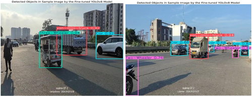
As global urbanization accelerates, the challenges associated with traffic congestion and road safety have become more pressing. Despite advances in road safety measures, traffic accidents remain a critical issue worldwide, with recent data from the World Health Organization (WHO) indicating that road traffic crashes result in approximately 1.19 million deaths annually [1]. These crashes are the leading cause of death for individuals aged 5–29 years, with vulnerable road users—such as pedestrians, cyclists, and motorcyclists—accounting for over 50% of the fatalities. The burden is disproportionately high in low- and middle-income countries, which experience 90% of global road deaths despite having fewer vehicles overall [1]. This underscores the urgent need for smarter traffic management systems and advanced vehicle detection technologies [2]. In this research, we present a novel approach to vehicle classification designed to address these road safety challenges. Our model classifies vehicles into seven distinct categories—Bus, Car, Truck, Three-wheeler, Two-wheeler, Special Vehicles, and Van or Mini-Truck—using a self-annotated custom dataset [3] with images in different traffic conditions and timings. This classification system is a critical step towards developing intelligent traffic management solutions capable of optimizing road usage and improving safety. To enhance the accuracy of the model, we leveraged the pre-trained weights of YOLOv8, a state-of-the-art deep learning model renowned for its speed and precision in object detection. By applying transfer-learning techniques, we significantly improved the performance of the model, enabling more accurate vehicle classification even with limited dataset sizes. The detection and classification of the vehicles can be seen in Figure 1.
1.1 Highlights
- The model is trained using a custom dataset, with all images manually annotated to enhance real-time performance and ensure accurate vehicle classification [4].
- Pre-trained YOLOv8 weights were used to boost model accuracy, leveraging transfer learning [5, 6] for faster convergence and improved precision in detecting seven distinct vehicle types.
- The model demonstrates strong potential for integration into smart traffic management systems, contributing to better traffic flow and enhanced road safety.
2 Literature Review
A literature survey was conducted to review the existing works in the field. The following summary presents the key findings from chapters related to the proposed research.
Lv et al. proposed an ensemble approach combining two state-of-the-art deep learning models, EfficientDet and YOLOv8, to address challenges associated with diverse vehicle characteristics and varying lighting conditions. The study utilized both RGB and thermal images from the FLIR dataset to enhance detection accuracy, particularly in low-light scenarios where traditional methods struggle. By incorporating extensive data augmentation techniques to address class imbalances, the ensemble model was trained to generalize effectively across different vehicle types and environments. The experimental results demonstrated that the ensemble method significantly outperformed the individual models, achieving a mean average precision (mAP) of 95.5% on thermal images and 93.1% on RGB images, with an average recall (AR) of 0.93 for thermal images. The integration of EfficientDet's BiFPN for multi-scale detection and YOLOv8's speed and real-time accuracy resulted in a robust detection system. The use of majority voting to combine model predictions further enhanced the classification performance. This study h ighlights the potential of ensemble learning techniques to overcome the limitations of individual deep learning models, making the system suitable for real-world applications, particularly in intelligent traffic management systems [7].
Marathe et al. introduced WEDGE, a multi-weather autonomous driving dataset generated using vision-language models such as DALL-E. The dataset contains 3360 images across 16 extreme weather conditions, manually annotated with over 16,500 bounding boxes for tasks like weather classification and 2D object detection. The motivation behind WEDGE is to enhance the robustness of autonomous vehicle perception systems, particularly in adverse weather conditions, which are often underrepresented in traditional datasets. The dataset showed its utility in improving state-of-the-art (SOTA) performance in real-world weather benchmarks such as DAWN, with significant improvements in detecting classes like trucks. By fine-tuning object detectors on WEDGE, the researchers achieved an increase in average precision by 4.48 points for trucks. The study emphasizes the potential of synthetic datasets to bridge gaps in sim2real transfer, improving detection in underrepresented weather conditions for autonomous driving tasks [8].
Dong et al. present an enhanced approach to vehicle classification, leveraging advancements in deep learning and vision transformers. Traditional methods, particularly convolutional neural networks (CNNs), were effective at capturing local features but struggled with global feature representation. The paper proposes a novel model, IND-ViT, which integrates CNNs to address local feature loss in vision transformers. This hybrid architecture, combining a CNN-In D module and a sparse attention module, improves the model's ability to detect subtle distinctions between similar vehicles and enhances overall feature extraction. Through the use of a contrast loss function, the model increases intra-class consistency and inter-class distinction. Experimental results show that IND-ViT outperforms traditional ViT and CNN-based models on datasets like BIT-Vehicles, CIFAR-10, and Oxford Flower-102, with improvements in classification accuracy of up to 7.54% for certain datasets. The method strikes a balance between accuracy and real-time performance, showcasing its potential for applications in autonomous driving systems [9].
Trivedi et al. present an advanced approach to vehicle classification using computer vision techniques. The study highlights the significance of vehicle classification in smart transportation systems, emphasizing its role in traffic management and automated toll collection. The authors utilize Speeded-Up Robust Features (SURF) for feature extraction and employ multiple classifiers, including Support Vector Machines (SVM), Decision Trees, and K-Nearest Neighbors (KNN), to categorize vehicles into three classes: bikes, cars, and trucks. Their methodology is validated on a dataset of approximately 11,000 images, achieving a high classification accuracy of 91% using a Medium Gaussian SVM classifier. The research underscores the challenges posed by varying lighting conditions, image resolutions, and real-time constraints, offering insights into feature extraction techniques and classifier performance. Additionally, the paper discusses the limitations of traditional classification approaches and suggests potential improvements using deep learning-based architectures for enhanced accuracy and real-time application in Intelligent Transportation Systems (ITS) [10].
Wang et al. present a deep learning-based approach to vehicle classification for intelligent transportation systems. The study leverages Faster R-CNN for vehicle detection and classification, outperforming traditional machine learning techniques. The proposed system effectively classifies vehicles into cars, trucks, minivans, and buses with a mean average precision (mAP) of 81.05% and achieves over 90% accuracy for cars and trucks. The model is trained on a dataset of over 60,000 labeled images and optimized for real-time performance, operating at 0.354 s per image on an NVIDIA Jetson TK1 embedded system. The authors highlight challenges such as varying illumination, image scales, and angles, demonstrating that convolutional neural networks (CNNs) provide robust feature extraction and classification capabilities. The research concludes that deep learning significantly enhances vehicle classification accuracy and efficiency, paving the way for real-time intelligent traffic monitoring and autonomous driving applications [11].
Osman et al. present a deep learning-based approach to real-time vehicle detection and classification in traffic surveillance systems. The study utilizes the YOLOv8 (You Only Look Once) object detection algorithm, a convolutional neural network (CNN)-based model, to classify vehicles into seven categories: car, bike, SUV, van, bus, truck, and person. The authors trained the model on real traffic video data collected from 10 intersections, using bounding box annotations for precise vehicle detection. The proposed method achieves a classification accuracy of 91%, outperforming traditional fixed-duration traffic signalization systems by dynamically adjusting green light durations based on real-time vehicle density and class distribution. The study highlights improvements in reducing traffic congestion, fuel consumption, air pollution, and driver stress through adaptive traffic signal control. The results demonstrate that deep learning techniques, particularly YOLOv8, significantly enhance vehicle recognition and smart traffic management systems, making them more efficient and responsive to real-world conditions [12].
3 Vehicle Classification System
Our vehicle detection and classification model is based on YOLOv8, a state-of-the-art object detection framework known for its real-time processing capabilities and accuracy. We have designed the model to identify vehicles across seven key classes that contribute differently to traffic congestion:
3.1 Bus
Buses are a major contributor to road congestion, particularly when they occupy central lanes. Due to their large size, buses require more space and time to move through traffic, often leading to a slower traffic flow behind them.
3.2 Two-Wheeler
This class includes motorcycles, bicycles, and scooters. While two-wheelers are widely used, especially in urban environments, they have a relatively minimal impact on traffic congestion due to their small size and ability to navigate through crowded spaces. However, they do contribute to congestion at intersections and in side lanes.
3.3 Car
Cars are the most common form of personal transportation and can vary significantly in terms of their impact on traffic. When present in large numbers, cars can contribute to traffic bottlenecks, especially in narrow or congested roadways.
3.4 Truck
This class includes large trucks, containers, and other heavy-duty vehicles. Trucks, due to their size and slower acceleration, are a major factors in creating traffic jams, particularly when they occupy multiple lanes or travel through urban areas during peak hours.
3.5 Van or Mini-Truck
Smaller utility vehicles such as vans, ambulances, and mini-trucks fall into this category. While they are smaller than full-sized trucks, they still occupy more space than personal vehicles and can contribute to congestion, particularly during high-traffic periods or emergencies.
3.6 Three-Wheeler
Vehicles such as autorickshaws and e-rickshaws, commonly used for short-distance public transport, often contribute to roadside congestion. These vehicles tend to cluster near intersections or sidewalks, which can disrupt the flow of traffic in adjacent lanes.
3.7 Special Vehicles
This class includes vehicles used for specific purposes such as construction equipment (e.g., JCBs, cement mixers) or emergency response vehicles. Though not frequently present on the roads, they can cause significant disruptions when they are in use, especially in areas not designed to accommodate them.
4 Self-Created Dataset
The dataset [3] for real-time vehicle classification was carefully curated and structured into train (800 images), test (215 images), and validation (311 images) sets, ensuring a balanced evaluation of the model's performance as shown in Table 1. To enhance data quality and consistency, auto-orientation of pixel data was applied by stripping EXIF metadata, and all images were resized to 640 × 640 pixels using a stretching transformation. To improve model robustness and generalization, extensive data augmentation was performed as mentioned in Table 2, generating three augmented versions of each image (800 × 3 = 2400 images for train set). Augmentations included a 50% probability of horizontal flipping, random rotation between −15° and +15°, random shear transformations between −10° and +10° both horizontally and vertically, random exposure adjustments within a −10% to +10% range, and the introduction of salt and pepper noise to 0.1% of pixels to simulate real-world variations and environmental noise. These preprocessing and augmentation strategies contribute to a diverse and resilient dataset, enhancing the model's ability to handle different lighting conditions, orientations, occlusions, and image distortions, ultimately improving its robustness in real-time traffic applications.
| Split | Before argumentation (Raw dataset) | After argumentation |
|---|---|---|
| Train | 800 | 2400 |
| Test | 215 | 215 |
| Validate | 311 | 311 |
| Total | 1326 | 2926 |
| Method | Settings |
|---|---|
| Flip | Horizontal |
| Rotation | Between −15° and +15° |
| Shear (Horizontal and Vertical) | Between −10° and +10° |
| Exposure | Between −10 and +10% |
| Noise | Up to 10% of pixels |
5 Used Methodology
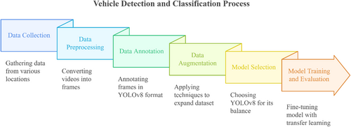
In many low- and middle-income countries, despite advancements in hardware such as better cameras and sensors, traffic management continues to face challenges due to limited resources. This research addresses these challenges by leveraging advanced convolutional neural network (CNN) models, specifically YOLOv8, to classify vehicles into seven distinct categories. To optimize the model for real-time performance in low-resource environments, transfer learning [13] was employed, utilizing pre-trained weights from YOLOv8. This paper details the entire workflow, from dataset creation to model training and evaluation, highlighting the potential of the model for integration into smart traffic systems aimed at reducing accidents and improving traffic flow, as demonstrated in Figure 2.
5.1 Data Collection
Data was collected from three different locations, each with varying traffic conditions and vehicle densities. A total of seven videos were recorded from different angles to capture a diverse range of vehicle types and traffic environments. The use of mobile cameras ensured adequate image quality while maintaining accessibility in resource-limited environments. This multi-angle approach provided a comprehensive dataset reflecting real-world traffic scenarios.
5.2 Data Preprocessing
Once collected, the videos were converted into individual frames, preparing the data for training. This process allowed us to extract relevant instances of traffic patterns, ensuring that each frame captured the unique dynamics of traffic flow and vehicle types across different locations.
5.3 Data Annotation
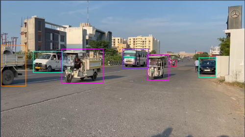
Each frame was manually annotated in the YOLOv8 format, as shown in Figure 3. The classification system was based on seven distinct vehicle categories: bus, two-wheeler, car, truck, van or mini-truck, three-wheeler, and special vehicles. These categories were designed to encompass nearly all common road vehicle types. The meticulous annotation process ensured high-quality, labeled data, providing the model with the necessary accuracy for real-time vehicle detection and classification.
The annotation count of the different classes of vehicles is given in Table 3.
| Class | Annotation count |
|---|---|
| Car | 2002 |
| Two-wheeler | 996 |
| Bus | 484 |
| Van or mini-truck | 409 |
| Three-wheeler | 290 |
| Truck | 219 |
| Special vehicle | 161 |
| Total | 4561 |
5.4 Data Augmentation
To enhance the model's ability to generalize across varying traffic conditions, data augmentation techniques were applied. These techniques included random rotation, horizontal flipping, shear adjustments, exposure variations, and the introduction of noise. This augmentation expanded the dataset [3] from 1326 images to 2926 images (85%–90% custom images [3], 10%–15% from free sources [14, 15]). The added variability allowed the model to handle diverse real-time traffic conditions effectively.
5.5 Model Selection
YOLOv8 was selected due to its strong balance between speed and accuracy, making it well- suited for real-time traffic management applications [16]. The model's architecture, including anchor-free bounding box prediction, reduces computational complexity and adapts better to objects with varying aspect ratios, a key requirement for vehicle detection. We compared multiple algorithms based on their features and architecture, which you can see in Table 4.
| Algorithm | Speed (FPS) | mAP (COCO) | Architecture | Key improvements |
|---|---|---|---|---|
| YOLOv8 | 65 (Tesla V100) | 50.5% | CNN + CSPNet | Improved feature fusion, better anchor-free detection, more efficient training |
| YOLOv5 | 140 (Tesla V100) | 50.3% | CSPDarknet | Optimized for fast inference, better data augmentation tools |
| EfficientDet | 25–30 (TPU) | 52.2% | BiFPN + EfficientNet | Efficient feature fusion and scaling, lightweight models |
| Faster R-CNN | 10–15 (V100) | 42.0% | R-CNN with region proposal networks | Strong accuracy, but slower inference speed |
| YOLOv4 | 62 (Tesla V100) | 43.5% | CSPDarknet + PAN | Improved speed and accuracy using PANet and CSP connections |
| SSD | 45 (V100) | 41.2% | Multi-scale feature maps | Balances speed and accuracy, but lower mAP compared to YOLO family |
| RetinaNet | 25–30 (V100) | 39.1% | ResNet + FPN | Introduced focal loss to handle class imbalance |
5.6 Model Fine-Tuning and Evaluation
We utilized transfer learning [13] by fine-tuning the pre-trained weights of YOLOv8 to suit the specific characteristics of our dataset. The model's ability to handle multiple vehicle classes in a single image improved its accuracy and ensured it could generalize across real-world traffic scenarios. Standard evaluation metrics were used to assess the model's performance and ensure it met the requirements for integration into smart traffic management systems. Finally, the model was fine-tuned to adapt to the unique traffic conditions observed in the dataset. This step ensured the model's effectiveness in detecting and classifying vehicles in real time, thereby making it suitable for live traffic monitoring and control systems aimed at improving traffic flow and reducing congestion.
6 Model Implementation and Fine-Tuning
This section discusses the specifics of the YOLOv8 model, its architecture, the fine-tuning process, and detailed augmentation techniques applied during training.
6.1 YOLOv8
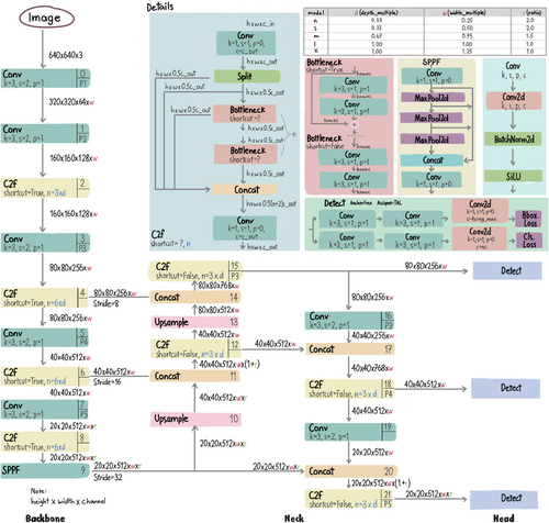
YOLOv8 builds upon the advancements of its predecessors in the YOLO family [17], incorporating state-of-the-art developments in neural network architecture and training strategies. Like earlier versions, YOLOv8 integrates object localization and classification within a unified, end-to-end differentiable framework, effectively balancing speed and accuracy. The model's architecture is structured around three critical components, as shown in Figure 4.
6.1.1 Backbone
YOLOv8 utilizes an advanced convolutional neural network (CNN) backbone designed to capture multi-scale features from input images [18, 19]. This backbone, potentially an enhanced version of CSPDarknet or another efficient architecture, extracts hierarchical feature maps that encompass both low-level textures and high-level semantic information. These feature maps are vital for accurate object detection. Optimized for computational efficiency and accuracy, the backbone incorporates depthwise separable convolutions or similar efficient layers, reducing computational costs while preserving high representational power.
6.1.2 Neck
The neck module is responsible for refining and fusing the multi-scale features obtained from the backbone. It builds on an optimized Path Aggregation Network (PANet) [19], designed to enhance information flow across multiple feature levels. This multi-scale integration is crucial for detecting objects of various sizes, and YOLOv8 likely incorporates improvements to the original PANet to reduce memory consumption and increase computational efficiency.
6.1.3 Head
The head module generates the final predictions—bounding box coordinates, object confidence scores, and class labels—from the processed features. One notable innovation in YOLOv8 is the shift to an anchor-free approach [20] for bounding box prediction, moving away from the anchor-based methods employed in earlier versions. This anchor-free design simplifies the prediction process, reduces hyperparameter dependency, and enhances adaptability to objects with varying aspect ratios and scales [20]. By synthesizing these architectural improvements, YOLOv8 demonstrates superior performance in object detection tasks, offering advancements in accuracy, speed, and model flexibility [21]. These enhancements mark a significant step forward in object detection methodologies, enabling more efficient and precise models for practical applications.
6.1.4 Improvements in YOLOv8
- Anchor-Free Detection: YOLOv8 moves toward anchor-free detection, reducing the complexity of hyperparameters related to anchor boxes. This allows for simpler and faster training and inference.
- Network Efficiency: YOLOv8 incorporates advancements in network design, such as better feature fusion and optimized architecture, to improve both speed and accuracy.
- Model Flexibility: YOLOv8 is designed to be versatile, supporting tasks beyond object detection, such as instance segmentation and keypoint detection.
- Better Data Augmentation: The model leverages modern augmentation techniques, improving robustness against overfitting and enhancing performance on diverse datasets [18].
- Loss Function Enhancements: YOLOv8 utilizes newer loss functions and optimizations that enhance object localization and classification accuracy, particularly for smaller objects.
6.2 Data Preprocessing and Augmentation
The dataset used for training the YOLOv8 model consists of 2926 images, all annotated in YOLOv8 format. Each vehicle was labeled based on the seven distinct classes described earlier, and the data was prepared using a series of pre-processing and augmentation techniques to enhance the model's ability to generalize in real-time applications.
6.2.1 Data Preprocessing
- Auto-orientation of pixel data: Images were automatically corrected for orientation, with EXIF-orientation metadata stripped to standardize the image direction.
- Resizing to 640 × 640 (stretch): All images were resized to a resolution of 640 × 640 pixels to match the input requirements of the YOLOv8 model. This uniform size allows for consistent image dimensions, ensuring optimal performance during training and inference.
6.2.2 Data Augmentation
- Horizontal flip (50% probability): Images were randomly flipped horizontally with a 50% probability, which simulates real-world variations and improves the model's ability to detect vehicles in different orientations.
- Random rotation (−15° to +15°): Each image was randomly rotated by an angle between −15° and +15° to account for diverse camera angles and perspectives in real-world scenarios.
- Random shear (±10° horizontally and vertically): A shear transformation was applied to each image with a random degree between −10° and +10° both horizontally and vertically. This helps in simulating distortions that may occur during data capture.
- Exposure adjustment (−10% to +10%): The exposure of the images was randomly adjusted by ±10% to simulate variations in lighting conditions, further enhancing the model's ability to adapt to different real-world environments.
- Salt and pepper noise (0.1% of pixels): To simulate potential noise in images (e.g., from poor-quality cameras), salt and pepper noise was applied to 0.1% of the image pixels. This encourages the model to become more resilient to image noise and imperfections.
A notable innovation in YOLOv8 is its shift from the traditional anchor-based bounding box prediction to an anchor-free approach [22]. This methodology reduces computational complexity by eliminating the need for predefined anchor boxes, enhancing model efficiency. It also improves the model's adaptability in detecting objects of varying aspect ratios and scales, offering increased flexibility across a wide range of object detection tasks. This comprehensive augmentation process, combined with the anchor-free bounding box prediction, was instrumental in expanding the dataset size and improving the model's performance across diverse traffic conditions. This ensures that the model generalizes well for real-time vehicle detection and classification tasks.
6.3 Fine-Tuning the Model
- Custom Dataset: The model was trained on our annotated dataset using a dataset configuration file that defined the class labels and dataset structure.
- Training Configuration: We trained the model for 100 epochs, with each input image resized to 640 × 640 pixels for consistency. The batch size was set to 90 images per iteration, allowing efficient GPU utilization (device = 0 for CUDA).
- Optimization Strategy: The training used an adaptive optimizer (optimizer = ‘auto’), which selects the best optimizer automatically from a list of options (e.g., SGD, Adam, and RMSProp). The initial learning rate was set to 0.0001, gradually decreasing to 0.1 of the initial value (via lrf).
- Early Stopping: To prevent overfitting, we implemented an early stopping mechanism with a patience of 50 epochs, meaning the training would stop if no improvement were observed for 50 consecutive epochs.
- Regularization: Dropout with a rate of 0.1 was applied to prevent overfitting, helping the model to generalize better on unseen data.
- Reproducibility: A fixed random seed (seed = 0) ensured the results were reproducible.
This fine-tuning process allowed the model to adapt efficiently to our specific vehicle classification task, ensuring high performance in real-time detection and classification [4].
6.4 Loss Calculation
YOLOv8's loss function is meticulously designed, comprising three key components to optimize performance across object classification, localization, and Objectness prediction.
6.4.1 Focal Loss for Classification
- pt is the model's estimated probability for the correct class. Specifically, for binary classification:
- if the true label is 1
- if the true label is 0
- αt is a weighting factor for balancing the importance of positive versus negative classes (optional).
- γ is the focusing parameter that adjusts the rate at which easy examples are down-weighted. Typically, γ is set to 2. As γ increases, the loss function focuses more on hard-to-classify examples.
- log() is the logarithmic term from the standard cross-entropy loss.
6.4.2 IoU Loss for Localization
To refine the model's ability to localize objects, YOLOv8 employs Intersection over Union (IoU) loss. This component of the loss function enhances the accuracy of bounding box predictions by penalizing inaccurate localizations, thereby improving the model's precision in object detection tasks.
6.4.3 Objectness Loss
- N is the number of predicted bounding boxes.
- is the predicted objectness score for the ith bounding box.
- is the ground truth objectness label for the ith bounding box (1 if the box contains an object, 0 otherwise).
-
BCE refers to Binary Cross-Entropy loss, which is given by:
7 Results and Performance Metrics
This section provides a comprehensive evaluation of the vehicle classification model's performance, including key metrics such as precision, recall, and mean average precision (mAP) across different vehicle classes. This section highlights the model's robustness, demonstrating its ability to accurately detect and classify vehicles in real-time scenarios. The performance of each class—Bus, Car, Truck, Van or Mini-Truck, Two-Wheeler, Three-Wheeler, and Special Vehicles, and model performance is visualized through loss curves and precision-recall metrics. Table 5 shows the performance metrics of the model across various classes of vehicles. The model took 1.696 h for 100 epochs to run.
| Class | Precision | Recall | mAP50 | mAP50–95 |
|---|---|---|---|---|
| All | 84.6 | 82.2 | 89.7 | 61.3 |
| Bus | 82.2 | 87.8 | 93.0 | 69.6 |
| Car | 81.9 | 91.0 | 92.9 | 65.7 |
| Special Vehicles | 78.0 | 87.2 | 88.7 | 52.8 |
| Three-Wheeler | 98.3 | 79.3 | 89.2 | 62.0 |
| Truck | 83.2 | 73.3 | 87.9 | 66.9 |
| Two-Wheeler | 82.8 | 76.8 | 86.9 | 48.7 |
| Van or Mini-Truck | 85.5 | 80.2 | 89.3 | 63.7 |
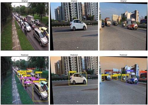
Few of the model's predictions are shown in the Figure 5, showcasing its effectiveness in real-world applications.
7.1 Precision
The model achieved a precision of 0.846 (or 84.6%), meaning that out of all vehicle detections made by the model, 84.6% were correctly classified.
7.2 Recall
The model recorded a recall of 0.822 (or 82.2%), indicating that it successfully detected 82.2% of all vehicles present in the images.
7.3 Mean Average Precision (mAP)
7.3.1 mAP50
7.3.2 mAP50–95
7.4 Fitness
The fitness score is a composite metric that combines various performance indicators, such as precision, recall, and mAP, to provide a comprehensive assessment of a model's overall effectiveness. It helps to balance the trade-offs between different performance measures to evaluate the model's general capability. The fitness score can be calculated using a weighted formula that incorporates the individual metrics, though the exact formula may vary based on the specific weighting applied. The model achieved a fitness score of 0.642 (or 64.2%), reflecting a balanced performance across precision, recall, and detection accuracy.
7.5 PR Curve
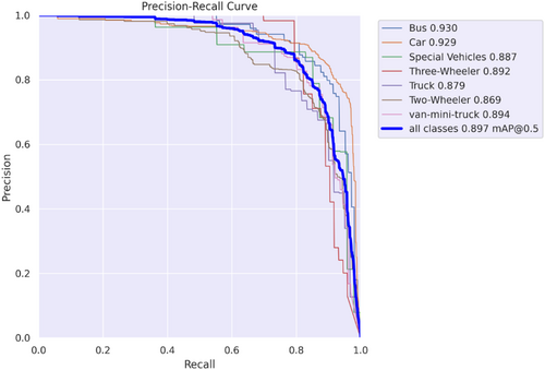
The PR (Precision-Recall) curve illustrates the trade-off between precision and recall for the classification model [24]. Precision measures the accuracy of positive predictions, while recall indicates the proportion of actual positives correctly identified. The curve is especially useful for imbalanced datasets. High precision with low recall means the model is conservative, making fewer but more accurate positive predictions, while high recall with low precision indicates more positive instances are identified but with more false positives. The area under the PR curve (AUC-PR) reflects overall model performance, with a larger area indicating a better ability to distinguish between classes. The PR curve for the developed model can be seen in Figure 6.
7.6 Confusion Matrix
- True Positives (TP): Instances correctly predicted as the positive class.
- True Negatives (TN): Instances correctly predicted as the negative class.
- False Positives (FP): Instances incorrectly predicted as positive, also known as Type I errors.
- False Negatives (FN): Instances incorrectly predicted as negative, also known as Type II errors.
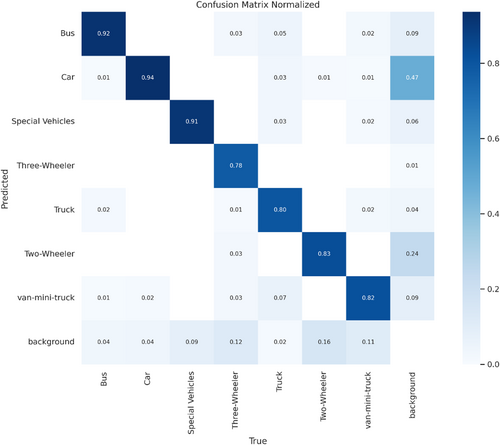
By examining these values, the confusion matrix provides insights into different metrics, such as accuracy, precision, recall, and F1 score. It allows for a detailed breakdown of the model's performance, showing not only how many predictions are correct but also where the model makes mistakes, whether it confuses certain classes, and how balanced the predictions are across categories. This is particularly useful when dealing with imbalanced datasets, where a high overall accuracy might be misleading. You can see the confusion matrix for the model in Figure 7.
7.7 F1-Confidence Curve
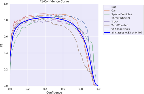
The F1-Confidence Curve is a graphical representation that depicts the relationship between the F1 score and various confidence thresholds for a multi-class vehicle detection model. The F1 score, which balances precision and recall, is particularly useful in assessing model performance across different vehicle categories. As the confidence threshold varies, the F1 score fluctuates, reflecting the model's effectiveness in accurately detecting and classifying vehicles. A higher F1 score indicates a better balance between precision (true positive predictions) and recall (actual positive instances), essential for effective vehicle classification. In the graph as shown in Figure 8, the blue curve shows the average F1 score across all classes, peaking at 0.83 when the confidence score is 0.407. This optimal threshold enhances the model's practical utility in real-time vehicle detection systems, providing insights into the best confidence levels for deployment.
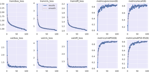
Now in Figure 9 there are some other metrics and graphs for the better understanding of the overall model and its losses.
7.8 Loss Curves Analysis
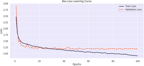
7.8.1 Box Loss Learning Curve
It tracks the model's ability to accurately predict bounding boxes for detected vehicles, as shown in Figure 10. Both the training and validation losses start high, rapidly decreasing as the model learns, and eventually stabilize around 1.00 after 100 epochs. This shows that the model has learned to predict bounding boxes effectively, with a consistent performance between training and validation sets, indicating minimal overfitting.
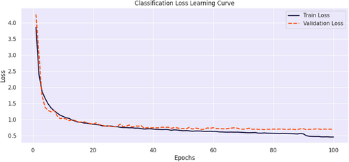
7.8.2 Classification Loss Learning Curve
It shows the model's performance in classifying vehicle types as shown in Figure 11. The loss decreases sharply in the initial epochs, with both training and validation losses converging towards 1.00. This indicates that the model is able to distinguish between different vehicle classes effectively, and the closeness of the training and validation curves suggests good generalization across the dataset.
7.8.3 Distribution Focal Loss Learning Curve
It addresses class imbalance, helping the model focus on harder-to-classify instances as shown in Figure 12. The training loss stabilizes near 1.00, while the validation loss remains slightly higher, suggesting that the model effectively handles imbalanced vehicle classes without major overfitting, although there may be room for improvement in dealing with certain complex cases.
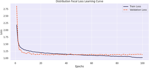
In all three graphs, the training and validation losses remain closely aligned, highlighting the model's robustness and efficiency in predicting bounding boxes and classifying vehicles while avoiding overfitting.
8 Conclusion and Discussion
This research introduces a real-time vehicle classification model utilizing the YOLOv8 framework, built on a self-annotated custom dataset comprising seven vehicle categories: Bus, Car, Truck, Van or Mini-Truck, Two-Wheeler, Three-Wheeler, and Special Vehicles. The model effectively addresses the complexities of traffic management in resource-constrained environments, achieving high precision and recall through transfer learning and efficient computational performance. The comprehensive workflow of data collection, annotation, preprocessing, and augmentation highlights the rigorous methodology that underpins the model's robustness. Its successful integration into intelligent traffic management systems offers improved traffic flow and enhanced road safety, especially in low- and middle-income countries with limited infrastructure.
9 Limitations and Future Scopes
Despite achieving high classification accuracy, the proposed real-time vehicle classification system has certain limitations. First, the dataset, although diverse, may not fully represent extreme environmental conditions such as heavy fog, nighttime glare, or severe weather, which could impact model performance. Second, the resizing of images to 640 × 640 pixels using a stretch transformation may introduce distortions, potentially affecting object shape integrity. Additionally, while YOLOv8 performs well in real-time detection, its computational requirements may pose challenges for low-power embedded devices, limiting its deployment in resource-constrained environments. The salt and pepper noise applied to only 0.1% of pixels may not fully simulate real-world noise levels caused by motion blur, occlusions, or sensor defects. Moreover, the augmentation strategy does not include adversarial perturbations, which could make the model vulnerable to minor adversarial changes. Future work can address these limitations by incorporating domain adaptation techniques, higher-resolution datasets, and optimizing inference for edge devices.
Author Contributions
Tejasva Maurya: conceptualization, methodology, investigation, writing – original draft, writing – review and editing. Saurabh Kumar: conceptualization, methodology, visualization, validation, writing – original draft, writing – review and editing. Mritunjay Rai: conceptualization, validation, writing – original draft, writing – review and editing. Abhishek Kumar Saxena: conceptualization, methodology, investigation, validation, project administration, resources, writing – original draft, writing – review and editing. Neha Goel: conceptualization, validation, project administration, supervision, writing – original draft, writing – review and editing. Gunjan Gupta: conceptualization, writing – original draft, supervision, project administration, resources, validation, methodology.
Conflicts of Interest
The authors declare no conflicts of interest.
Open Research
Data Availability Statement
The data that support the findings of this study are available from the corresponding author upon reasonable request.


