Volume 7, Issue 3 e70065
RESEARCH ARTICLE
Open Access

Impact of Temperature Variability on the Caputo Fractional Malaria Model

Dawit Kechine Menbiko

Corresponding Author

Dawit Kechine Menbiko

College of Natural Sciences, Jimma University, Jimma, Oromia, Ethiopia

Correspondence: Dawit Kechine Menbiko ([email protected])

Contribution: ​Investigation, Writing - original draft, Methodology, Software, Formal analysis

Search for more papers by this author
Chernet Tuge Deressa

Chernet Tuge Deressa

College of Natural Sciences, Jimma University, Jimma, Oromia, Ethiopia

Contribution: Supervision, Resources, Conceptualization

Search for more papers by this author
First published: 23 March 2025

ABSTRACT

Malaria is one of the most common illnesses in the world. This paper aims to analyze the age-related characteristics of malaria in human hosts by exploring Caputo fractional-order models with temperature variability. The model is well-posed both mathematically and epidemiologically. According to the model, the likelihood of disease transmission and the rate of mosquito contact are important determinants of the disease's spread. The model's stability and steady states are investigated. To determine the fundamental reproduction number, the next-generation method is used. The endemic equilibrium is shown to be locally and globally asymptotically stable under the conditions for the stability of the equilibrium points, whenever the basic reproduction number is bigger than unity. The study examined the combined effects of fractional order and temperature variability on malaria dynamics. Nevertheless, we demonstrated that the endemic equilibrium point is unique. MATLAB was used to simulate Caputo fractional order with and without temperature variability and to apply the Adams–Bashforth–Moulton numerical approach. The model suggests that, in addition to any other strategy that lowers the incidence of malaria infection, efforts should be made to decrease mosquito populations and contact rates using chemical or biological therapies.

1 Introduction

The malaria parasite, which infects people, has been carried by mosquitoes for millions of years. It is endemic in over 85 countries [1]. According to the World Health Organization (WHO), about half of the world's population is at risk of contracting malaria. In 2018, an estimated 405,000 people died, and 228 million cases of malaria were reported globally, with 93% of cases and 94% of fatalities occurring in Africa [2]. Africa accounts for a disproportionately high percentage of malaria cases worldwide. Furthermore, in 2021, malaria accounted for 95% of cases and 96% of deaths. More than 80% of malaria deaths in the WHO African area occurred among children under the age of 5. In addition to being more badly impacted by the disease than older children, children under 5 make up two-thirds of all recorded deaths [3]. Over 60% of Ethiopia's population lives in areas where malaria is likely to spread, and 68% of the country is conducive to malaria transmission [3]. Rainfall and temperature are the two primary determinants of malaria [4, 5]. The impact of pesticide resistance on the mosquito population needs to be assessed because indoor residual spraying (IRS) and insecticide-treated bed nets (ITNs) are frequently used to prevent malaria [6-8].

To gain insights into the kinetics of transmission and identify relevant preventive measures, a mathematical model should be developed. According to Ross [9], malaria can be abolished if the mosquito population is brought down to below a particular threshold. Many models were developed by different researchers using a range of parameters in accordance with the Ross model. For Example, Macdonald [10] modified Ross's model and came to the conclusion that, in regions where malaria transmission is severe, reducing mosquito populations alone will neither eliminate or lessen the disease's impact. Numerous researchers have created mathematical models to assess the impact of climate change and seasonality on the dynamics of malaria transmission, as demonstrated in [11-13]. Researchers in [14] examine an age-structured mathematical model for the kinetics of malaria spread with an asymptomatic carrier and temperature fluctuations. Researchers in [15] proposed and analyzed a nonlinear deterministic mathematical model of malaria transmission dynamics by incorporating awareness of people as one of the controlling strategies. Additionally, Keno et al. [16] presented a nonlinear deterministic mathematical model for malaria transmission dynamics incorporating climatic variability as a factor. The influence of temperature and rainfall abundance on malaria transmission dynamics was explored, and an integer-order mathematical model that integrates such climatic parameters into the dynamics of the human host-mosquito vector system was constructed by [17]. Using epidemiological information gathered from the western region of Ethiopia, the researchers in [18] investigated how variations in climate impact the spread of malaria.

Several scholars apply fractional derivatives in different areas of study. For instance, the fractional difference model is used by the researchers to generate and analyze computer virus spread by utilizing the Atangana–Baleanu sense [19]. A new fractional model of the human liver is created with an exponential kernel and the Caputo–Fabrizio derivative [20]. The pantograph differential equation is reformed and evaluated in the Riemann–Liouville and Caputo frameworks using newly specified conformable operators [21, 22]. Science et al. [22] presents a mathematical model for the Caputo fractional-order derivative's role in COVID-19 transmission. The qualitative theory of the solutions of a multi-point sequential Caputo-type p-Laplacian coupled system, including the generalized Hyers–Ulam stability and Hyers–Ulam stability is examined in [23]. A fractional generalized Sturm–Liouville–Langevin (FGSLL) equation using the Ψ-Caputo fractional derivative was considered by the researchers using a modified argument in [24]. The fractional-order diabetic awareness model is solved using the efficient homotopy analysis method (HAM) [25, 26]. Rai et al. [26] examine how environmental contamination affects the coronavirus pandemic's propagation. With fractional-order derivatives, the impact of population migration and the backward bifurcation phenomena on the TB epidemic's prevalence is demonstrated in [27]. In [28], a nonlinear vector–host model is used to study the dynamics of dengue virus transmission. Mondal and Khajanchi [29] outline the nonlinear mathematical model of how media awareness can be used to apply optimal control to slow the spread of infectious diseases.

In [30], integer and fractional-order models are used to analyze the dynamics of malaria in a human host with varying age structures. The mathematical model of transmission co-infection of TB in the HIV community with a non-singular kernel and fragmental-fractional modeling in the mathematical epidemiology of TB disorders is investigated by researchers in [31, 32]. The non-singular Mittage–Leffler derivative, which incorporates co-infection of HBV and HCV, is described by the fractional mathematical model [33]. In [34], the Caputo fractional derivatives are used to analyze the four-dimensional hyperchaotic Lorenz–Steno technique. The models developed with classical differential equations are subject to a number of limitations. In fact, without memory or non-local effects, the crossover behavior of physical or biological processes cannot be described [30]. Fractional differential operators based on a power-law kernel were first introduced by Riemann–Liouville and Caputo. However, the unique kernels of these operators limit their applicability to the simulation of biological and other physical processes [35, 36].

The Caputo fractional derivative has the benefit of enabling the application of beginning and boundary conditions in real-world scenarios. It is the best fractional operator to utilize when simulating real-world issues [37]. Parham and Michael developed an integer-order mathematical model that specified the adult mosquito birth rate as a function of temperature and rainfall to investigate the effects of environmental factors on the dynamics of transmission [11]. An age-structured deterministic malaria transmission dynamics model is analyzed in [38]. A temperature-dependent classical order model was created by Agusto et al. [13] to assess the role of temperature variation on malaria transmission dynamics. Flashade and Agusto [39] examined the most effective malaria prevention strategies in the face of temperature change in 2020, using a temperature-dependent classical order malaria model. The Mathematical model that tracks the dynamics of malaria in the human host and mosquito vector with temporary immunity is analyzed in [40].

To the best of our understanding, numerous researchers conducted climate variability-dependent classical order malaria models, and some conducted fractional-order derivatives for malaria transmission dynamics; almost none of the studies incorporate the Combined impact of both temperature variability and Caputo fractional order of age-structured malaria models on the malaria transmission dynamics, including a protected compartment with individuals who use intervention mechanisms to control the spread of malaria transmission. The purpose of our age-structured mathematical malaria model is to incorporate Caputo fractional-order derivatives with the impact of temperature variations and a protected compartment with individuals who use intervention mechanisms to control the spread of malaria transmission.

Structure of the study incorporates: Section 2 covers the mathematical preliminary, Section 3 develops the mathematical model formulation, Section 4 analyzes the fractional model, Section 5 discusses equilibrium points and stability analysis, Section 6 examines model analysis with temperature-dependent parameters, Section 7 presents the numerical scheme and simulation, Section 8 provides results, and Section 9 concludes.

2 Mathematical Preliminaries

Fractional-order derivatives and fractional integrals are the generalizations of ordinary derivatives and integrals. Here, we present some basic definitions.

Definition 2.1.[41] The gamma function on the complex plane is provided by:

Γ ( z ) = 0 e t t z 1 dt , R e ( z ) > 0 $$ \Gamma \left(\mathrm{z}\right)=\int_0^{\infty }{\mathrm{e}}^{-\mathrm{t}}{\mathrm{t}}^{\mathrm{z}-1}\mathrm{dt},{\mathrm{R}}_{\mathrm{e}}\left(\mathrm{z}\right)>0 $$ (1)

In fractional calculus, the gamma function is crucial because it shows us that if an integer n $$ n $$ is non-negative except for 0, then
Γ ( n + 1 ) = n ! $$ \Gamma \left(\mathrm{n}+1\right)=\mathrm{n}! $$ (2)
The researchers in (a) and (b) use the letter Z to express the function under each definition below, but the current researchers replace the letter f instead of Z to reduce similarity. For instance instead of Z ( t ) $$ Z(t) $$ use f ( t ) $$ f(t) $$ and for Z ( s ) $$ Z(s) $$ use f ( τ ) $$ f\left(\tau \right) $$ .

Definition 2.2.[42] Suppose f : [ a , b ] $$ f:\left[a,b\right]\kern0.5em \to \mathrm{\mathbb{R}} $$ is a function with α ( 0 , 1 ] $$ \alpha \in \left(0,1\right] $$ .

Thus, the Riemann-Liouville fractional integrals are defined as follows:

I t α a f ( t ) = 1 Γ ( α ) a t ( t τ ) α 1 f ( τ ) d τ $$ {}_aI_{\mathrm{t}}^{\upalpha}f\left(\mathrm{t}\right)=\frac{1}{\Gamma \left(\upalpha \right)}\ {\int}_{\mathrm{a}}^{\mathrm{t}}{\left(\mathrm{t}-\tau \right)}^{\upalpha -1}f\left(\tau \right)\mathrm{d}\tau $$ (3)
where a < t b < $$ a<t\le b<\infty $$ .

Definition 2.3.[43] Suppose f : [ a , b ] $$ f:\left[a,b\right]\kern0.5em \to \mathrm{\mathbb{R}} $$ is a function with α ( 0 , 1 ] $$ \boldsymbol{\alpha} \boldsymbol{\in}\left(\mathbf{0},\mathbf{1}\right] $$ .

Thus, the Riemann–Liouville fractional derivatives of order α > 0 , $$ \alpha >0, $$ is defined as follows:
D t α a RL f ( t ) = d n dt n ( I t n - α a f ( t ) ) = 1 Γ ( n α ) d n dt n a t f ( τ ) ( t τ ) n α 1 $$ {}_{\mathrm{a}}{}^{RL}\mathrm{D}_{\mathrm{t}}^{\upalpha}f\left(\mathrm{t}\right)=\frac{{\mathrm{d}}^{\mathrm{n}}}{{\mathrm{d}\mathrm{t}}^{\mathrm{n}}}\left({}_aI_{\mathrm{t}}^{\mathrm{n}\hbox{-} \upalpha}f\left(\mathrm{t}\right)\right)=\frac{1}{\Gamma \left(\mathrm{n}-\upalpha \right)}\ \frac{{\mathrm{d}}^{\mathrm{n}}}{{\mathrm{d}\mathrm{t}}^{\mathrm{n}}}{\int}_{\mathrm{a}}^{\mathrm{t}}\mathrm{f}\left(\uptau \right){\left(\mathrm{t}-\uptau \right)}^{\mathrm{n}-\upalpha -1}\mathrm{d}\uptau $$ (4)

Definition 2.4.[42, 43] Suppose f : C n [ a , b ] $$ f:{\mathrm{C}}^n\left[a,b\right]\kern0.5em \to \mathrm{\mathbb{R}} $$ is a function with n 1 < α n , n f . $$ \mathrm{n}-1<\upalpha \le \mathrm{n},\kern0.5em \mathrm{n}\in f. $$

Thus, the Caputo fractional derivatives of order α > 0 , $$ \alpha >0, $$ is defined as follows:
D t α a C f ( t ) = 1 Γ ( n α ) a t f ( n ) ( τ ) ( t τ ) n α 1 $$ {}_{\mathrm{a}}{}^{\mathrm{C}}\mathrm{D}_{\mathrm{t}}^{\upalpha}f\left(\mathrm{t}\right)=\frac{1}{\Gamma \left(\mathrm{n}-\upalpha \right)}\ {\int}_{\mathrm{a}}^{\mathrm{t}}{f}^{(n)}\left(\uptau \right){\left(\mathrm{t}-\uptau \right)}^{\mathrm{n}-\upalpha -1}\mathrm{d}\uptau $$ (5)
The corresponding fractional integral of a continuous function f ( t ) , $$ \mathrm{f}\left(\mathrm{t}\right), $$ of order 0 < α 1 , $$ 0<\upalpha \le 1, $$ is given by:
I t α 0 C f ( t ) = 1 Γ ( α ) a t f ( τ ) ( t τ ) α 1 . $$ {}_0{}^{\mathrm{C}}\mathrm{I}_{\mathrm{t}}^{\upalpha}\mathrm{f}\left(\mathrm{t}\right)=\frac{1}{\Gamma \left(\upalpha \right)}\ {\int}_{\mathrm{a}}^{\mathrm{t}}\mathrm{f}\left(\uptau \right){\left(\mathrm{t}-\uptau \right)}^{\upalpha -1}\mathrm{d}\uptau . $$ (6)

Theorem 2.1.The Laplace transform of Caputo fractional derivatives operator of order α > 0 $$ \alpha >0 $$ of the function f ( t ) $$ f(t) $$ is defined as:

L [ D t α 0 C f ( t ) : S ] = s α f ( t ) k = 0 n 1 s α k 1 f ( k ) ( 0 ) , n 1 < α n N . $$ L\left[{}_0{}^CD_t^{\alpha }f(t):S\right]={s}^{\alpha }f(t)-\sum \limits_{k=0}^{n-1}{s}^{\alpha -k-1}{f}^{(k)}(0),n-1<\alpha \le n\in N. $$ (7)

3 Formulation of Mathematical Model

Malaria is transmitted through the bite of infected Anopheles mosquitoes, creating a dependency between human and mosquito populations in the model. Our study's age-structured malaria model includes separate infectious compartments for children under 5 and young human. The study's model takes into account two populations: female Anopheles mosquitoes and humans. Each of the five epidemiological categories that make up the human population N h ( t ) , $$ {N}_h(t), $$ reflects a state variable. Individual who do not already have malaria but are at risk of getting bitten by Malaria virus carrying female Anopheles mosquito indicated by S h $$ {S}_h $$ . The protected class P h $$ {P}_h $$ contains individuals who are not afflicted with malaria, due to using preventative measures like IRS and ITNs. Infected children under 5 years and young human assigned by I C $$ {I}_C $$ and I y $$ {I}_y $$ respectively. The recovered class R h $$ {R}_h $$ which consists of people who recover from malaria and return to their pre-disease state. The adult stage, which is further divided into two groups, the infectious class I m , $$ {I}_m, $$ and the susceptible class S m $$ {S}_m $$ , and the developmental phases (egg, larvae, and pupae) are the two primary stages of the mosquito population. There is no recovered class in the mosquito's population because the infectious life of mosquitoes stops when they die. At any particular time t $$ t $$ the overall size of a human and mature mosquito is denoted by N h ( t ) $$ {N}_h(t) $$ and N m ( t ) $$ {N}_m(t) $$ as described below, respectively.
N h ( t ) = S h ( t ) + P h + I C ( t ) + I y ( t ) + R h ( t ) , N m ( t ) = S m ( t ) + I m ( t ) . $$ {\displaystyle \begin{array}{cc}& \kern0.0em {N}_h\left(t\ \right)={S}_h(t)+{P}_h+{I}_C(t)+{I}_y(t)+{R}_h(t),\\ {}& {N}_m(t)={S}_m(t)+{I}_m(t).\end{array}} $$ (8)

3.1 The Model Assumptions

Society is always gaining new members at a constant rate of π h ( t ) $$ {\pi}_h(t) $$ through birth. A percentage of these people γ π h ( t ) , $$ {\gamma \pi}_h(t), $$ who are prevented by some measures join P h ( t ) , $$ {P}_h(t), $$ while the remaining individuals, ( 1 γ ) π h ( t ) , $$ \left(1-\gamma \right)\ {\pi}_h(t), $$ join S h ( t ) . $$ {S}_h(t). $$ Individuals in P h ( t ) , $$ {P}_h(t), $$ will join at a rate of f $$ f $$ if they are susceptible and heed advice in order to take preventative action. According to our model, individuals from the susceptible class are susceptible to the infectious class I C ( t ) $$ {I}_C(t) $$ with infection rate of B C ( T ) $$ {B}_C(T) $$ and whereas young adults have an infectious rate of B y ( T ) $$ {B}_y(T) $$ . Individuals from the susceptible class are included in our model, I C ( t ) $$ {I}_C(t) $$ with an infection rate of B C ( T ) $$ {B}_C(T) $$ and I y ( t ) $$ {I}_y(t) $$ with an infection rate of B y ( T ) . $$ {B}_y(T). $$ The infection rates or contact rates between humans and mosquitoes increase and reach their peak at an optimal temperature (T) as the Caputo fractional order rises. Both age levels of infected people recover on their own to enter recovery class R h ( t ) $$ {R}_h(t) $$ at natural healing rates of θ 1 $$ {\theta}_1 $$ and θ 2 $$ {\theta}_2 $$ treatment healing rates of φ 1 $$ {\varphi}_1 $$ and φ 2 $$ {\varphi}_2 $$ , respectively.

Recovered humans having small quantities of the parasite in the bloodstream and able to infect mosquitoes, despite some studies [44] showing that they have some tolerance to the disease and do not become very sick. As a result, the protected individual may rapidly join S h ( t ) $$ {S}_h(t) $$ and revert to susceptibility, posing a huge challenge to malaria therapeutics [45, 46], due to variation in the parasite, vector, and human population. The natural death rate of human μ h ( t ) , $$ {\mu}_h(t), $$ and disease death rate, d 1 $$ {d}_1 $$ and d 2 $$ {d}_2 $$ for both human age levels, respectively, are the ways in which humans depart from the overall population. A sensitive mosquito S m ( t ) $$ {S}_m(t) $$ with a fraction of bite b 2 ( T ) $$ {b}_2(T) $$ enters the classes I C ( t ) $$ {I}_C(t) $$ and I y ( t ) $$ {I}_y(t) $$ when it bites an infectious human.

Anopheles mosquitoes release their eggs in the damp earth around the base of rush and glasswort plants [47]. Eggs remain resistant to desiccation until the breeding areas flood, which triggers the hatching of the eggs and the onset of the aquatic stages [47]. At this point, the adults emerge from the aquatic phase, mate, and the females begin the cycles of host-seeking, egg development, and egg production. Adult mortality and dispersal cause the adults to vanish from the observation area. Since only female mosquitoes feed blood meals, our model takes into account the number of female mosquitoes. We used the emergence rate π m ( T ) , $$ {\pi}_m(T), $$ of the matured female mosquito, is surely dependent on temperature ( T ) , $$ (T), $$ instead of characterizing each aquatic stage. This recasts all previous dynamics from the time of egg hatching to the time of emergence. Mosquito birth or emergence rates are dependent on T , $$ T, $$ which is determined by π m ( T ) $$ {\pi}_m(T) $$ because Mosquito abundance is restricted by temperature [14]. Infection rate B m ( T ) $$ {B}_m(T) $$ of a susceptible mosquito depends on the mosquito's contact rate b 2 ( T ) $$ {b}_2(T) $$ .

Mosquito mortality μ m ( T ) $$ {\mu}_m(T) $$ is temperature-dependent because temperature can impact mosquito lifetime. Through the vulnerable compartment, female Anopheles mosquitoes enter their population at a per capita rate of π m ( T ) . $$ {\pi}_m(T). $$ It is believed that there are no immigrants among the human population who carry contagious diseases. Children under 5 and young adults have different disease-related death rates, with d 1 > d 2 $$ {d}_1>{d}_2 $$ [38]. Moreover, we assume that contagious children under 5 grow and engage at a rate η $$ \eta $$ in the related contagious young-age individuals.
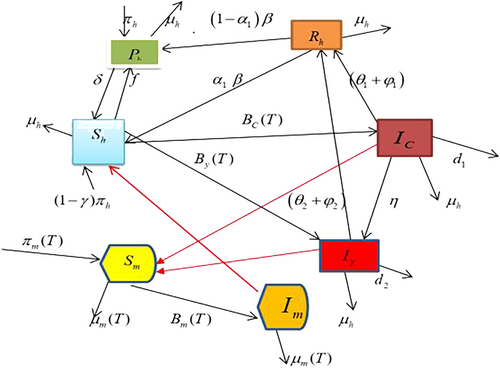
Figure 1 employs red lines to show how disease spreads and solid black lines to show how people or mosquitoes migrate across compartments. The dynamics of the disease were mirrored in the following nonautonomous deterministic system of nonlinear differential equations, which was based on the flow diagram and the assumptions mentioned above
d S h dt = ( 1 γ ) π h + δ P h + β α 1 R h f + B c ( T ) + B y ( T ) + μ h S h , d P h dt = γ π h + f S h + 1 α 1 β R h δ + μ h P h , d I c dt = B c ( T ) S h d 1 + μ h + η + θ 1 + φ 1 I c , d I y dt = B y ( T ) S h + η I c d 1 + μ h + θ 2 + φ 2 I y , dR dt = θ 2 + φ 2 I y + θ 1 + φ 1 I c β α 1 + 1 α 1 β + μ h R h , d S m dt = π m ( T ) B m ( T ) + μ m ( T ) S m , d I m dt = B m ( T ) S m μ m ( T ) I m , $$ {\displaystyle \begin{array}{cc}& \frac{\ d{S}_h\ }{dt}=\left(1-\gamma \right){\pi}_h+\delta {P}_h+\beta {\alpha}_1{R}_h-\left(f+{B}_c(T)+{B}_y(T)+{\mu}_h\right){S}_h,\\ {}& \frac{d{P}_h}{dt}=\gamma {\pi}_h+f{S}_h+\left(1-{\alpha}_1\right)\beta {R}_h-\left(\delta +{\mu}_h\right){P}_h,\\ {}& \frac{d{I}_c}{dt}={B}_c(T){S}_h-\left({d}_1+{\mu}_h+\eta +\left({\theta}_1+{\varphi}_1\right)\right){I}_c,\\ {}& \frac{d{I}_y}{dt}={B}_y(T){S}_h+\eta {I}_c-\left({d}_1+{\mu}_h+\left({\theta}_2+{\varphi}_2\right)\right){I}_y,\\ {}& \frac{dR}{dt}=\left({\theta}_2+{\varphi}_2\right){I}_y+\left({\theta}_1+{\varphi}_1\right){I}_c-\left(\beta {\alpha}_1+\left(1-{\alpha}_1\right)\beta +{\mu}_h\right){R}_h,\\ {}& \frac{d{S}_m}{dt}={\pi}_m(T)-\left({B}_m(T)+{\mu}_m(T)\right){S}_m,\\ {}& \frac{d{I}_m}{dt}={B}_m(T){S}_m-{\mu}_m(T){I}_m,\end{array}} $$ (9)
where, B m = b 2 ( T ) ε c I c N h + b 2 ( T ) ε y I y N h , B c = b 1 ( T ) ε c I m N h , B y = b 1 ( T ) ε y I m N h , $$ {B}_m=\frac{b_2(T){\varepsilon}_c{I}_c}{N_h}+\frac{b_2(T){\varepsilon}_y{I}_y}{N_h},{B}_c=\frac{b_1(T)\ {\varepsilon}_c\ {I}_m}{N_h},{B}_y=\frac{b_1(T)\ {\varepsilon}_y\ {I}_m}{N_h}, $$ are the mosquito's potency of infection, pre-school age, and young age, respectively.
Details are in the caption following the image
Flow chart of malaria disease dynamics.
The corresponding Caputo fractional-order equations of classical-order malaria model dynamics are proposed as follows:
a C D t α S h ( t ) = ( 1 γ ) π h + δ P h + β α 1 R h f + B c ( T ) + B y ( T ) + μ h S h , a C D t α P h ( t ) = γ π h + f S h + 1 α 1 β R h δ + μ h P h , a C D t α I c ( t ) = B c ( T ) S h d 1 + μ h + η + θ 1 + φ 1 I c , a C D t α I y ( t ) = B y ( T ) S h + η I c d 1 + μ h + θ 2 + φ 2 I y , a C D t α R h ( t ) = θ 2 + φ 2 I y + θ 1 + φ 1 I c β α 1 + 1 α 1 β + μ h R h , a C D t α S m ( t ) = π m ( T ) B m ( T ) + μ m ( T ) S m , a C D t α I m ( t ) = B m ( T ) S m μ m ( T ) I m . $$ {\displaystyle \begin{array}{cc}& {}_a^C{D}_t^{\alpha }{S}_h(t)=\left(1-\gamma \right){\pi}_h+\delta {P}_h+\beta {\alpha}_1{R}_h-\left(f+{B}_c(T)+{B}_y(T)+{\mu}_h\right){S}_h,\\ {}& {}_a^C{D}_t^{\alpha }{P}_h(t)=\gamma {\pi}_h+f{S}_h+\left(1-{\alpha}_1\right)\beta {R}_h-\left(\delta +{\mu}_h\right){P}_h,\\ {}& {}_a^C{D}_t^{\alpha }{I}_c(t)={B}_c(T){S}_h-\left({d}_1+{\mu}_h+\eta +\left({\theta}_1+{\varphi}_1\right)\right){I}_c,\\ {}& {}_a^C{D}_t^{\alpha }{I}_y(t)={B}_y(T){S}_h+\eta {I}_c-\left({d}_1+{\mu}_h+\left({\theta}_2+{\varphi}_2\right)\right){I}_y,\\ {}& {}_a^C{D}_t^{\alpha }{R}_h(t)=\left({\theta}_2+{\varphi}_2\right){I}_y+\left({\theta}_1+{\varphi}_1\right){I}_c-\left(\beta {\alpha}_1+\left(1-{\alpha}_1\right)\beta +{\mu}_h\right){R}_{h,}\\ {}& {}_a^C{D}_t^{\alpha }{S}_m(t)={\pi}_m(T)-\left({B}_m(T)+{\mu}_m(T)\right){S}_m,\\ {}& {}_a^C{D}_t^{\alpha }{I}_m(t)={B}_m(T){S}_m-{\mu}_m(T){I}_m.\end{array}} $$ (10)

4 Fractional Model Analysis

The Caputo derivative described by the system of DEs, the mathematical model, can be written as:
a C D t α X ( t ) = F ( t , X ( t ) ) $$ {}_a^C{D}_t^{\alpha }X(t)=F\left(t,X(t)\right) $$ (11)
X ( t ) = S h ( t ) , P h ( t ) , I C ( t ) , I y ( t ) , R h ( t ) S m ( t ) , I m ( t ) $$ X(t)=\left({S}_h(t),{P}_h\ \left(\mathrm{t}\right),{I}_C(t),{I}_y(t),{R}_h(t){S}_m(t),{I}_m(t)\right) $$ (12)
where, in Equation (11), F i ( t , X ( t ) ) $$ {F}_i\left(t,X(t)\right) $$ for i = 1 , 2 , 3 , 4 , 5 , 6 , 7 $$ i=1,2,3,4,5,6,7 $$ are kernels of the flexible structure. With initial conditions,
S h ( 0 ) = S h 0 , P h ( 0 ) = P h 0 , I C ( 0 ) = I C 0 , I y ( 0 ) = I y 0 , S m ( 0 ) = S m 0 , I m ( t ) = I m 0 . $$ {S}_h(0)={S}_{h0},{P}_h(0)={P}_{h0},{I}_C(0)={I}_{C0},{I}_y(0)={I}_{y0},{S}_m(0)={S}_{m0},{I}_m(t)={I}_{m0}. $$ (13)

4.1 Existence, Uniqueness, and Positivity of the Solution

First, we write system (11) as follows:
a C D t α S h ( t ) = F 1 t , S h , a C D t α P h ( t ) = F 2 t , P h , a C D t α I c ( t ) = F 3 t , I c , a C D t α I y ( t ) = F 4 t , I y , a C D t α R h ( t ) = F 5 t , R h , a C D t α S m ( t ) = F 6 t , S m , a C D t α I m ( t ) = F 7 t , I m , $$ {\displaystyle \begin{array}{cc}& {}_a^C{D}_t^{\alpha }{S}_h(t)={\mathrm{F}}_1\left(t,{S}_h\right),\\ {}& {}_a^C{D}_t^{\alpha }{P}_h(t)={\mathrm{F}}_2\left(t,{P}_h\right),\\ {}& {}_a^C{D}_t^{\alpha }{I}_c(t)={\mathrm{F}}_3\left(t,{I}_c\right),\\ {}& {}_a^C{D}_t^{\alpha }{I}_y(t)={\mathrm{F}}_4\left(t,{I}_y\right),\\ {}& {}_a^C{D}_t^{\alpha }{R}_h(t)={\mathrm{F}}_5\left(t,{R}_h\right),\\ {}& {}_a^C{D}_t^{\alpha }{S}_m(t)={\mathrm{F}}_6\left(t,{S}_m\right),\\ {}& {}_a^C{D}_t^{\alpha }{I}_m(t)={\mathrm{F}}_7\left(t,{I}_m\right),\end{array}} $$ (14)
where, F i ( t , X ) $$ {F}_i\left(t,X\right) $$ are kernels for i = 1 , 2 , 3 , 4 , 5 , 6 , 7 $$ i=1,2,3,4,5,6,7 $$ , and X = S h ( t ) , P h ( t ) , I c ( t ) , I y ( t ) , R h ( t ) , S m ( t ) , I m ( t ) . $$ X={S}_h(t),{P}_h(t),{I}_c(t),{I}_y(t),{R}_h(t),{S}_m(t),{I}_m(t). $$

Theorem 4.1.Suppose B be the Banach space of continuous real-valued functions with the associated norm that is defined in interval I.

S h ( t ) , P h ( t ) , I C ( t ) , I y ( t ) , R h ( t ) S m ( t ) , I m ( t ) = S h + P h + I C + I y + R h + S m + I m $$ {\displaystyle \begin{array}{cc}& \left\Vert {S}_h(t),{P}_h\ \left(\mathrm{t}\right),{I}_C(t),{I}_y(t),{R}_h(t){S}_m(t),{I}_m(t)\right\Vert \\ {}& \kern1em =\left\Vert {S}_h+{P}_h+{I}_C+{I}_y+{R}_h+{S}_m+{I}_m\right\Vert \end{array}} $$ (15)

from (15) above, we have
S h = sup S h ( t ) : t I , P h = sup P h ( t ) : t I , I c = sup I c ( t ) : t I , I y = sup I y ( t ) : t I , R h = sup R h ( t ) : t I , S m = sup S m ( t ) : t I , I m = sup I m ( t ) : t I , $$ {\displaystyle \begin{array}{cc}& \left\Vert {S}_h\right\Vert =\mathit{\sup}\left\{\left|{S}_h(t)\right|:t\in I\right\},\\ {}& \left\Vert {P}_h\right\Vert =\mathit{\sup}\left\{\left|{P}_h(t)\right|:t\in I\right\},\\ {}& \left\Vert {I}_c\right\Vert =\mathit{\sup}\left\{\left|{I}_c(t)\right|:t\in I\right\},\\ {}& \left\Vert {I}_y\right\Vert =\mathit{\sup}\left\{\left|{I}_y(t)\right|:t\in I\right\},\\ {}& \left\Vert {R}_h\right\Vert =\mathit{\sup}\left\{\left|{R}_h(t)\right|:t\in I\right\},\\ {}& \left\Vert {S}_m\right\Vert =\mathit{\sup}\left\{\left|{S}_m(t)\right|:t\in I\right\},\\ {}& \left\Vert {I}_m\right\Vert =\mathit{\sup}\left\{\left|{I}_m(t)\right|:t\in I\right\},\end{array}} $$ (16)
Consider the set B = E $$ E $$ (J) × E $$ E $$ (J) × E $$ E $$ (J) × E $$ E $$ (J) × E $$ E $$ (J) × E $$ E $$ (J) × E $$ E $$ (J), where E $$ E $$ (J) = C[0,T] is the Banach space of real-valued continuous functions defined on an interval J = [0,T] with the corresponding norm defined by;
S h ( t ) , P h ( t ) , I C ( t ) , I y ( t ) , R h ( t ) S m ( t ) , I m ( t ) = S h + P h + I C + I y + R h + S m + I m $$ {\displaystyle \begin{array}{cc}& \left\Vert {S}_h(t),{P}_h\ \left(\mathrm{t}\right),{I}_C(t),{I}_y(t),{R}_h(t){S}_m(t),{I}_m(t)\right\Vert =\left\Vert {S}_h\right\Vert +\left\Vert {P}_h\right\Vert \\ {}& \kern1em +\left\Vert {I}_C\right\Vert +\left\Vert {I}_y\right\Vert +\left\Vert {R}_h\right\Vert +\left\Vert {S}_m\right\Vert +\left\Vert {I}_m\right\Vert \end{array}} $$ (17)
and the associated sup norm [48],
where the Banach region of actual values of continuous functions formed at the range J = C [ 0 , T ] , $$ J=C\left[0,T\right], $$ is denoted by F ( J ) = C [ 0 , T ] . $$ F(J)=C\left[0,T\right]. $$ Knowing whether a mathematical model exists and its unique solution is crucial for researchers in the natural sciences. We employed the Banach fixed point theorem to demonstrate the existence of the solution to the given model. We demonstrate the solution, existence, and uniqueness and thoroughly investigate fixed points and contractions, applying the Caputo fractional integral for the suggested model [49]. Thus, the system is stated as such:
X ( t ) X ( 0 ) = 1 Γ ( α ) 0 t F i ( τ , X ( τ ) ) ( t τ ) α 1 d τ , i = 1 , 2 , 3 , 4 , 5 , 6 , 7 $$ X(t)-X(0)=\frac{1}{\Gamma \left(\alpha \right)}{\int}_0^t{F}_i\left(\tau, X\left(\tau \right)\right){\left(t-\tau \right)}^{\alpha -1} d\tau, \mathrm{i}=1,2,3,4,5,6,7 $$ (18)
S h ( t ) S h ( 0 ) = 1 Γ ( α ) 0 t F 1 τ , S h ( t τ ) α 1 d τ , P h ( t ) P h ( 0 ) = 1 Γ ( α ) a t F 2 τ , P h ( t τ ) α 1 d τ , I C ( t ) I C ( 0 ) = 1 Γ ( α ) a t F 3 τ , I C ( t τ ) α 1 d τ , I y ( t ) I y ( 0 ) = 1 Γ ( α ) a t F 4 τ , I y ( t τ ) α 1 d τ , R h ( t ) R h ( 0 ) = 1 Γ ( α ) a t F 5 τ , R h ( t τ ) α 1 d τ , S m ( t ) S m ( 0 ) = 1 Γ ( α ) a t F 6 τ , S m ( t τ ) α 1 d τ , $$ {\displaystyle \begin{array}{cc}& {S}_h(t)-{S}_h(0)=\frac{1}{\varGamma \left(\alpha \right)}{\int}_0^t{F}_1\left(\tau, {S}_h\right){\left(t-\tau \right)}^{\alpha -1} d\tau, \\ {}& {P}_h(t)-{P}_h(0)=\frac{1}{\varGamma \left(\alpha \right)}{\int}_a^t{F}_2\left(\tau, {P}_h\right){\left(t-\tau \right)}^{\alpha -1} d\tau, \\ {}& {I}_C(t)-{I}_C(0)=\frac{1}{\varGamma \left(\alpha \right)}{\int}_a^t{F}_3\left(\tau, {I}_C\right){\left(t-\tau \right)}^{\alpha -1} d\tau, \\ {}& {I}_y(t)-{I}_y(0)=\frac{1}{\varGamma \left(\alpha \right)}{\int}_a^t{F}_4\left(\tau, {I}_y\right){\left(t-\tau \right)}^{\alpha -1} d\tau, \\ {}& {R}_h(t)-{R}_h(0)=\frac{1}{\varGamma \left(\alpha \right)}{\int}_a^t{F}_5\left(\tau, {R}_h\right){\left(t-\tau \right)}^{\alpha -1} d\tau, \\ {}& {S}_m(t)-{S}_m(0)=\frac{1}{\varGamma \left(\alpha \right)}{\int}_a^t{F}_6\left(\tau, {S}_m\right){\left(t-\tau \right)}^{\alpha -1} d\tau, \end{array}} $$ (19)

Theorem 4.2.(Lipchitz condition and contraction) in [48] with the kernel F i , i = 1 , 2 , 3 , 4 , 5 , 6 , 7 $$ {F}_i,i=1,2,3,4,5,6,7 $$ fulfill the Lipschitz requirement and contraction if an inequality given below hold L i > 0 , i = 1 , 2 , 3 , 4 , 5 , 6 , 7 $$ {L}_i>0,i=1,2,3,4,5,6,7 $$ such that:

F i ( t , X ( t ) ) F i t , X 1 ( t ) L i X ( t ) X 1 ( t ) , F 1 t , S h F 1 t , S h 1 ( t ) L 1 S h S h 1 ( t ) , F 2 t , P h F 2 t , P h 1 ( t ) L 2 P h P h 1 ( t ) , F 3 t , I C F 3 t , I C 1 ( t ) L 3 I C I C 1 ( t ) , F 4 t , I y F 4 t , I y 1 ( t ) L 4 I y I y 1 ( t ) , F 5 t , R h F 5 t , R h 1 ( t ) L 5 R h R h 1 ( t ) , F 6 t , S m F 6 t , S m 1 ( t ) L 6 S m S m 1 ( t ) , F 7 t , I m F 6 t , I m 1 ( t ) L 7 I m I m 1 ( t ) , $$ {\displaystyle \begin{array}{cc}& \left\Vert {F}_i\Big(t,X(t)\Big)-{F}_i\left(t,{X}_1(t)\right)\right\Vert \le {L}_i\left\Vert X(t)-{X}_1(t)\right\Vert, \\ {}& \left\Vert {F}_1\left(t,{S}_h\right)-{F}_1\left(t,{S}_{h1}(t)\right)\right\Vert \le {L}_1\left\Vert {S}_h-{S}_{h1}(t)\right\Vert, \\ {}& \left\Vert {F}_2\left(t,{P}_h\right)-{F}_2\left(t,{P}_{h1}(t)\right)\right\Vert \le {L}_2\left\Vert {P}_h-{P}_{h1}(t)\right\Vert, \\ {}& \left\Vert {F}_3\left(t,{I}_C\right)-{F}_3\left(t,{I}_{C1}(t)\right)\right\Vert \le {L}_3\left\Vert {I}_C-{I}_{C1}(t)\right\Vert, \\ {}& \left\Vert {F}_4\left(t,{I}_y\right)-{F}_4\left(t,{I}_{y1}(t)\right)\right\Vert \le {L}_4\left\Vert {I}_y-{I}_{y1}(t)\right\Vert, \\ {}& \left\Vert {F}_5\left(t,{R}_h\right)-{F}_5\left(t,{R}_{h1}(t)\right)\right\Vert \le {L}_5\left\Vert {R}_h-{R}_{h1}(t)\right\Vert, \\ {}& \left\Vert {F}_6\left(t,{S}_m\right)-{F}_6\left(t,{S}_{m1}(t)\right)\right\Vert \le {L}_6\left\Vert {S}_m-{S}_{m1}(t)\right\Vert, \\ {}& \left\Vert {F}_7\left(t,{I}_m\right)-{F}_6\left(t,{I}_{m1}(t)\right)\right\Vert \le {L}_7\left\Vert {I}_m-{I}_{m1}(t)\right\Vert, \end{array}} $$ (20)

are contractions for 0 L i < 1 , $$ 0\le {\mathrm{L}}_{\mathrm{i}}<1, $$ .

Proof. Let the kernel F 1 $$ {F}_1 $$ fulfill the Lipschitz requirement and contraction if an inequality given below is hold,
0 f + μ h + b 1 ε c N h + b 1 ε y N h < 1 $$ 0\le f+{\mu}_h+\frac{b_1\ {\varepsilon}_c\ }{N_h}+\frac{b_1\ {\varepsilon}_y\ }{N_h}<1 $$ (21)
F 1 t , S h F 1 t , S h 1 ( t ) = ( 1 γ ) π h + δ P h + β α 1 R h f + μ h + b 1 ε c N h + b 1 ε y N h I m S h ( 1 γ ) π h + δ P h + β α 1 R h f + μ h + b 1 ε c N h + b 1 ε y N h I m S h 1 $$ \left\Vert {F}_1\left(t,{S}_h\right)-{F}_1\left(t,{S}_{h1}(t)\right)\right\Vert =\left\Vert \begin{array}{l}\left(1-\gamma \right){\pi}_h+\delta {P}_h+\beta {\alpha}_1{R}_h\\ {}-\left(f+{\mu}_h+\left(\frac{b_1\ {\varepsilon}_c\ }{N_h}+\frac{b_1\ {\varepsilon}_y\ }{N_h}\right){I}_m\right){S}_h-\\ {}\left(\left(1-\gamma \right){\pi}_h+\delta {P}_h+\beta {\alpha}_1{R}_h\right.\\ {}\left.-\left(f+{\mu}_h+\left(\frac{b_1\ {\varepsilon}_c\ }{N_h}+\frac{b_1\ {\varepsilon}_y\ }{N_h}\right){I}_m\right){S}_{h1}\right)\end{array}\right\Vert $$
= f + μ h + b 1 ε c N h + b 1 ε y N h S h 1 S h f + μ h + b 1 ε c N h + b 1 ε y N h Z 7 S h 1 S h L 1 ( S h 1 ) S h $$ {\displaystyle \begin{array}{cc}& =\left\Vert \left(f+{\mu}_h+\left(\frac{b_1\ {\varepsilon}_c\ }{N_h}+\frac{b_1\ {\varepsilon}_y\ }{N_h}\right)\left({S}_{h1}-{S}_h\right)\right)\right\Vert \\ {}& \kern1em \le \left\Vert \left(f+{\mu}_h+\left(\frac{b_1\ {\varepsilon}_c\ }{N_h}+\frac{b_1\ {\varepsilon}_y\ }{N_h}\right){Z}_7\left({S}_{h1}-{S}_h\right)\right)\le {L}_1\left({S}_{h1}\right)-{S}_h\right\Vert \end{array}} $$
such that, L 1 = f + μ h + b 1 ε c M N h + b 1 ε y M N h Z 7 , $$ {L}_1=f+{\mu}_h+\left(\frac{b_1\ {\varepsilon}_c\ }{M\left({N}_h\right)}+\frac{b_1\ {\varepsilon}_y\ }{M\left({N}_h\right)}\right){Z}_7, $$
where,
S h = Sup t J S h ( t ) = Z 1 , P h = Sup t J P h ( t ) = Z 2 $$ \left\Vert {S}_h\right\Vert =\underset{t\in J}{\mathrm{Sup}}\left\Vert {S}_h(t)\right\Vert ={Z}_1,\left\Vert {P}_h\right\Vert =\underset{t\in J}{\mathrm{Sup}}\left\Vert {P}_h(t)\right\Vert ={Z}_2 $$
I c = Sup t J I c ( t ) = Z 3 , I y = Sup t J I y ( t ) = Z 4 $$ \left\Vert {I}_c\right\Vert =\underset{t\in J}{\mathrm{Sup}}\left\Vert {I}_c(t)\right\Vert ={Z}_3,\left\Vert {I}_y\right\Vert =\underset{t\in J}{\mathrm{Sup}}\left\Vert {I}_y(t)\right\Vert ={Z}_4 $$
R h = Sup t J R h ( t ) = Z 5 , S m = Sup t J R m ( t ) = Z 6 , I m = Sup t J I m ( t ) = Z 7 $$ \left\Vert {R}_h\right\Vert =\underset{t\in J}{\mathrm{Sup}}\left\Vert {R}_h(t)\right\Vert ={Z}_5,\left\Vert {S}_m\right\Vert =\underset{t\in J}{\mathrm{Sup}}\left\Vert {R}_m(t)\right\Vert ={Z}_6,\left\Vert {I}_m\right\Vert =\underset{t\in J}{\mathrm{Sup}}\left\Vert {I}_m(t)\right\Vert ={Z}_7 $$
is enclosed, such that:
F 1 t , S h F 1 t , S h 1 L 1 S h S h 1 ( t ) $$ \left\Vert {F}_1\left(t,{S}_h\right)-{F}_1\left(t,{S}_{h1}\right)\right\Vert \le {L}_1\left\Vert {S}_h-{S}_{h1}(t)\right\Vert $$
thus for F 1 $$ {F}_1 $$ the Lipchitz condition obtained and if
0 τ + μ h + b 1 ε c N h + b 1 ε y N h Z 7 < 1 $$ \kern0.5em 0\le \tau +{\mu}_h+\left(\frac{b_1\ {\varepsilon}_c\ }{N_h}+\frac{b_1\ {\varepsilon}_y\ }{N_h}\right){Z}_7<1 $$ (22)
thus F 1 $$ {F}_1 $$ is contraction. Similarly for.

L 2 = δ + μ h , L 3 = d 1 + μ h + η + θ 1 + φ 1 L 4 = d 1 + μ h + ( θ 2 + φ 2 ) , $$ {L}_2=\left(\delta +{\mu}_h\right),{L}_3=\left({d}_1+{\mu}_h+\eta +\left({\theta}_1+{\varphi}_1\right)\right){L}_4={d}_1+{\mu}_h+\left({\theta}_2+{\varphi}_2\right), $$ L 5 = β α 1 + 1 α 1 β + μ h , L 6 = b 2 ε m z 3 + z 4 N h + μ m , L 7 = μ m , $$ {L}_5={\beta \alpha}_1+\left(1-{\alpha}_1\right)\beta +{\mu}_h,{L}_6=\frac{{\mathrm{b}}_2\ {\varepsilon}_m\left({z}_3+{z}_4\right)}{N_h}+{\mu}_m,{L}_7={\mu}_m, $$ are enclosed. If 0 L i < 1 , $$ 0\le {L}_i<1, $$ then F i , i = 2 , 3 , 4 , 5 , 6 , 7 $$ {F}_i,i=2,3,4,5,6,7 $$ are contractions.

Now for any positive integer n $$ n $$ we construct a recursive formula
X n ( t ) = 1 Γ ( α ) t 0 t F τ , X n 1 ( τ ) ( t τ ) α 1 d τ $$ {X}_n(t)=\frac{1}{\Gamma \left(\alpha \right)}{\int}_{t_0}^tF\left(\tau, {X}_{n-1}\left(\tau \right)\right){\left(t-\tau \right)}^{\alpha -1} d\tau $$ (23)
we adopt a recursive formula to convey the distinction between the consecutive terms, as mentioned in (19). According to Theorem (4.2), all kernels satisfy the Lipschitz condition.
A n ( t ) = X n ( t ) X n 1 ( t ) = 1 Γ ( α ) t 0 t F i τ X n 1 ( τ ) F i ( τ , X n 2 ( τ ) ( t τ ) α 1 d τ $$ {A}_n(t)={X}_n(t)-{X}_{n-1}(t)=\frac{1}{\Gamma \left(\alpha \right)}{\int}_{t_0}^t\left({F}_i\left(\tau {X}_{n-1}\left(\tau \right)\right)-{F}_i\Big(\tau, {X}_{n-2}\left(\tau \right)\right){\left(t-\tau \right)}^{\alpha -1} d\tau $$ (24)
A n ( t ) 1 Γ ( α ) F i t X n 1 ( t ) F i ) t , X n 2 ) ( t ) t t 0 α d τ $$ \left\Vert {A}_n(t)\right\Vert \le \frac{1}{\Gamma \left(\alpha \right)}\left\Vert {F}_i\left(t{X}_{n-1}(t)\right)-{F}_i\Big)t,{X}_{n-2}\Big)(t)\right\Vert {\left(t-{t}_0\right)}^{\alpha } d\tau $$ (25)
let us see the existence of the solution according to the general idea (20) and (21) with initial conditions:
S h 0 = S h ( 0 ) , P h 0 = P h ( 0 ) , I C 0 = I C ( 0 ) , I y 0 = I y ( 0 ) , R h 0 = R h ( 0 ) , S m 0 = S m ( 0 ) , I m 0 = I m ( 0 ) $$ {\displaystyle \begin{array}{cc}& {S}_{h0}={S}_h(0),{P}_{h0}={P}_h(0),{I}_{C0}={I}_C(0),{I}_{y0}={I}_y(0),{R}_{h0}={R}_h(0),\\ {}& \kern0em {S}_{m0}={S}_m(0),{I}_{m0}={I}_m(0)\end{array}} $$
the distinction between the consecutive terms is described below
A 1 n ( t ) = S hn ( t ) S hn 1 ( t ) = 1 Γ ( α ) t 0 t F 1 τ , S hn 1 ( τ ) F 1 ( τ , S hn 2 ( τ ) ( t τ ) α 1 d τ , A 2 n ( t ) = P hn ( t ) P hn 1 ( t ) = 1 Γ ( α ) t 0 t F 1 τ , P hn 1 ( τ ) F 1 ( τ , P hn 2 ( τ ) ( t τ ) α 1 d τ , A 3 n ( t ) = I Cn ( t ) S Cn 1 ( t ) = 1 Γ ( α ) t 0 t F 1 τ , I Cn 1 ( τ ) F 1 ( τ , I Cn 2 ( τ ) ( t τ ) α 1 d τ , A 4 n ( t ) = I yn ( t ) I yn 1 ( t ) = 1 Γ ( α ) t 0 t F 1 τ , I yn 1 ( τ ) F 1 ( τ , I yn 2 ( τ ) ( t τ ) α 1 d τ , A 5 n ( t ) = R hn ( t ) R hn 1 ( t ) = 1 Γ ( α ) t 0 t F 1 τ , R hn 1 ( τ ) F 1 ( τ , R hn 2 ( τ ) ( t τ ) α 1 d τ , A 6 n ( t ) = S mn ( t ) S mn 1 ( t ) = 1 Γ ( α ) t 0 t F 1 τ , S mn 1 ( τ ) F 1 ( τ , S mn 2 ( τ ) ( t τ ) α 1 d τ , A 7 n ( t ) = I mn ( t ) I mn 1 ( t ) = 1 Γ ( α ) t 0 t F 1 τ , I mn 1 ( τ ) F 1 ( τ , I mn 2 ( τ ) ( t τ ) α 1 d τ , $$ {\displaystyle \begin{array}{cc}& {A}_{1n}(t)={S}_{hn}(t)-{S}_{hn-1}(t)=\frac{1}{\Gamma \left(\alpha \right)}{\int}_{t_0}^t\left(\begin{array}{c}{F}_1\left(\tau, {S}_{hn-1}\left(\tau \right)\right)\\ {}-{F}_1\Big(\tau, {S}_{hn-2}\left(\tau \right)\end{array}\right){\left(t-\tau \right)}^{\alpha -1} d\tau, \\ {}& {A}_{2n}(t)={P}_{hn}(t)-{P}_{hn-1}(t)=\frac{1}{\Gamma \left(\alpha \right)}{\int}_{t_0}^t\left(\begin{array}{c}{F}_1\left(\tau, {P}_{hn-1}\left(\tau \right)\right)\\ {}-{F}_1\Big(\tau, {P}_{hn-2}\left(\tau \right)\end{array}\right){\left(t-\tau \right)}^{\alpha -1} d\tau, \\ {}& {A}_{3n}(t)={I}_{Cn}(t)-{S}_{Cn-1}(t)=\frac{1}{\Gamma \left(\alpha \right)}{\int}_{t_0}^t\left(\begin{array}{c}{F}_1\left(\tau, {I}_{Cn-1}\left(\tau \right)\right)\\ {}-{F}_1\Big(\tau, {I}_{Cn-2}\left(\tau \right)\end{array}\right){\left(t-\tau \right)}^{\alpha -1} d\tau, \\ {}& {A}_{4n}(t)={I}_{yn}(t)-{I}_{yn-1}(t)=\frac{1}{\Gamma \left(\alpha \right)}{\int}_{t_0}^t\left(\begin{array}{c}{F}_1\left(\tau, {I}_{yn-1}\left(\tau \right)\right)\\ {}-{F}_1\Big(\tau, {I}_{yn-2}\left(\tau \right)\end{array}\right){\left(t-\tau \right)}^{\alpha -1} d\tau, \\ {}& {A}_{5n}(t)={R}_{hn}(t)-{R}_{hn-1}(t)=\frac{1}{\Gamma \left(\alpha \right)}{\int}_{t_0}^t\left(\begin{array}{c}{F}_1\left(\tau, {R}_{hn-1}\left(\tau \right)\right)\\ {}-{F}_1\Big(\tau, {R}_{hn-2}\left(\tau \right)\end{array}\right){\left(t-\tau \right)}^{\alpha -1} d\tau, \\ {}& {A}_{6n}(t)={S}_{mn}(t)-{S}_{mn-1}(t)=\frac{1}{\Gamma \left(\alpha \right)}{\int}_{t_0}^t\left(\begin{array}{c}{F}_1\left(\tau, {S}_{mn-1}\left(\tau \right)\right)\\ {}-{F}_1\Big(\tau, {S}_{mn-2}\left(\tau \right)\end{array}\right){\left(t-\tau \right)}^{\alpha -1} d\tau, \\ {}& {A}_{7n}(t)={I}_{mn}(t)-{I}_{mn-1}(t)=\frac{1}{\Gamma \left(\alpha \right)}{\int}_{t_0}^t\left(\begin{array}{c}{F}_1\left(\tau, {I}_{mn-1}\left(\tau \right)\right)\\ {}-{F}_1\Big(\tau, {I}_{mn-2}\left(\tau \right)\end{array}\right){\left(t-\tau \right)}^{\alpha -1} d\tau, \end{array}} $$ (26)
consider the first equation of (26), and apply Theorem (4.2),
F i ( t , X ( t ) ) F i t , X 1 ( t ) L i X ( t ) X 1 ( t ) $$ \left\Vert {F}_i\Big(t,X(t)\Big)-{F}_i\left(t,{X}_1(t)\right)\right\Vert \le {L}_i\left\Vert X(t)-{X}_1(t)\right\Vert $$ (27)
and by applying the triangular inequality,
A 1 n ( t ) = S hn ( t ) S hn 1 ( t ) α Γ ( α ) L 1 S hn 1 S hn 2 t 0 t ( t τ ) α 1 d τ t α α Γ ( α ) L 1 S hn 1 S hn 2 , $$ {\displaystyle \begin{array}{cc}\left\Vert {A}_{1n}(t)\right\Vert & =\left\Vert {S}_{hn}(t)-{S}_{hn-1}(t)\right\Vert \le \frac{\alpha }{\Gamma \left(\alpha \right)}\left\Vert {L}_1{S}_{hn-1}-{S}_{hn-2}\right\Vert {\int}_{t_0}^t{\left(t-\tau \right)}^{\alpha -1} d\tau \\ {}& \le \frac{t^{\alpha }}{\alpha \Gamma \left(\alpha \right)}{L}_1\left\Vert {S}_{hn-1}-{S}_{hn-2}\right\Vert, \end{array}} $$
such that,
A 1 n ( t ) L 1 A 1 n 1 ( t ) t α α Γ ( α ) $$ \left\Vert {A}_{1n}(t)\right\Vert \le {L}_1\left\Vert {A}_{1n-1}(t)\right\Vert \left(\frac{t^{\alpha }}{\alpha \Gamma \left(\alpha \right)}\right) $$ (28)
by considering the second equation of (26),
A 2 n ( t ) = P hn ( t ) P hn 1 ( t ) α α Γ ( α ) L 1 P hn 1 P hn 2 t 0 t ( t τ ) α 1 d τ $$ \left\Vert {A}_{2n}(t)\right\Vert =\left\Vert {P}_{hn}(t)-{P}_{hn-1}(t)\right\Vert \le \frac{\alpha }{\alpha \Gamma \left(\alpha \right)}{L}_1\left\Vert {P}_{hn-1}-{P}_{hn-2}\right\Vert {\int}_{t_0}^t{\left(t-\tau \right)}^{\alpha -1} d\tau $$
t α α Γ ( α ) L 1 P hn 1 P hn 2 $$ \le \frac{t^{\alpha }}{\alpha \Gamma \left(\alpha \right)}{L}_1\left\Vert {P}_{hn-1}-{P}_{hn-2}\right\Vert $$
such that,
A 2 n ( t ) L 2 A 2 n 1 ( t ) t α α Γ ( α ) $$ \left\Vert {A}_{2n}(t)\right\Vert \le {L}_2\left\Vert {A}_{2n-1}(t)\right\Vert \left(\frac{t^{\alpha }}{\alpha \Gamma \left(\alpha \right)}\right) $$ (29)
similarly, the remaining expressions can be reduced to
A 3 n ( t ) L 3 A 3 n 1 ( t ) t α α Γ ( α ) , A 4 n ( t ) L 4 A 4 n 1 ( t ) t α α Γ ( α ) , A 5 n ( t ) L 5 A 5 n 1 ( t ) t α α Γ ( α ) , A 6 n ( t ) L 6 A 6 n 1 ( t ) t α α Γ ( α ) , A 7 n ( t ) L 7 A 7 n 1 ( t ) t α α Γ ( α ) . $$ {\displaystyle \begin{array}{c}\left\Vert {A}_{3n}(t)\right\Vert \le {L}_3\left\Vert {A}_{3n-1}(t)\right\Vert \left(\frac{t^{\alpha }}{\alpha \Gamma \left(\alpha \right)}\right),\\ {}\left\Vert {A}_{4n}(t)\right\Vert \le {L}_4\left\Vert {A}_{4n-1}(t)\right\Vert \left(\frac{t^{\alpha }}{\alpha \Gamma \left(\alpha \right)}\right),\\ {}\left\Vert {A}_{5n}(t)\right\Vert \le {L}_5\left\Vert {A}_{5n-1}(t)\right\Vert \left(\frac{t^{\alpha }}{\alpha \Gamma \left(\alpha \right)}\right),\\ {}\left\Vert {A}_{6n}(t)\right\Vert \le {L}_6\left\Vert {A}_{6n-1}(t)\right\Vert \left(\frac{t^{\alpha }}{\alpha \Gamma \left(\alpha \right)}\right),\\ {}\left\Vert {A}_{7n}(t)\right\Vert \le {L}_7\left\Vert {A}_{7n-1}(t)\right\Vert \left(\frac{t^{\alpha }}{\alpha \Gamma \left(\alpha \right)}\right).\end{array}} $$ (30)

Theorem 4.3.The Caputo fractional Mathematical model given in (10) has the solution, if there exists y 0 $$ {\mathrm{y}}_0 $$ such that:

y 0 α α Γ ( α ) L i < 1 , i = 1 , 2 , 3 , 4 , 5 , 6 , 7 $$ \left(\frac{{y_0}^{\alpha }}{\alpha \Gamma \left(\alpha \right)}\right){L}_i<1,i=1,2,3,4,5,6,7 $$ (31)

Proof. Using the recursive formula approaches, we obtain,
A 1 n ( t ) S h ( 0 ) L 1 y 0 α α Γ ( α ) n , A 2 n ( t ) P h ( 0 ) L 2 y 0 α α Γ ( α ) n , A 3 n ( t ) I c ( 0 ) L 3 y 0 α α Γ ( α ) n , A 4 n ( t ) I y ( 0 ) L 4 y 0 α α Γ ( α ) n , A 5 n ( t ) R h ( 0 ) L 5 y 0 α α Γ ( α ) n , A 6 n ( t ) S m ( 0 ) L 6 y 0 α α Γ ( α ) n , A 7 n ( t ) I m ( 0 ) L 7 y 0 α α Γ ( α ) n . $$ {\displaystyle \begin{array}{c}\left\Vert {A}_{1n}(t)\right\Vert \le \left\Vert {S}_h(0)\right\Vert\ {L}_1{\left(\frac{{y_0}^{\alpha }}{\alpha \Gamma \left(\alpha \right)}\right)}^n,\\ {}\left\Vert {A}_{2n}(t)\right\Vert \le \left\Vert {P}_h(0)\right\Vert\ {L}_2{\left(\frac{{y_0}^{\alpha }}{\alpha \Gamma \left(\alpha \right)}\right)}^n,\\ {}\left\Vert {A}_{3n}(t)\right\Vert \le \left\Vert {I}_c(0)\right\Vert\ {L}_3{\left(\frac{{y_0}^{\alpha }}{\alpha \Gamma \left(\alpha \right)}\right)}^n,\\ {}\left\Vert {A}_{4n}(t)\right\Vert \le \left\Vert {I}_y(0)\right\Vert\ {L}_4{\left(\frac{{y_0}^{\alpha }}{\alpha \Gamma \left(\alpha \right)}\right)}^n,\\ {}\left\Vert {A}_{5n}(t)\right\Vert \le \left\Vert {R}_h(0)\right\Vert\ {L}_5{\left(\frac{{y_0}^{\alpha }}{\alpha \Gamma \left(\alpha \right)}\right)}^n,\\ {}\left\Vert {A}_{6n}(t)\right\Vert \le \left\Vert {S}_m(0)\right\Vert\ {L}_6{\left(\frac{{y_0}^{\alpha }}{\alpha \Gamma \left(\alpha \right)}\right)}^n,\\ {}\left\Vert {A}_{7n}(t)\right\Vert \le \left\Vert {I}_m(0)\right\Vert\ {L}_7{\left(\frac{{y_0}^{\alpha }}{\alpha \Gamma \left(\alpha \right)}\right)}^n.\end{array}} $$ (32)
The presence of the solution of the mathematical model in (10) assured the theorem of Lipschitz condition and contraction above; now the functions
S h ( t ) , P h ( t ) , I c ( t ) , I y ( t ) , R h ( t ) , S m ( t ) , I m ( t ) $$ {S}_h(t),{P}_h(t),{I}_c(t),{I}_y(t),{R}_h(t),{S}_m(t),{I}_m(t) $$
are solutions of the mathematical model.

The existence of the solution of the mathematical model (10) is assured by the Theorem (4.2) and (32).

Now, we are going to show functions which S h ( t ) , P h ( t ) , I C ( t ) , I y ( t ) , R h ( t ) , S m ( t ) , I m ( t ) $$ {S}_h(t),\kern0.75em {P}_h(t),\kern0.5em {I}_C(t),\kern0.5em {I}_y(t),\kern0.5em {R}_h(t),\kern0.5em {S}_m(t),\kern0.5em {I}_m(t) $$ are the solutions of (10). By considering Equation (26),
a 1 n ( t ) 1 α Γ ( α ) 0 t F 1 k S hn 1 ( k ) F 1 ( k , S hn 2 ( k ) ) ( t k ) α 1 dk $$ \left\Vert {a}_{1n}(t)\right\Vert \le \frac{1}{\alpha \Gamma \left(\alpha \right)}{\int}_0^t\left\Vert \left({F}_1\left(k{S}_{hn-1}(k)\right)-{F}_1\Big(k,{S}_{hn-2}(k)\right)\right\Vert \Big){\left(t-k\right)}^{\alpha -1} dk $$
t α α Γ ( α ) L 1 S hn S hn 1 $$ \le \frac{t^{\alpha }}{\alpha \Gamma \left(\alpha \right)}{L}_1\left\Vert {S}_{hn}-{S}_{hn-1}\right\Vert $$
by repeating the process of the recursive formula, we obtain,
a 1 n ( t ) t α α Γ ( α ) n + 1 L 1 S hn S hn 1 n $$ \left\Vert {a}_{1n}(t)\right\Vert \le {\left[\frac{t^{\alpha }}{\alpha \Gamma \left(\alpha \right)}\right]}^{n+1}{\left({L}_1\ \left\Vert {S}_{hn}-{S}_{hn-1}\right\Vert \right)}^n $$
for t = y 0 , $$ t={y}_0, $$
a 1 n ( t ) y 0 α α Γ ( α ) n + 1 L 1 S hn S hn 1 n $$ \left\Vert {a}_{1n}(t)\right\Vert \le {\left[\frac{{y_0}^{\alpha }}{\alpha \Gamma \left(\alpha \right)}\right]}^{n+1}{\left({L}_1\ \left\Vert {S}_{hn}-{S}_{hn-1}\right\Vert \right)}^n $$
after some steps we obtain:
t α α Γ ( α ) L 1 < 1 $$ \left(\frac{t^{\alpha }}{\alpha \Gamma \left(\alpha \right)}\right){L}_1<1 $$
in similar way a in ( t ) 0 $$ \left\Vert {a}_{in}(t)\right\Vert \to 0 $$ , i = 2 , 3 , 4 , 5 , 6 , 7 , $$ i=2,3,4,5,6,7, $$ for t α α Γ ( α ) L i < 1 . $$ \left(\frac{t^{\alpha }}{\alpha \Gamma \left(\alpha \right)}\right){L}_i<1. $$ then the mathematical model system (10) has a solution.

Theorem 4.4.The Caputo fractional model (10) has a unique solution if

t α α Γ ( α ) L i < 1 , i = 1 , 2 , 3 , 4 , 5 , 6 , 7 . $$ \left(\frac{t^{\alpha }}{\alpha \Gamma \left(\alpha \right)}\right){L}_i<1,i=1,2,3,4,5,6,7. $$

Let X * ( t ) = S h 1 , P h 1 , I C 1 , I y 1 , R h 1 , S m 1 , I m 1 $$ {X}^{\ast }(t)=\left({S}_{h1},{P}_{h1},{I}_{C1},{I}_{y1},{R}_{h1},{S}_{m1},{I}_{m1}\right) $$ is the solution of the proposed fractional model.
X ( t ) X * ( t ) = 1 α Γ ( α ) t 0 t F 1 ( τ X ( τ ) ) F 1 ( τ , X * ( τ ) ) ( t τ ) α 1 d τ $$ X(t)-{X}^{\ast }(t)=\frac{1}{\alpha \Gamma \left(\alpha \right)}{\int}_{t_0}^t\left({F}_1\left(\tau X\left(\tau \right)\right)-{F}_1\Big(\tau, {X}^{\ast}\left(\tau \right)\right)\Big){\left(t-\tau \right)}^{\alpha -1} d\tau $$ (33)
by taking the norm of both sides,
X ( t ) X * ( t ) = 1 α Γ ( α ) t 0 t F 1 ( τ X ( τ ) ) F 1 ( τ , X * ( τ ) , ) ( t τ ) α 1 d τ $$ \left\Vert X(t)-{X}^{\ast }(t)\right\Vert =\frac{1}{\alpha \Gamma \left(\alpha \right)}{\int}_{t_0}^t\left\Vert {F}_1\left(\tau X\left(\tau \right)\right)-{F}_1\Big(\tau, {X}^{\ast}\left(\tau \right),\Big)\right\Vert {\left(t-\tau \right)}^{\alpha -1} d\tau $$ (34)
Using the triangular inequality, we obtain,
X ( t ) X * ( t ) t α α Γ ( α ) L i X ( t ) X * ( t ) $$ \left\Vert X(t)-{X}^{\ast }(t)\right\Vert \le \frac{t^{\alpha }}{\alpha \Gamma \left(\alpha \right)}{L}_i\left\Vert X(t)-{X}^{\ast }(t)\right\Vert $$
X ( t ) X * ( t ) 1 t α α Γ ( α ) L i $$ \left\Vert X(t)-{X}^{\ast }(t)\right\Vert \left(1\le \frac{t^{\alpha }}{\alpha \Gamma \left(\alpha \right)}{L}_i\right) $$
1 t α α Γ ( α ) L i > 0 $$ \left(1-\frac{t^{\alpha }}{\alpha \Gamma \left(\alpha \right)}{L}_i\right)>0 $$
we obtain, 0 = X ( t ) X * ( t ) , X ( t ) = X * ( t ) $$ 0=\left\Vert X(t)-{X}^{\ast }(t)\right\Vert, X(t)={X}^{\ast }(t) $$ , so the proposed model has a unique solution. For sure, let us take the first compartment of (10),
S h ( t ) S h 1 ( t ) = 1 α Γ ( α ) t 0 t F 1 τ S h ( τ ) F 1 ( τ , S h 1 ( τ ) ( t τ ) α 1 d τ $$ {S}_h(t)-{S}_{h1}(t)=\frac{1}{\alpha \Gamma \left(\alpha \right)}{\int}_{t_0}^t\left({F}_1\left(\tau {S}_h\left(\tau \right)\right)-{F}_1\Big(\tau, {S}_{h1}\left(\tau \right)\right){\left(t-\tau \right)}^{\alpha -1} d\tau $$
by taking the norm of both sides,
S h ( t ) S h 1 ( t ) t α α Γ ( α ) L 1 S h ( t ) S h 1 ( t ) $$ \left\Vert {S}_h(t)-{S}_{h1}(t)\ \right\Vert \le \frac{t^{\alpha }}{\alpha \Gamma \left(\alpha \right)}{L}_1\left\Vert {S}_h(t)-{S}_{h1}(t)\right\Vert $$
S h ( t ) S h 1 ( t ) S h ( t ) S h 1 ( t ) L 1 t α α Γ ( α ) $$ \left\Vert {S}_h(t)-{S}_{h1}(t)\ \right\Vert \le \left\Vert {S}_h(t)-{S}_{h1}(t)\right\Vert\ {L}_1\frac{t^{\alpha }}{\alpha \Gamma \left(\alpha \right)} $$
S h ( t ) S h 1 ( t ) 1 t α α Γ ( α ) L 1 , $$ \left\Vert {S}_h(t)-{S}_{h1}(t)\ \right\Vert \left(1\le \frac{t^{\alpha }}{\alpha \Gamma \left(\alpha \right)}{L}_1\right), $$ after some steps, we obtain:
1 t α α Γ ( α ) L 1 > 0 $$ \left(1-\frac{t^{\alpha }}{\alpha \Gamma \left(\alpha \right)}{L}_1\right)>0 $$
for

S h ( t ) S h 1 ( t ) = 0 , $$ \kern5em \left\Vert {S}_h(t)-{S}_{h1}(t)\right\Vert =0, $$ thus S h ( t ) = S h 1 ( t ) , $$ {S}_h(t)={S}_{h1}(t), $$

so the proposed model has a unique solution.

Similarly,
S h ( t ) = S h 1 ( t ) , P h ( t ) = P h 1 ( t ) , I C ( t ) = I C 1 ( t ) , I y ( t ) = I y 1 ( t ) , R h ( t ) = R h 1 ( t ) , S m ( t ) = S m 1 ( t ) , I m ( t ) = I m 1 ( t ) . $$ {\displaystyle \begin{array}{cc}& {S}_h(t)={S}_{h1}(t),{P}_h(t)={P}_{h1}(t),{I}_C(t)={I}_{C1}(t),{I}_y(t)={I}_{y1}(t),\\ {}& {R}_h(t)={R}_{h1}(t),{S}_m(t)={S}_{m1}(t),{I}_m(t)={I}_{m1}(t).\end{array}} $$ (35)

From all of these, we determined that the suggested model has a unique solution and that the region of the investigation is epidemiologically feasible. If the solution of (10) without negative beginning data remains non-negative for all time, then the model will have epidemiological significance.

Theorem 4.5.Epidemiologically appropriate region of Caputo fractional model (10) is provided that:

M = S h ( t ) , P h ( t ) , I C ( t ) , I y ( t ) , R h ( t ) , S m ( t ) , I m ( t ) R + 7 0 S h ( t ) + P h ( t ) + I C ( t ) + I y ( t ) , R h ( t ) N h π h μ h 0 S m ( t ) + I m ( t ) N m π m μ m . $$ M=\left\{\begin{array}{l}{S}_h(t),{P}_h(t),{I}_C(t),{I}_y(t),{R}_h(t),{S}_m(t),{I}_m(t)\in {R_{+}}^7\\ {}\ 0\le {S}_h(t)+{P}_h(t)+{I}_C(t)+{I}_y(t),{R}_h(t)\le {N}_h\le \frac{\pi_h}{\mu_h}\\ {}0\le {S}_m(t)+{I}_m(t)\le {N}_m\le \frac{\pi_m}{\mu_m}\end{array}\right\}. $$

Lemma 4.1.(The generalized average value theorem) [30] let f ( x ) C [ a , b ] $$ f(x)\in C\left[a,b\right] $$ and let D t α 0 C f ( x ) $$ {}_0{}^CD_t^{\alpha }f(x) $$ 0 C [ a , b ] $$ \ge 0\in C\left[a,b\right] $$ when 0 < α 1 $$ 0<\alpha \le 1 $$ . Then we have

f ( x ) = f ( a ) + 1 Γ ( α ) D t α 0 C f ( ε ) ( x a ) α $$ f(x)=f(a)+\frac{1}{\Gamma \left(\alpha \right)}{}_0{}^CD_t^{\alpha }f\left(\varepsilon \right){\left(x-a\right)}^{\alpha } $$ , when 0 ε x , x ( a , b ] . $$ 0\le \varepsilon \le x,{\forall}_x\in \left(a,b\right]. $$

Now, by considering the above lemma, if
f ( x ) C [ 0 , b ] , D t α 0 C f ( x ) C [ a , b ] $$ f(x)\in C\left[0,b\right],{}_0{}^CD_t^{\alpha }f(x)\in C\left[a,b\right] $$
D t α 0 C f ( x ) 0 , x ( 0 , b ] $$ {}_0{}^CD_t^{\alpha }f(x)\ge 0,{\forall}_x\in \left(0,b\right] $$
if 0 < α 1 $$ 0<\alpha \le 1 $$ then, the function f ( x ) $$ f(x) $$ is non-decreasing and,

if D t α 0 C f ( x ) 0 $$ {}_0{}^CD_t^{\alpha }f(x)\le 0 $$ x ( 0 , b ] $$ {\forall}_x\in \left(0,b\right] $$ then, the function f ( x ) $$ f(x) $$ is non-increasing x ( 0 , b ] . $$ {\forall}_x\in \left(0,b\right]. $$

Let us demonstrate the positive invariance of M; from (11) we have,
D t α 0 C S h ( t ) S h = 0 = ( 1 γ ) π h + δ P h + β α 1 R h 0 , D t α 0 C P h ( t ) P h = 0 = γ π h + fS h + 1 α 1 β R h 0 . $$ {\displaystyle \begin{array}{c}{}_0{}^CD_t^{\alpha }{S}_h(t)\left|{S}_h=0\right.=\left(1-\gamma \right){\pi}_h+\delta {P}_h+{\beta \alpha}_1{R}_h\ge 0,\\ {}{}_0{}^CD_t^{\alpha }{P}_h(t)\left|{P}_h=0\right.={\gamma \pi}_h+{fS}_h+\left(1-{\alpha}_1\right)\beta {R}_h\ge 0.\end{array}} $$ (36)
In the same way, every last solution in the model is non-negative and stays in M. Additionally, we need to determine the fractional derivatives of the entire population by adding up all of the system relations to demonstrate that the solution is bounded.
D t α 0 C N h ( t ) = D t α 0 C S h ( t ) + D t α 0 C P h ( t ) + D t α 0 C I c ( t ) + D t α 0 C I y ( t ) + D t α 0 C R h ( t ) + D t α 0 C S m ( t ) + D t α 0 C I m ( t ) , D t α 0 C N h ( t ) π h μ h N h , D t α 0 C N h ( t ) + μ h N h π h , $$ {\displaystyle \begin{array}{cc}& {}_0{}^CD_t^{\alpha }{N}_h(t)={}_0{}^CD_t^{\alpha }{S}_h(t)+{}_0{}^CD_t^{\alpha }{P}_h(t)+{}_0{}^CD_t^{\alpha }{I}_c(t)+{}_0{}^CD_t^{\alpha }{I}_y(t)\\ {}& \kern1em +{}_0{}^CD_t^{\alpha }{R}_h(t)+{}_0{}^CD_t^{\alpha }{S}_m(t)+{}_0{}^CD_t^{\alpha }{I}_m(t),\\ {}& {}_0{}^CD_t^{\alpha }{N}_h(t)\le {\pi}_h-{\mu}_h{N}_h,\\ {}& {}_0{}^CD_t^{\alpha }{N}_h(t)+{\mu}_h{N}_h\le {\pi}_h,\end{array}} $$ (37)
by considering the Laplace transform of Caputo fractional-order derivatives of Theorem (2.1),
L [ D t α 0 C f ( t ) ] = S α F ( s ) k = 0 n 1 S α k 1 f ( k ) ( 0 ) $$ L\left[{}_0{}^CD_t^{\alpha }f(t)\right]={S}^{\alpha }F(s)-\sum \limits_{k=0}^{n-1}{S}^{\alpha -k-1}{f}^{(k)}(0) $$
using the Laplace transform of both sides of (27),
L D t α 0 C N h ( t ) + μ h N h L π h $$ L\left\{{}_0{}^CD_t^{\alpha }{N}_h(t)+{\mu}_h{N}_h\right\}\le L\left({\pi}_h\right) $$
by the linearity of the Laplace transform, we obtain,
L D t α 0 C N h ( t ) + μ h L N h L π h $$ L\left\{{}_0{}^CD_t^{\alpha }{N}_h(t)\right\}+{\mu}_hL\left\{{N}_h\right\}\le L\left({\pi}_h\right) $$
then we get, s α L N h ( t ) k = 0 n 1 s α k 1 N h ( k ) ( 0 ) + μ h L N h π h S , $$ {s}^{\alpha }L\left\{{N}_h(t)\right\}-\sum \limits_{k=0}^{n-1}{s}^{\alpha -k-1}{N_h}^{(k)}(0)+{\mu}_hL\left\{{N}_h\right\}\le \frac{\pi_h}{S}, $$
L N h ( t ) 1 + μ h s α π h S · 1 s α + k = 0 n 1 1 s k + 1 N h ( k ) ( 0 ) $$ L\left\{{N}_h(t)\right\}\left(1+\frac{\mu_h}{s^{\alpha }}\right)\le \frac{\pi_h}{S}\cdotp \frac{1}{s^{\alpha }}+\sum \limits_{k=0}^{n-1}\ \frac{1}{s^{k+1}}\kern0.75em {N_h}^{(k)}(0) $$
using the Taylor series expansion, we have
L N h ( t ) π h S · 1 s α 1 1 + μ h s α + k = 0 n 1 1 s k + 1 1 1 + μ h s α N h ( k ) ( 0 ) $$ L\left\{{N}_h(t)\right\}\le \frac{\pi_h}{S}\cdotp \frac{1}{s^{\alpha }}\ \left(\frac{1}{1+\frac{\mu_h}{s^{\alpha }}}\right)+\sum \limits_{k=0}^{n-1}\ \frac{1}{s^{k+1}}\ \left(\frac{1}{1+\frac{\mu_h}{s^{\alpha }}}\right)\kern0.5em {N_h}^{(k)}(0) $$
1 1 + μ h s α = n = 0 μ h s α n $$ \left(\frac{1}{1+\frac{\mu_h}{s^{\alpha }}}\right)=\sum \limits_{n=0}^{\infty }{\left(\frac{-{\mu}_h}{s^{\alpha }}\right)}^n $$
therefore,
L N h ( t ) π h S · 1 s α n = 0 μ h s α n + k = 0 n 1 1 s k + 1 n = 0 μ h s α n N h ( k ) ( 0 ) $$ L\left\{{N}_h(t)\right\}\le \frac{\pi_h}{S}\cdotp \frac{1}{s^{\alpha }}\ \sum \limits_{n=0}^{\infty }{\left(\frac{-{\mu}_h}{s^{\alpha }}\right)}^n+\sum \limits_{k=0}^{n-1}\ \frac{1}{s^{k+1}}\sum \limits_{n=0}^{\infty }{\left(\frac{-{\mu}_h}{s^{\alpha }}\right)}^n\kern0.5em {N_h}^{(k)}(0) $$ (38)
by taking the inverse of the Laplace transform of (38), we obtain
N h ( t ) π h n = 0 μ h t α n Γ ( α n + 1 ) + k = 0 n 1 n = 0 μ h t α n Γ ( α n + k + 1 ) t k N h ( k ) ( 0 ) $$ {N}_h(t)\le {\pi}_h\sum \limits_{n=0}^{\infty}\kern0.5em \frac{{\left(-{\mu}_h{t}^{\alpha}\right)}^n}{\Gamma \left(\alpha n+1\right)}+\sum \limits_{k=0}^{n-1}\ \sum \limits_{n=0}^{\infty}\kern0.5em \frac{{\left(-{\mu}_h{t}^{\alpha}\right)}^n}{\Gamma \left(\alpha n+k+1\right)}\kern0.5em {t}^k{N_h}^{(k)}(0) $$
after some steps, we obtain,
N h ( t ) π h E 1 μ h t α + k = 0 n 1 E k + 1 μ h t α t k N h ( k ) ( 0 ) $$ {N}_h(t)\le {\pi}_h{E}_1\left(-{\mu}_h{t}^{\alpha}\right)+\sum \limits_{k=0}^{n-1}\kern0.5em {E}_{k+1}\left(-{\mu}_h{t}^{\alpha}\right){t}^k{N_h}^{(k)}(0) $$ (39)
where E 1 μ h t α , E k + 1 μ h t α t k , $$ {E}_1\left(-{\mu}_h{t}^{\alpha}\right),{E}_{k+1}\left(-{\mu}_h{t}^{\alpha}\right){t}^k, $$ in (39) are series of functions which converge for any argument. Hence, the model is a biologically feasible region that means the total human population is bounded in similar way the total mosquito population is also bounded.

5 Equilibrium Points and Stability Analysis

5.1 Disease-Free Equilibrium (DFE) Point

At the DFE, all the disease classes are 0. It is a scenario that depicts an infection-free state in the community or society. The DFE of the model (10) is obtained by setting the right-hand side of the equation in the model equal to 0.

Furthermore, at DFE point ( ε 0 $$ {\varepsilon}_0 $$ ), I c = 0 , I y = 0 , I m = 0 $$ {I}_c=0,{I}_y=0,{I}_m=0 $$ , which is given by
ε 0 = S h 0 , P h 0 , 0 , 0 , R h 0 , S m 0 , 0 $$ {\varepsilon}_0=\left({S_h}^0,{P_h}^0,0,0,{R_h}^0,{S_m}^0,0\right) $$ (40)
To obtain DFE, set the right-hand side of the equation of the model (10) to 0.
For instance, consider the first equation of (10)
D t α a C S h ( t ) = ( 1 γ ) π h + δ P h + β α 1 R h f + B c ( T ) + B y ( T ) + μ h S h $$ {}_a{}^CD_t^{\alpha }{S}_h(t)=\left(1-\gamma \right){\pi}_h+\delta {P}_h+{\beta \alpha}_1{R}_h-\left(f+{B}_c(T)+{B}_y(T)+{\mu}_h\right){S}_h $$ (41)
( 1 γ ) π h + δ P h + β α 1 R h f + B c ( T ) + B y ( T ) + μ h S h = 0 $$ \left(1-\gamma \right){\pi}_h+\delta {P}_h+{\beta \alpha}_1{R}_h-\left(f+{B}_c(T)+{B}_y(T)+{\mu}_h\right){S}_h=0 $$
The force of infection for both age structures of humans is 0 such that,
B c = B y = 0 $$ {\mathrm{B}}_c={\mathrm{B}}_y=0 $$
by solving (40) for S h $$ {S}_h $$ and after some steps, we obtain:
S h 0 = δ + ( 1 γ ) μ h π h f + μ h + δ μ h $$ {S_h}^0=\frac{\left(\delta +\left(1-\gamma \right){\mu}_h\right){\pi}_h}{\left(f+{\mu}_h+\delta \right){\mu}_h} $$ (42)
similarly for D t α a C P h ( t ) = 0 , $$ {}_a{}^CD_t^{\alpha }{P}_h(t)=0, $$
P h 0 = f + γ μ h π h f + μ h + δ μ h , N h 0 = S h 0 + P h 0 = π h μ h , N m 0 = π m μ m . $$ {P_h}^0=\frac{\left(f+{\gamma \mu}_h\right){\pi}_h}{\left(f+{\mu}_h+\delta \right){\mu}_h},{N_h}^0={S_h}^0+{P_h}^0=\frac{\pi_h}{\mu_h},{N_m}^0=\frac{\pi_m}{\mu_m}. $$ (43)

5.2 The Basic Reproduction Number

The basic reproduction number is the average number of secondary infections that an infected individual produces throughout an infectious phase or while living in or being exposed to a population of susceptible individuals. The next-generation matrix spectral radius, or dominant eigenvalue, serves as a threshold value in epidemiological modeling that is used to assess the spread of infectious diseases [44]. It is defined as:

R 0 = ρ FV 1 $$ {R}_0=\rho \left({FV}^{-1}\right) $$ , here ρ FV 1 $$ \rho \left({FV}^{-1}\right) $$ represents the spectral radius of matrix FV 1 $$ {FV}^{-1} $$ and the matrix is given by:
FV 1 = D t α a C ε 0 D t α a C ε 0 1 $$ {FV}^{-1}=\left[{}_a{}^CD_t^{\alpha}\left({\varepsilon}_0\right)\right]{\left[{}_a{}^CD_t^{\alpha}\left({\varepsilon}_0\right)\right]}^{-1} $$ (44)
by applying the next-generation matrix method F(x) is the appearance of new infection in each compartment.
V ( x ) = V ( x ) V + ( x ) $$ V(x)={V}^{-}(x)-{V}^{+}(x) $$ (45)
where, V + ( x ) $$ {V}^{+}(x) $$ is movement of people into each compartment and, V ( x ) $$ {V}^{-}(x) $$ is movement of people out of each class and F $$ F $$ contains terms with secondary infection rate.
F ( x ) = B c S h B y S h B m S m = b 1 ε c I m S h N h 0 b 1 ε y I m S h N h 0 b 2 ε c I c S m N h 0 + b 2 ε y I y S m N h 0 $$ F(x)=\left(\begin{array}{l}{\mathrm{B}}_c{S}_h\\ {}{\mathrm{B}}_y{S}_h\\ {}{\mathrm{B}}_m{S}_m\end{array}\right)=\left(\begin{array}{l}\frac{b_1\ {\varepsilon}_c\ {I}_m{S}_h}{{N_h}^0}\\ {}\frac{b_1\ {\varepsilon}_y\ {I}_m{S}_h}{{N_h}^0}\\ {}\frac{b_2{\varepsilon}_c{I}_c{S}_m}{{N_h}^0}+\frac{b_2{\varepsilon}_y{I}_y{S}_m}{{N_h}^0}\end{array}\right) $$ (46)
V ( x ) = d 1 + μ h + η + θ 1 + φ 1 I c d 1 + μ h + θ 2 + φ 2 I y η I c μ m I m $$ V(x)=\left(\begin{array}{c}\left({d}_1+{\mu}_h+\eta +\left({\theta}_1+{\varphi}_1\right)\right){I}_c\\ {}\left({d}_1+{\mu}_h+\left({\theta}_2+{\varphi}_2\right)\right){I}_y-\eta {I}_c\\ {}{\mu}_m{I}_m\end{array}\right) $$ (47)
by taking partial derivatives and after some steps we obtain
F V 1 = 0 0 b 1 ε c S h 0 N h 0 0 0 b 1 ε y S h 0 N h 0 b 2 ε c S m 0 N h 0 b 2 ε y S m 0 N h 0 0 1 a 0 0 η ab 1 b 0 0 0 1 μ m $$ F{V}^{-1}=\left(\begin{array}{lll}0& 0& \frac{b_1\ {\varepsilon}_c\ {S_h}^0}{{N_h}^0}\\ {}0& 0& \frac{b_1\ {\varepsilon}_y\ {S_h}^0}{{N_h}^0}\\ {}\frac{b_2\ {\varepsilon}_c\ {S_m}^0}{{N_h}^0}& \frac{b_2\ {\varepsilon}_y\ {S_m}^0}{{N_h}^0}& 0\end{array}\right)\kern.5em \left(\begin{array}{lll}\frac{1}{a}& 0& 0\\ {}\frac{\eta }{ab}& \frac{1}{b}& 0\\ {}0& 0& \frac{1}{\mu_m}\end{array}\right) $$ (48)
for a = d 1 + μ h + η + θ 1 + φ 1 , $$ a=-\left({d}_1+{\mu}_h+\eta +\left({\theta}_1+{\varphi}_1\right)\right), $$ and b = ( d 1 + μ h + ( θ 2 + φ 2 ) ) I y , $$ b=-\left({d}_1+{\mu}_h+\left({\theta}_2+{\varphi}_2\right)\right){I}_y, $$
then by computing FV 1 λI = 0 , $$ \left|{FV}^{-1}-\uplambda \mathrm{I}\right|=0, $$
F V 1 λI = 0 λ 0 b 1 ε c S h 0 μ m N h 0 0 0 λ b 1 ε y S h 0 μ m N h 0 b 2 ε c S m 0 a N h 0 + η b 2 ε y S m 0 ab N h 0 b 2 ε y S m 0 b N h 0 0 λ $$ \left|F{V}^{-1}-\uplambda \mathrm{I}\right|=\left(\begin{array}{lll}0-\uplambda & 0& \frac{b_1\ {\varepsilon}_c\ {S_h}^0}{\mu_m{N_h}^0}\\ {}0& 0-\uplambda &\ \frac{b_1\ {\varepsilon}_y\ {S_h}^0}{\mu_m{N_h}^0}\\ {}\frac{b_2\ {\varepsilon}_c\ {S_m}^0}{a{N_h}^0}+\frac{\eta {b}_2\ {\varepsilon}_y\ {S_m}^0}{ab{N_h}^0}& \frac{b_2\ {\varepsilon}_y\ {S_m}^0}{b{N_h}^0}& 0-\uplambda \end{array}\right) $$ (49)
R 0 = b 2 ε y S m 0 bN h 0 b 1 ε y S h 0 μ m N h 0 + b 2 ε c S m 0 aN h 0 + η b 2 ε y S m 0 abN h 0 b 1 ε c S h 0 μ m N h 0 $$ {R}_0=\sqrt{\left(\frac{b_2\ {\varepsilon}_y\ {S_m}^0}{{bN_h}^0}\right)\ \left(\frac{b_1\ {\varepsilon}_y\ {S_h}^0}{\mu_m{N_h}^0}\right)+\left(\frac{b_2\ {\varepsilon}_c\ {S_m}^0}{{aN_h}^0}+\frac{\eta {b}_2\ {\varepsilon}_y\ {S_m}^0}{{abN_h}^0}\right)\ \frac{b_1\ {\varepsilon}_c\ {S_h}^0}{\mu_m{N_h}^0}} $$ (50)
which is the basic reproductive number, which is the average number of secondary infections caused by a single infective in a susceptible population.

Theorem 5.1.[30] For any α ( 0 , 1 ] $$ \alpha \in \left(0,1\right] $$ the DFE point ε 0 $$ {\upvarepsilon}_0 $$ of the model (10) is globally asymptotically stable in the feasible region M , $$ M, $$ if R 0 < 1 $$ {R}_0<1 $$ .

Proof. We define a Lyapunov function V $$ \mathrm{V} $$ such that:
V ( t ) = C 1 I C ( t ) + C 2 I y ( t ) + C 3 I m ( t ) $$ V(t)={C}_1{I}_C(t)+{C}_2{I}_y(t)+{C}_3{I}_m(t) $$ (51)
Where C 1 , C 2 , C 3 $$ {\mathrm{C}}_1,{C}_2,{C}_3 $$ are positive constants, and I c , I y $$ {I}_c,{I}_y $$ , and I m $$ {I}_m $$ are positive state variables.
D t α a C V ( t ) = C 1 D t α a C I c ( t ) + C 2 D t α a C I y ( t ) + C 3 D t α a C I m ( t ) $$ {}_a{}^CD_t^{\alpha }V(t)={C}_1{}_a{}^CD_t^{\alpha }{I}_c(t)+{C}_2{}_a{}^CD_t^{\alpha }{I}_y(t)+{C}_3{}_a{}^CD_t^{\alpha }{I}_m(t) $$ (52)
by substituting appropriate values of D t α a C I c ( t ) , D t α a C I y ( t ) , D t α a C I m ( t ) , $$ {}_a{}^CD_t^{\alpha }{I}_c(t),{}_a{}^CD_t^{\alpha }{I}_y(t),{}_a{}^CD_t^{\alpha }{I}_m(t), $$ from (10) and, by assembling similar terms of the equation we obtain:
D t α a C V ( t ) = C 1 b 1 ε c I m S h N h S h C 1 a I c + C 2 b 1 ε y I m S h N h + C 2 η I c C 2 b I y + C 3 b 2 ε y I c S m N h + C 3 b 2 ε y I y S m N h C 3 μ m I m + C 3 b 2 ε y I m S m N h + C 2 η C 1 a = 0 , $$ {\displaystyle \begin{array}{cc}& {}_a{}^CD_t^{\alpha }V(t)={C}_1\frac{b_1\ {\varepsilon}_c\ {I}_m{S}_h}{N_h}{S}_h-{C}_1a{I}_c+\\ {}& {C}_2\frac{b_1\ {\varepsilon}_y\ {I}_m{S}_h}{N_h}+{C}_2\eta {I}_c-{C}_2b{I}_y+{C}_3\frac{b_2\ {\varepsilon}_y\ {I}_c{S}_m}{N_h}+\\ {}& {C}_3\frac{b_2\ {\varepsilon}_y\ {I}_y{S}_m}{N_h}-{C}_3{\mu}_m{I}_m+{C}_3\frac{b_2\ {\varepsilon}_y\ {I}_m{S}_m}{N_h}+{C}_2\eta -{C}_1a=0,\end{array}} $$ (53)
and consider coefficients of I c $$ {I}_c $$ and I y $$ {I}_y $$ equal to 0 for, D t α a C V ( t ) 0 , $$ {}_a{}^CD_t^{\alpha }V(t)\le 0, $$
C 3 b 2 ε c S m N h + C 2 η C 1 a = 0 $$ {C}_3\frac{b_2\ {\varepsilon}_c{S}_m}{N_h}+{C}_2\eta \kern0.5em -\kern0.5em {C}_1\mathrm{a}=0 $$ (54)
C 3 b 2 ε y S m N h C 2 b = 0 $$ {C}_3\frac{b_2\ {\varepsilon}_y{S}_m}{N_h}-{C}_2\mathrm{b}\kern0.5em =0 $$ (55)
C 2 = C 3 b 2 ε y S h b N h $$ {C}_2={C}_3\frac{b_2\ {\varepsilon}_y{S}_h}{\mathrm{b}{N}_h} $$ (56)
D t α a C V ( t ) = C 1 b 1 ε c I m S h N h + C 2 b 1 ε y I m S h N h C 3 μ m I m $$ {}_a{}^CD_t^{\alpha }V(t)={\mathrm{C}}_1\frac{{\mathrm{b}}_1\ {\upvarepsilon}_{\mathrm{c}}\ {\mathrm{I}}_{\mathrm{m}}{S}_h}{{\mathrm{N}}_{\mathrm{h}}}+{C}_2\frac{{\mathrm{b}}_1\ {\upvarepsilon}_{\mathrm{y}}\ {\mathrm{I}}_{\mathrm{m}}{S}_h}{{\mathrm{N}}_{\mathrm{h}}}-{\mathrm{C}}_3{\upmu}_{\mathrm{m}}{\mathrm{I}}_{\mathrm{m}} $$ (57)
substitute C 2 $$ {\mathrm{C}}_2 $$ in (54),
C 3 b 2 ε c S m N h + C 3 b 2 ε y S m b N h η C 1 a = 0 $$ {C}_3\frac{b_2\ {\varepsilon}_c{S}_m}{N_h}+\left({C}_3\frac{b_2\ {\varepsilon}_y{S}_m}{\mathrm{b}{N}_h}\right)\eta \kern0.5em -\kern0.5em {C}_1\mathrm{a}=0 $$
C 1 = C 3 b 2 ε c S m aN h + b 2 ε y S m a b N h η $$ \kern1em {C}_1={C}_3\left(\frac{b_2\ {\varepsilon}_c{S}_m}{aN_h}+\frac{b_2\ {\varepsilon}_y{S}_m}{a\mathrm{b}{N}_h}\eta \right) $$
then substitute the values of C 1 $$ {C}_1 $$ and C 2 $$ {\mathrm{C}}_2 $$ in (57),
D t α a C V ( t ) = C 3 b 1 ε c S m aN h + b 1 ε y S m a b N h η b 1 ε c I m S h N h + C 3 b 2 ε y S m b N h b 1 ε y I m S h N h C 3 μ m I m $$ {\displaystyle \begin{array}{cc}{}_a{}^CD_t^{\alpha }V(t)& ={C}_3\left(\frac{b_1\ {\varepsilon}_c{S}_m}{aN_h}+\frac{b_1\ {\varepsilon}_y{S}_m}{a\mathrm{b}{N}_h}\eta \right)\frac{{\mathrm{b}}_1\ {\upvarepsilon}_{\mathrm{c}}\ {\mathrm{I}}_{\mathrm{m}}{S}_h}{{\mathrm{N}}_{\mathrm{h}}}\\ {}& \kern1em +{C}_3\frac{b_2\ {\varepsilon}_y{S}_m}{\mathrm{b}{N}_h}\ \left(\frac{{\mathrm{b}}_1\ {\upvarepsilon}_{\mathrm{y}}\ {\mathrm{I}}_{\mathrm{m}}{S}_h}{{\mathrm{N}}_{\mathrm{h}}}\right)-{\mathrm{C}}_3\ {\upmu}_{\mathrm{m}}{\mathrm{I}}_{\mathrm{m}}\end{array}} $$
C 3 b 2 ε y S m 0 bN h 0 b 1 ε y S h 0 μ m N h 0 + b 2 ε c S m 0 aN h 0 + η b 2 ε y S m 0 abN h 0 b 1 ε c S h 0 μ m N h 0 1 I m , $$ {C}_3\left(\left(\frac{b_2\ {\varepsilon}_y\ {S_m}^0}{{bN_h}^0}\right)\ \left(\frac{b_1\ {\varepsilon}_y\ {S_h}^0}{\mu_m{N_h}^0}\right)+\left(\frac{b_2\ {\varepsilon}_c\ {S_m}^0}{{aN_h}^0}+\frac{\eta {b}_2\ {\varepsilon}_y\ {S_m}^0}{{abN_h}^0}\right)\ \frac{b_1\ {\varepsilon}_c\ {S_h}^0}{\mu_m{N_h}^0}-1\right){\mathrm{I}}_{\mathrm{m},} $$
D t α a C V ( t ) C 3 b 2 ε y S m 0 bN h 0 b 1 ε y S h 0 μ m N h 0 + b 2 ε c S m 0 aN h 0 + η b 2 ε y S m 0 abN h 0 b 1 ε c S h 0 μ m N h 0 1 I m , $$ {\displaystyle \begin{array}{cc}{}_a{}^CD_t^{\alpha }V(t)& \le {C}_3\left(\left(\frac{b_2\ {\varepsilon}_y\ {S_m}^0}{{bN_h}^0}\right)\ \left(\frac{b_1\ {\varepsilon}_y\ {S_h}^0}{\mu_m{N_h}^0}\right)\right.\\ {}& \kern1em \left.+\left(\frac{b_2\ {\varepsilon}_c\ {S_m}^0}{{aN_h}^0}+\frac{\eta {b}_2\ {\varepsilon}_y\ {S_m}^0}{{abN_h}^0}\right)\ \frac{b_1\ {\varepsilon}_c\ {S_h}^0}{\mu_m{N_h}^0}-1\right){\mathrm{I}}_{\mathrm{m},}\end{array}} $$ (58)
R 0 2 1 I m 0 for R 0 1 , $$ \left[{R_0}^2-1\right]{\mathrm{I}}_{\mathrm{m}}\le 0\mathrm{for}{R}_0\le 1, $$

where R 0 2 = b 2 ε y S m 0 bN h 0 b 1 ε y S h 0 μ m N h 0 + b 2 ε c S m 0 aN h 0 + η b 2 ε y S m 0 abN h 0 b 1 ε c S h 0 μ m N h 0 , $$ {R_0}^2=\left(\frac{b_2\ {\varepsilon}_y\ {S_m}^0}{{bN_h}^0}\right)\ \left(\frac{b_1\ {\varepsilon}_y\ {S_h}^0}{\mu_m{N_h}^0}\right)+\left(\frac{b_2\ {\varepsilon}_c\ {S_m}^0}{{aN_h}^0}+\frac{\eta {b}_2\ {\varepsilon}_y\ {S_m}^0}{{abN_h}^0}\right)\ \frac{b_1\ {\varepsilon}_c\ {S_h}^0}{\mu_m{N_h}^0}, $$

therefore, if R 0 1 $$ {R}_0\le 1 $$ then R 0 2 1 I m 0 $$ \left({R_0}^2-1\right){\mathrm{I}}_{\mathrm{m}}\le 0 $$ , so we obtain D t α a C V ( t ) $$ {}_a{}^CD_t^{\alpha }V(t) $$ 0 $$ \le 0 $$ then, D t α a C V ( t ) = 0 , $$ {}_a{}^CD_t^{\alpha }V(t)=0, $$ if and only if I m = 0 , $$ {\mathrm{I}}_{\mathrm{m}}=0, $$ consequently DFE is globally asymptotically stable.

Theorem 5.2.If R 0 > 1 $$ {R}_0>1 $$ then, the system of DEs of the model has distinctive endemic equilibrium (EE).

ε * = S h * , P h * I C * , I y * , R h * , S m * , I m * $$ {\varepsilon}^{\ast }=\left(\ {S_h}^{\ast },{P_h}^{\ast }\ {I_C}^{\ast },{I_y}^{\ast },{R_h}^{\ast },{S_m}^{\ast },{I_m}^{\ast}\right) $$ (59)

Proof. After some algebraic manipulation, we obtain
S h * = Q 1 N h Q 2 b 1 ε c + Q 3 b 1 ε y I m * + N h Q 4 $$ \kern0.75em {S_h}^{\ast }=\frac{Q_1{N}_h}{\left(\ {Q}_2{\mathrm{b}}_1\ {\varepsilon}_c+{Q}_3{\mathrm{b}}_1\ {\varepsilon}_y\ \right)\ {I_m}^{\ast }+{N}_h\ {\mathrm{Q}}_4} $$ (60)
P h * = Q 1 N h Q 5 + b 1 ε y Q 6 + Q 7 b 1 ε c + γ π h abf 1 Q 2 b 1 ε c + Q 3 b 1 ε y R 0 2 I m * + N h Q 4 abf 1 g 2 Q 2 b 1 ε c + Q 3 b 1 ε y R 0 2 I m * + N h Q 4 $$ {P_h}^{\ast }=\frac{\begin{array}{ll}& \left[{Q}_1\left({N}_h\ {\mathrm{Q}}_5+\kern0.75em {\mathrm{b}}_1\ {\varepsilon}_y\ {\mathrm{Q}}_6+\kern0.5em {\mathrm{Q}}_7{\mathrm{b}}_1\ {\varepsilon}_c\right)+{\gamma \pi}_h\ {abf}_1\left(\ {Q}_2{\mathrm{b}}_1\ {\varepsilon}_c+{Q}_3{\mathrm{b}}_1\ {\varepsilon}_y\ \right)\right]\ \\ {}& {R_0}^2\ {I_m}^{\ast }+{N}_h\ {\mathrm{Q}}_4\end{array}}{abf_1{g}_2\left(\ {Q}_2{\mathrm{b}}_1\ {\varepsilon}_c+{Q}_3{\mathrm{b}}_1\ {\varepsilon}_y\ \right)\ {R_0}^2\ {I_m}^{\ast }+{N}_h\ {\mathrm{Q}}_4} $$ (61)
I C * = b 1 ε c Q 1 N h I m * a Q 2 b 1 ε c + Q 3 b 1 ε y I m * + N h Q 4 $$ \kern1.25em {I_C}^{\ast }=\frac{{\mathrm{b}}_1\ {\varepsilon}_c{\mathrm{Q}}_1{N}_h\ {I_m}^{\ast }}{a\left(\ {Q}_2{\mathrm{b}}_1\ {\varepsilon}_c+{Q}_3{\mathrm{b}}_1\ {\varepsilon}_y\ \right)\ {I_m}^{\ast }+{N}_h\ {\mathrm{Q}}_4} $$ (62)
I y * = b 1 ε y a + η b 1 ε c Q 1 I m * R 0 2 ab Q 2 b 1 ε c + Q 3 b 1 ε y I m * + N h Q 4 $$ {I_y}^{\ast }=\frac{\left({\mathrm{b}}_1\ {\varepsilon}_y\ a+\eta {\mathrm{b}}_1\ {\varepsilon}_c\right){Q}_1\ {I_m}^{\ast }}{\ {R_0}^2 ab\left(\ {Q}_2{\mathrm{b}}_1\ {\varepsilon}_c+{Q}_3{\mathrm{b}}_1\ {\varepsilon}_y\ \right)\ {I_m}^{\ast }+{N}_h\ {\mathrm{Q}}_4} $$ (63)
R h * = Q 1 da b 1 ε y + b 1 ε c ( η d + be ) R 0 2 I m * abf Q 2 b 1 ε c + Q 3 b 1 ε y I m * + N h Q 4 $$ \kern0.75em {R_h}^{\ast }=\frac{\ {Q}_1\ \left( da{\mathrm{b}}_1\ {\varepsilon}_y+{\mathrm{b}}_1\ {\varepsilon}_c\left(\eta d+ be\right)\right)\ {R_0}^2\ {I_m}^{\ast }}{abf\left(\ {Q}_2{\mathrm{b}}_1\ {\varepsilon}_c+{Q}_3{\mathrm{b}}_1\ {\varepsilon}_y\ \right)\ {I_m}^{\ast }+{N}_h\ {\mathrm{Q}}_4} $$ (64)
S m * = π abH 1 R 0 2 I m * + N h Q 4 H 2 μ m + abμ m H 1 R 0 2 I m * + N h Q 4 μ m $$ \kern1em {S_m}^{\ast }=\frac{\pi {\mathrm{ab}\mathrm{H}}_1\ {R_0}^2{I_m}^{\ast }+{\mathrm{N}}_{\mathrm{h}}\ {\mathrm{Q}}_4}{\left[{H}_2{\upmu}_{\mathrm{m}}+{\mathrm{ab}\upmu}_{\mathrm{m}}{H}_1\right]\ {R_0}^2\ {I_m}^{\ast }+{\mathrm{N}}_{\mathrm{h}}\ {\mathrm{Q}}_4{\upmu}_{\mathrm{m}}} $$ (65)
I m * = H 3 I m * Q 1 abN h μ m H 1 I m * + N h Q 4 ) π h abH 1 R 0 2 I m * + N h Q 4 H 2 μ m + abμ m H 1 R 0 2 I m * + N h Q 4 μ m $$ \kern1.25em {I_m}^{\ast }=\left(\frac{H_3\kern0.5em {I_m}^{\ast }{Q}_1}{abN_h{\mu}_m{H}_1\ {I_m}^{\ast }+{N}_h\ {\mathrm{Q}}_4\Big)}\right)\left(\frac{\pi_h{\mathrm{ab}\mathrm{H}}_1\ {R_0}^2{I_m}^{\ast }+{\mathrm{N}}_{\mathrm{h}}\ {\mathrm{Q}}_4}{\left[{H}_2{\upmu}_{\mathrm{m}}+{\mathrm{ab}\upmu}_{\mathrm{m}}{H}_1\right]\ {R_0}^2\ {I_m}^{\ast }+{\mathrm{N}}_{\mathrm{h}}\ {\mathrm{Q}}_4{\upmu}_{\mathrm{m}}}\right) $$
I m * = ( H 3 Q 1 πabH 1 R 0 2 I m * 2 + H 3 Q 1 π h μ h Q 4 I m * ab π h μ h μ m H 1 H 2 μ m + abμ m H 1 R 0 2 I m * 2 + ab π h μ h μ m H 1 N h Q 4 μ m I m * + π h μ h Q 4 H 2 μ m + abμ m H 1 R 0 2 I m * + π h μ h Q 4 1 + μ m $$ \kern1.25em {{\mathrm{I}}_{\mathrm{m}}}^{\ast }=\frac{\Big({H}_3\ {\mathrm{Q}}_1{\uppi \mathrm{abH}}_1\ {{\mathrm{R}}_0}^2\ {{{\mathrm{I}}_{\mathrm{m}}}^{\ast}}^2+{H}_3\ {\mathrm{Q}}_1\frac{\uppi_h}{\upmu_{\mathrm{h}}}\ {\mathrm{Q}}_4\ {{\mathrm{I}}_{\mathrm{m}}}^{\ast }}{\begin{array}{l}\left(\mathrm{ab}\frac{\pi_h}{\upmu_{\mathrm{h}}}{\upmu}_{\mathrm{m}}{H}_1\right)\left[{H}_2{\upmu}_{\mathrm{m}}+{\mathrm{ab}\upmu}_{\mathrm{m}}{H}_1\right]\ {{\mathrm{R}}_0}^2\ {{{\mathrm{I}}_{\mathrm{m}}}^{\ast}}^2+\left(\mathrm{ab}\frac{\pi_h}{\upmu_{\mathrm{h}}}{\upmu}_{\mathrm{m}}{H}_1\right){\mathrm{N}}_{\mathrm{h}}\ {\mathrm{Q}}_4{\upmu}_{\mathrm{m}}{{\mathrm{I}}_{\mathrm{m}}}^{\ast }+\\ {}\left(\frac{\pi_h}{\upmu_{\mathrm{h}}}\ {\mathrm{Q}}_4\right)\left[{H}_2{\upmu}_{\mathrm{m}}+{\mathrm{ab}\upmu}_{\mathrm{m}}{H}_1\right]\ {{\mathrm{R}}_0}^2\ {{\mathrm{I}}_{\mathrm{m}}}^{\ast }+\frac{\pi_h}{\upmu_{\mathrm{h}}}\ {\mathrm{Q}}_4\left(1+{\upmu}_{\mathrm{m}}\right)\end{array}} $$
R 0 2 ab π μ h μ m H 1 H 2 μ m + abμ m H 1 I m * 3 + ab π μ h μ m H 1 π μ h Q 4 μ m + R 0 2 π μ h Q 4 H 2 μ m + abμ m H 1 ( H 3 Q 1 π abH 1 I m * 2 + π μ h Q 4 1 + μ m H 3 Q 1 π μ h Q 4 I m * = 0 $$ {\displaystyle \begin{array}{cc}& {R_0}^2\left(\left( ab\frac{\pi }{\mu_h}{\mu}_m{H}_1\right)\left[{H}_2{\upmu}_{\mathrm{m}}+{\mathrm{ab}\upmu}_{\mathrm{m}}{H}_1\right]\right)\ {{I_m}^{\ast}}^3+\\ {}& \kern0em \left(\left( ab\frac{\pi }{\mu_h}{\mu}_m{H}_1\right)\frac{\pi }{\mu_h}\ {\mathrm{Q}}_4{\upmu}_{\mathrm{m}}+{R_0}^2\left(\left(\frac{\pi }{\mu_h}\ {\mathrm{Q}}_4\right)\left[{H}_2{\upmu}_{\mathrm{m}}+{\mathrm{ab}\upmu}_{\mathrm{m}}{H}_1\right]\right.\right.\\ {}& \kern1em \left.\left.-\Big({H}_3\ {Q}_1\pi {\mathrm{ab}\mathrm{H}}_1\right)\right)\ {{I_m}^{\ast}}^2+\\ {}& \left(\frac{\pi }{\mu_h}\ {\mathrm{Q}}_4\left(1+{\upmu}_{\mathrm{m}}\right)-{H}_3\ {Q}_1\frac{\pi }{\mu_h}\ {\mathrm{Q}}_4\right){I_m}^{\ast }=0\end{array}} $$
it becomes a degree three polynomial.
A I m * 3 + B I m * 2 + CI m * = 0 $$ A\ {{I_m}^{\ast}}^3+B\ {{I_m}^{\ast}}^2+{CI_m}^{\ast }=0 $$ (66)
we can reduce it to a quadratic polynomial,
A I m * 2 + BI m * + C = 0 $$ A\ {{I_m}^{\ast}}^2+{BI_m}^{\ast }+C=0 $$ (67)
where,
A = R 0 2 ab π h μ h μ m H 1 H 2 μ m + abμ m H 1 B = ab π h μ h μ m H 1 π h μ h Q 4 μ m + R 0 2 π h μ h Q 4 H 2 μ m + abμ m H 1 ( H 3 Q 1 π h abH 1 C = μ h 2 Q 1 π h 2 μ m 2 ( ab ) 2 μ h + 1 μ m 1 R 0 2 $$ {\displaystyle \begin{array}{cc}& A={R_0}^2\left(\left( ab\frac{\pi_h}{\mu_h}{\mu}_m{H}_1\right)\left[{H}_2{\upmu}_{\mathrm{m}}+{\mathrm{ab}\upmu}_{\mathrm{m}}{H}_1\right]\right)\\ {}& B=\left(\left( ab\frac{\pi_h}{\mu_h}{\mu}_m{H}_1\right)\frac{\pi_h}{\mu_h}\ {\mathrm{Q}}_4{\upmu}_{\mathrm{m}}+{R_0}^2\left(\left(\frac{\pi_h}{\mu_h}\ {\mathrm{Q}}_4\right)\left[{H}_2{\upmu}_{\mathrm{m}}+{\mathrm{ab}\upmu}_{\mathrm{m}}{H}_1\right]\right.\right.\\ {}& \kern2em \left.\left.-\Big({H}_3\ {Q}_1{\pi}_h{\mathrm{ab}\mathrm{H}}_1\right)\right)\\ {}& C=\frac{{\mu_h}^2}{{\mathrm{Q}}_1{\pi_h}^2{\mu_m}^2{(ab)}^2}\left(\frac{\mu_h+1}{\mu_m}\right)\ \left(1-{R}_0^2\right)\end{array}} $$
where,
H 1 = Q 2 b 1 ε c + Q 3 b 1 , H 2 = Q 1 bb 2 ε c b 1 ε c + ab 2 ε y b 1 ε y a + ηb 1 ε c , H 3 = b b 2 ε c b 1 ε c + b 2 ε y b 1 ε y a + η b 1 ε c , Q 1 = π g 2 abf 1 , Q 2 = g 2 abf 1 + ( + be ) , $$ {\displaystyle \begin{array}{cc}{H}_1& ={\mathrm{Q}}_2{\mathrm{b}}_1\ {\upvarepsilon}_{\mathrm{c}}+{Q}_3{\mathrm{b}}_1,{H}_2={\mathrm{Q}}_1\left({\mathrm{b}\mathrm{b}}_2{\upvarepsilon}_{\mathrm{c}}{\mathrm{b}}_1{\upvarepsilon}_{\mathrm{c}}+{\mathrm{ab}}_2{\upvarepsilon}_{\mathrm{y}}\left({\mathrm{b}}_1{\upvarepsilon}_{\mathrm{y}}\mathrm{a}+{\upeta \mathrm{b}}_1{\upvarepsilon}_{\mathrm{c}}\right)\right),\\ {}\kern0em {H}_3& =b{\mathrm{b}}_2{\varepsilon}_c{\mathrm{b}}_1{\varepsilon}_c+{\mathrm{b}}_2{\varepsilon}_y\left({\mathrm{b}}_1{\varepsilon}_ya+\eta {\mathrm{b}}_1{\varepsilon}_c\right),{Q}_1=\pi {\mathrm{g}}_2{\mathrm{ab}\mathrm{f}}_1,\\ {}\kern0em {Q}_2& ={\mathrm{g}}_2{\mathrm{ab}\mathrm{f}}_1+\left(\mathrm{d}\upeta +\mathrm{be}\right),\end{array}} $$

Q 3 = g 2 abf 1 β ( δ + α 1 μ h ) da $$ {Q}_3={\mathrm{g}}_2{\mathrm{abf}}_1-\left(\upbeta \left(\delta +{\alpha}_1{\upmu}_{\mathrm{h}}\right)\right)\mathrm{da} $$ , Q 4 = g 2 abf 1 μ h $$ {Q}_4={\mathrm{g}}_2{\mathrm{abf}}_1{\upmu}_{\mathrm{h}} $$ ; therefore, I m * $$ {I_m}^{\ast } $$ satisfies the quadratic equation from which I m * $$ {I_m}^{\ast } $$ is positive for R 0 2 > 1 , $$ {R_0}^2>1, $$ hence the system has unique EE point.

Theorem 5.3.The EE point

ε * = S h * , P h * I C * , I y * , R h * , S m * , I m * , $$ {\varepsilon}^{\ast }=\left(\ {S_h}^{\ast },{P_h}^{\ast }\ {I_C}^{\ast },{I_y}^{\ast },{R_h}^{\ast },{S_m}^{\ast },{I_m}^{\ast },\right) $$
of the system is globally asymptotically stable if R 0 > 1 $$ {R}_0>1 $$ .

Proof. Let us define an appropriate Lyapunov function V ( x ) $$ V(x) $$ by applying the approach in [30] such that:
V ( x ) = i = 1 7 x i x i * x * i ln x i x * i $$ V(x)=\sum \limits_{i=1}^7\left({x}_i-{x_i}^{\ast }-{x^{\ast}}_i\mathit{\ln}\left(\frac{x_i}{{x^{\ast}}_i}\right)\right) $$ (68)
where x is $$ {x}_{is} $$ are the population of the compartment i $$ i $$ and x i * s $$ {x_i}^{\ast }s $$ are EE points R + 7 $$ {R_{+}}^7 $$ thus:
V ( x ) = S h S h * S h * ln S h S h * + P h P h * P h * ln P h P h * + I c I c * I c * ln I c I c * + I y I y * I y * ln I y I y * + R h R h * R h * ln R h R h * + S m S m * S m * ln S m S m * + I m I m * I m * ln I m I m * , $$ {\displaystyle \begin{array}{cc}V(x)& =\left({S}_h-{S_h}^{\ast }-{S_h}^{\ast}\mathit{\ln}\left(\frac{S_h}{{S_h}^{\ast }}\right)\right)+\left({P}_h-{P_h}^{\ast }-{P_h}^{\ast}\mathit{\ln}\left(\frac{P_h}{{P_h}^{\ast }}\right)\right)\\ {}& \kern1em +\left({I}_c-{I_c}^{\ast }-{I_c}^{\ast}\mathit{\ln}\left(\frac{I_c}{{I_c}^{\ast }}\right)\right)+\left({I}_y-{I_y}^{\ast }-{I_y}^{\ast}\mathit{\ln}\left(\frac{I_y}{{I_y}^{\ast }}\right)\right)\\ {}& \kern1em +\left({R}_h-{R_h}^{\ast }-{R_h}^{\ast}\mathit{\ln}\left(\frac{R_h}{{R_h}^{\ast }}\right)\right)+\left({S}_m-{S_m}^{\ast }-{S_m}^{\ast}\mathit{\ln}\left(\frac{S_m}{{S_m}^{\ast }}\right)\right)\\ {}& \kern1em +\left({I}_m-{I_m}^{\ast }-{I_m}^{\ast}\mathit{\ln}\left(\frac{I_m}{{I_m}^{\ast }}\right)\right),\end{array}} $$ (69)
by taking fractional derivatives of (69) concerning t $$ t $$ we obtain
D t α a C V ( t ) = D t α a C S h ( t ) S h * S h D t α a C S h ( t ) + D t α a C P h ( t ) P h * P h D t α a C P h ( t ) + D t α a C I C ( t ) I c * I c D t α a C I C ( t ) + D t α a C I y ( t ) I y * I y D t α a C I y ( t ) + D t α a C R h ( t ) R h * R h D t α a C R h ( t ) + D t α a C S m ( t ) S m * S m D t α a C S m ( t ) + D t α a C I m ( t ) I m * I m D t α a C I m ( t ) , $$ {\displaystyle \begin{array}{cc}{}_a{}^CD_t^{\alpha }V(t)& =\left({}_a{}^CD_t^{\alpha }{S}_h(t)-\frac{{S_h}^{\ast }}{S_h}\left({}_a{}^CD_t^{\alpha }{S}_h(t)\right)\right)+\left({}_a{}^CD_t^{\alpha }{P}_h(t)-\frac{{P_h}^{\ast }}{P_h}\left({}_a{}^CD_t^{\alpha }{P}_h(t)\right)\right)\\ {}& \kern1em +\left({}_a{}^CD_t^{\alpha }{I}_C(t)-\frac{{I_c}^{\ast }}{I_c}\left({}_a{}^CD_t^{\alpha }{I}_C(t)\right)\right)+\left({}_a{}^CD_t^{\alpha }{I}_y(t)-\frac{{I_y}^{\ast }}{I_y}\left({}_a{}^CD_t^{\alpha }{I}_y(t)\right)\right)\\ {}& \kern1em +\left({}_a{}^CD_t^{\alpha }{R}_h(t)-\frac{{R_h}^{\ast }}{R_h}\left({}_a{}^CD_t^{\alpha }{R}_h(t)\right)\right)+\left({}_a{}^CD_t^{\alpha }{S}_m(t)-\frac{{S_m}^{\ast }}{S_m}\left({}_a{}^CD_t^{\alpha }{S}_m(t)\right)\right)\\ {}& \kern1em +\left({}_a{}^CD_t^{\alpha }{I}_m(t)-\frac{{I_m}^{\ast }}{I_m}\left({}_a{}^CD_t^{\alpha }{I}_m(t)\right)\right),\end{array}} $$ (70)
replace the derivatives in (70) from their respective expressions of Equation (10)
D t α a C V ( t ) = ( 1 γ ) π h + δ P h + β α 1 R h f + B c + B y + μ h S h $$ {}_a{}^CD_t^{\alpha }V(t)=\left(1-\gamma \right){\pi}_h+\delta {P}_h+{\beta \alpha}_1{R}_h-\left(f+{B}_c+{B}_y+{\mu}_h\right){S}_h $$
S h * S h ( 1 γ ) π h + δ P h + β α 1 R h f + B c + B y + μ h S h + γ π h + fS h + 1 α 1 β R h δ + μ h P h P h * P h γ π h + fS h + 1 α 1 β R h δ + μ h P h + B c S h d 1 + μ h + η + θ 1 + φ 1 I c I c * I c B c S h d 1 + μ h + η + θ 1 + φ 1 I c $$ {\displaystyle \begin{array}{cc}& -\frac{{S_h}^{\ast }}{S_h}\left(\left(1-\gamma \right){\pi}_h+\delta {P}_h+{\beta \alpha}_1{R}_h-\left(f+{B}_c+{B}_y+{\mu}_h\right){S}_h\right)\\ {}& \kern1em +{\gamma \pi}_h+{fS}_h+\left(1-{\alpha}_1\right)\beta {R}_h-\\ {}& \left(\delta +{\mu}_h\right){P}_h-\frac{{P_h}^{\ast }}{P_h}\left(\begin{array}{l}{\gamma \pi}_h+{fS}_h+\\ {}\left(1-{\alpha}_1\right)\beta {R}_h-\left(\delta +{\mu}_h\right){P}_h\end{array}\right)\\ {}& \kern1em +{B}_c{S}_h-\left({d}_1+{\mu}_h+\eta +\left({\theta}_1+{\varphi}_1\right)\right){I}_c\\ {}& \kern1em -\frac{{I_c}^{\ast }}{I_c}\left({B}_c{S}_h-\left({d}_1+{\mu}_h+\eta +\left({\theta}_1+{\varphi}_1\right)\right){I}_c\right)\end{array}} $$
+ B y S h + η I c d 2 + μ h + θ 2 + φ 2 I y I y * I y B y S h + η I c d 2 + μ h + θ 2 + φ 2 I y $$ {\displaystyle \begin{array}{cc}& +{B}_y{S}_h+\eta {I}_c-\left({d}_2+{\mu}_h+\left({\theta}_2+{\varphi}_2\right)\right){I}_y\\ {}& \kern1em -\frac{{I_y}^{\ast }}{I_y}\left({B}_y{S}_h+\eta {I}_c-\left({d}_2+{\mu}_h+\left({\theta}_2+{\varphi}_2\right)\right){I}_y\right)\end{array}} $$
+ θ 2 + φ 2 I y + θ 1 + φ 1 I c β α 1 + 1 α 1 β + μ h R h R h * R h θ 2 + φ 2 I y + θ 1 + φ 1 I c β α 1 + 1 α 1 β + μ h R h + π m B m + μ m S m S m * S m π m B m + μ m S m + B m S m μ m I m I m * I m B m S m μ m I m , $$ {\displaystyle \begin{array}{cc}& +\left({\theta}_2+{\varphi}_2\right){I}_y+\left({\theta}_1+{\varphi}_1\right){I}_c-\left({\beta \alpha}_1+\left(1-{\alpha}_1\right)\beta +{\mu}_h\right){R}_h\\ {}& -\frac{{R_h}^{\ast }}{R_h}\left(\begin{array}{l}\left({\theta}_2+{\varphi}_2\right){I}_y+\\ {}\left({\theta}_1+{\varphi}_1\right){I}_c-\left({\beta \alpha}_1+\left(1-{\alpha}_1\right)\beta +{\mu}_h\right){R}_h\end{array}\right)\\ {}& +{\pi}_m-\left({B}_m+{\mu}_m\right){S}_m-\frac{{S_m}^{\ast }}{S_m}\left({\pi}_m-\left({B}_m+{\mu}_m\right){S}_m\right)+{B}_m{S}_m\\ {}& -{\mu}_m{I}_m-\frac{{I_m}^{\ast }}{I_m}\left({B}_m{S}_m-{\mu}_m{I}_m\right),\end{array}} $$
then collect positive and negative terms; the after represents positive terms with Z 1 $$ {Z}_1 $$ negative terms by Z 2 $$ {Z}_2 $$ were,
Z 1 = ( 1 γ ) π h + δ P h + β α 1 R h + f + B c + B y + μ h S h * + γ π h + fS h + 1 α 1 βR h + δ + μ h P h * + B c S h + d 1 + μ h + η + θ 1 + φ 1 I c * + B y S h + ηI c + d 2 + μ h + θ 2 + φ 2 I y * + θ 2 + φ 2 I y + θ 1 + φ 1 I c + β α 1 + 1 α 1 β + μ h R h * + π m + B m + μ m S m * + B m S m + μ m I m * $$ {Z}_1=\left[\begin{array}{l}\left(1-\upgamma \right){\pi}_{\mathrm{h}}+\delta {\mathrm{P}}_{\mathrm{h}}+\upbeta {\alpha}_1{\mathrm{R}}_{\mathrm{h}}+\left(\mathrm{f}+{\mathrm{B}}_{\mathrm{c}}+{\mathrm{B}}_{\mathrm{y}}+{\upmu}_{\mathrm{h}}\right){{\mathrm{S}}_{\mathrm{h}}}^{\ast }+\upgamma {\pi}_{\mathrm{h}}+{\mathrm{fS}}_{\mathrm{h}}+\left(1-{\alpha}_1\right){\upbeta \mathrm{R}}_{\mathrm{h}}+\\ {}\left(\delta +{\upmu}_{\mathrm{h}}\right){{\mathrm{P}}_{\mathrm{h}}}^{\ast }+{\mathrm{B}}_{\mathrm{c}}{\mathrm{S}}_{\mathrm{h}}+\left({d}_1+{\upmu}_{\mathrm{h}}+\upeta +\left({\theta}_1+{\varphi}_1\right)\right){{\mathrm{I}}_{\mathrm{c}}}^{\ast }+{\mathrm{B}}_{\mathrm{y}}{\mathrm{S}}_{\mathrm{h}}+{\upeta \mathrm{I}}_{\mathrm{c}}\\ {}\kern1em +\left({d}_2+{\upmu}_{\mathrm{h}}+\left({\theta}_2+{\varphi}_2\right)\right){{\mathrm{I}}_{\mathrm{y}}}^{\ast}\\ {}+\left({\theta}_2+{\varphi}_2\right){\mathrm{I}}_{\mathrm{y}}+\left({\theta}_1+{\varphi}_1\right){\mathrm{I}}_{\mathrm{c}}+\left(\upbeta {\alpha}_1+\left(1-{\alpha}_1\right)\upbeta +{\upmu}_{\mathrm{h}}\right){{\mathrm{R}}_{\mathrm{h}}}^{\ast }+{\pi}_{\mathrm{m}}+\left({\mathrm{B}}_{\mathrm{m}}+{\upmu}_{\mathrm{m}}\right)\\ {}\kern1em {{\mathrm{S}}_{\mathrm{m}}}^{\ast }+{\mathrm{B}}_{\mathrm{m}}{\mathrm{S}}_{\mathrm{m}}+{\upmu}_{\mathrm{m}}{{\mathrm{I}}_{\mathrm{m}}}^{\ast}\end{array}\right] $$ (71)
Z 2 = f + B c + B y + μ h S h + S h * S h 1 γ ) π h + δ P h + β α 1 R h + φ + μ h P h + P h * P h γ π h + fS h + 1 α 1 βR h + d 1 + μ h + η + θ 1 + φ 1 I c + I c * I c B c S h + + d 2 + μ h + θ 2 + φ 2 I y + I y * I y B y S h + ηI c + β α 1 + 1 α 1 β + μ h R h + R h * R h θ 2 + φ 2 I y + θ 1 + φ 1 I c + + B m + μ m S m + S m * S m π m + μ m I m + I m * I m B m S m $$ {Z}_2=-\left[\begin{array}{l}\left(\mathrm{f}+{\mathrm{B}}_{\mathrm{c}}+{\mathrm{B}}_{\mathrm{y}}+{\upmu}_{\mathrm{h}}\right){\mathrm{S}}_{\mathrm{h}}+\frac{{{\mathrm{S}}_{\mathrm{h}}}^{\ast }}{{\mathrm{S}}_{\mathrm{h}}}\left(\left(1-\upgamma \Big){\pi}_{\mathrm{h}}+\delta {\mathrm{P}}_{\mathrm{h}}+\upbeta {\alpha}_1{\mathrm{R}}_{\mathrm{h}}\right)\right)+\left(\varphi +{\upmu}_{\mathrm{h}}\right){\mathrm{P}}_{\mathrm{h}}\\ {}+\frac{{{\mathrm{P}}_{\mathrm{h}}}^{\ast }}{{\mathrm{P}}_{\mathrm{h}}}\left(\upgamma {\pi}_{\mathrm{h}}+{\mathrm{fS}}_{\mathrm{h}}+\left(1-{\alpha}_1\right){\upbeta \mathrm{R}}_{\mathrm{h}}\ \right)+\left({d}_1+{\upmu}_{\mathrm{h}}+\upeta +\left({\theta}_1+{\varphi}_1\right)\right){\mathrm{I}}_{\mathrm{c}}+\frac{{{\mathrm{I}}_{\mathrm{c}}}^{\ast }}{{\mathrm{I}}_{\mathrm{c}}}\left({\mathrm{B}}_{\mathrm{c}}{\mathrm{S}}_{\mathrm{h}}\right)+\\ {}+\left({d}_2+{\upmu}_{\mathrm{h}}+\left({\theta}_2+{\varphi}_2\right)\right){\mathrm{I}}_{\mathrm{y}}+\frac{{{\mathrm{I}}_{\mathrm{y}}}^{\ast }}{{\mathrm{I}}_{\mathrm{y}}}\left({\mathrm{B}}_{\mathrm{y}}{\mathrm{S}}_{\mathrm{h}}+{\upeta \mathrm{I}}_{\mathrm{c}}\right)+\left(\upbeta {\alpha}_1+\left(1-{\alpha}_1\right)\upbeta +{\upmu}_{\mathrm{h}}\right){\mathrm{R}}_{\mathrm{h}}\\ {}+\frac{{{\mathrm{R}}_{\mathrm{h}}}^{\ast }}{{\mathrm{R}}_{\mathrm{h}}}\left(\left({\theta}_2+{\varphi}_2\right){\mathrm{I}}_{\mathrm{y}}+\left({\theta}_1+{\varphi}_1\right){\mathrm{I}}_{\mathrm{c}}+\right)+\left({\mathrm{B}}_{\mathrm{m}}+{\upmu}_{\mathrm{m}}\right){\mathrm{S}}_{\mathrm{m}}+\frac{{{\mathrm{S}}_{\mathrm{m}}}^{\ast }}{{\mathrm{S}}_{\mathrm{m}}}\left({\pi}_{\mathrm{m}}\right)+{\upmu}_{\mathrm{m}}{\mathrm{I}}_{\mathrm{m}}\\ {}\kern1em +\frac{{{\mathrm{I}}_{\mathrm{m}}}^{\ast }}{{\mathrm{I}}_{\mathrm{m}}}\left({\mathrm{B}}_{\mathrm{m}}{\mathrm{S}}_{\mathrm{m}}\right)\end{array}\right] $$ (72)
and Z 1 Z 2 $$ {Z}_1-{Z}_2 $$ becomes:
( 1 γ ) π h + δ P h + β α 1 R h + f + B c + B y + μ h S h * + γ π h + fS h + 1 α 1 βR h + δ + μ h P h * + B c S h + d 1 + μ h + η + θ 1 + φ 1 I c * + B y S h + ηI c + d 2 + μ h + θ 2 + φ 2 I y * + θ 2 + φ 2 I y + θ 1 + φ 1 I c + β α 1 + 1 α 1 β + μ h R h * + π m + B m + μ m S m * + B m S m + μ m I m * $$ \left[\begin{array}{l}\left(1-\upgamma \right){\pi}_{\mathrm{h}}+\delta {\mathrm{P}}_{\mathrm{h}}+\upbeta {\alpha}_1{\mathrm{R}}_{\mathrm{h}}+\left(\mathrm{f}+{\mathrm{B}}_{\mathrm{c}}+{\mathrm{B}}_{\mathrm{y}}+{\upmu}_{\mathrm{h}}\right){{\mathrm{S}}_{\mathrm{h}}}^{\ast }+\upgamma {\pi}_{\mathrm{h}}+{\mathrm{fS}}_{\mathrm{h}}+\kern0.5em \left(1-{\alpha}_1\right){\upbeta \mathrm{R}}_{\mathrm{h}}+\\ {}\left(\delta +{\upmu}_{\mathrm{h}}\right){{\mathrm{P}}_{\mathrm{h}}}^{\ast }+{\mathrm{B}}_{\mathrm{c}}{\mathrm{S}}_{\mathrm{h}}+\left({d}_1+{\upmu}_{\mathrm{h}}+\upeta +\left({\theta}_1+{\varphi}_1\right)\right){{\mathrm{I}}_{\mathrm{c}}}^{\ast }+{\mathrm{B}}_{\mathrm{y}}{\mathrm{S}}_{\mathrm{h}}+{\upeta \mathrm{I}}_{\mathrm{c}}\\ {}\kern1em +\left({d}_2+{\upmu}_{\mathrm{h}}+\left({\theta}_2+{\varphi}_2\right)\right){{\mathrm{I}}_{\mathrm{y}}}^{\ast}\\ {}+\left({\theta}_2+{\varphi}_2\right){\mathrm{I}}_{\mathrm{y}}+\left({\theta}_1+{\varphi}_1\right){\mathrm{I}}_{\mathrm{c}}+\left(\upbeta {\alpha}_1+\left(1-{\alpha}_1\right)\upbeta +{\upmu}_{\mathrm{h}}\right){{\mathrm{R}}_{\mathrm{h}}}^{\ast }+{\pi}_{\mathrm{m}}+\left({\mathrm{B}}_{\mathrm{m}}+{\upmu}_{\mathrm{m}}\right){{\mathrm{S}}_{\mathrm{m}}}^{\ast}\\ {}\kern1em +{\mathrm{B}}_{\mathrm{m}}{\mathrm{S}}_{\mathrm{m}}+{\upmu}_{\mathrm{m}}{{\mathrm{I}}_{\mathrm{m}}}^{\ast}\end{array}\right] $$
f + B c + B y + μ h S h + S h * S h 1 γ ) π h + δ P h + β α 1 R h + φ + μ h P h + P h * P h γ π h + fS h + 1 α 1 βR h + d 1 + μ h + η + θ 1 + φ 1 I c + I c * I c B c S h + + d 2 + μ h + θ 2 + φ 2 I y + I y * I y B y S h + ηI c + β α 1 + 1 α 1 β + μ h R h + R h * R h θ 2 + φ 2 I y + θ 1 + φ 1 I c + + B m + μ m S m + S m * S m π m + μ m I m + I m * I m B m S m $$ -\left[\begin{array}{l}\left(\mathrm{f}+{\mathrm{B}}_{\mathrm{c}}+{\mathrm{B}}_{\mathrm{y}}+{\upmu}_{\mathrm{h}}\right){\mathrm{S}}_{\mathrm{h}}+\frac{{{\mathrm{S}}_{\mathrm{h}}}^{\ast }}{{\mathrm{S}}_{\mathrm{h}}}\left(\left(1-\upgamma \Big){\pi}_{\mathrm{h}}+\delta {\mathrm{P}}_{\mathrm{h}}+\upbeta {\alpha}_1{\mathrm{R}}_{\mathrm{h}}\right)\right)+\left(\varphi +{\upmu}_{\mathrm{h}}\right){\mathrm{P}}_{\mathrm{h}}\\ {}+\frac{{{\mathrm{P}}_{\mathrm{h}}}^{\ast }}{{\mathrm{P}}_{\mathrm{h}}}\left(\upgamma {\pi}_{\mathrm{h}}+{\mathrm{fS}}_{\mathrm{h}}+\left(1-{\alpha}_1\right){\upbeta \mathrm{R}}_{\mathrm{h}}\ \right)+\left({d}_1+{\upmu}_{\mathrm{h}}+\upeta +\left({\theta}_1+{\varphi}_1\right)\right){\mathrm{I}}_{\mathrm{c}}+\frac{{{\mathrm{I}}_{\mathrm{c}}}^{\ast }}{{\mathrm{I}}_{\mathrm{c}}}\left({\mathrm{B}}_{\mathrm{c}}{\mathrm{S}}_{\mathrm{h}}\right)+\\ {}+\left({d}_2+{\upmu}_{\mathrm{h}}+\left({\theta}_2+{\varphi}_2\right)\right){\mathrm{I}}_{\mathrm{y}}+\frac{{{\mathrm{I}}_{\mathrm{y}}}^{\ast }}{{\mathrm{I}}_{\mathrm{y}}}\left({\mathrm{B}}_{\mathrm{y}}{\mathrm{S}}_{\mathrm{h}}+{\upeta \mathrm{I}}_{\mathrm{c}}\right)+\left(\upbeta {\alpha}_1+\left(1-{\alpha}_1\right)\upbeta +{\upmu}_{\mathrm{h}}\right){\mathrm{R}}_{\mathrm{h}}\\ {}+\frac{{{\mathrm{R}}_{\mathrm{h}}}^{\ast }}{{\mathrm{R}}_{\mathrm{h}}}\left(\left({\theta}_2+{\varphi}_2\right){\mathrm{I}}_{\mathrm{y}}+\left({\theta}_1+{\varphi}_1\right){\mathrm{I}}_{\mathrm{c}}+\right)+\left({\mathrm{B}}_{\mathrm{m}}+{\upmu}_{\mathrm{m}}\right){\mathrm{S}}_{\mathrm{m}}+\frac{{{\mathrm{S}}_{\mathrm{m}}}^{\ast }}{{\mathrm{S}}_{\mathrm{m}}}\left({\pi}_{\mathrm{m}}\right)+{\upmu}_{\mathrm{m}}{\mathrm{I}}_{\mathrm{m}}\\ {}\kern1em +\frac{{{\mathrm{I}}_{\mathrm{m}}}^{\ast }}{{\mathrm{I}}_{\mathrm{m}}}\left({\mathrm{B}}_{\mathrm{m}}{\mathrm{S}}_{\mathrm{m}}\right)\end{array}\right] $$ (73)

so, D t α a C V ( t ) = $$ {}_{\mathrm{a}}{}^{\mathrm{C}}\mathrm{D}_{\mathrm{t}}^{\upalpha}\mathrm{V}\left(\mathrm{t}\right)= $$ Z 1 Z 2 , $$ {\mathrm{Z}}_1-{\mathrm{Z}}_2, $$

where Z 1 $$ {Z}_1 $$ is positive terms and Z 2 $$ {Z}_2 $$ is negative terms thus if Z 1 < Z 2 $$ {Z}_1<{Z}_2 $$ , then S h = S h * , $$ {S}_h={S_h}^{\ast }, $$
P h = P h * , I c = I c * , I y = I y * , R h = R h * , S m = S m * , $$ {P}_h={P_h}^{\ast },{I}_c={I_c}^{\ast },{I}_y={I_y}^{\ast },{R}_h={R_h}^{\ast },{S}_m={S_m}^{\ast }, $$
from this, we observe that ε * = S h * , P h * I C * , I y * , R h * , S m * , I m * $$ {\varepsilon}^{\ast }=\left(\ {S_h}^{\ast },{P_h}^{\ast }\ {I_C}^{\ast },{I_y}^{\ast },{R_h}^{\ast },{S_m}^{\ast },{I_m}^{\ast}\right) $$ is the largest compact invariant singleton set in
M = S h ( t ) , P h ( t ) , I C ( t ) , I y ( t ) , R h ( t ) S m ( t ) , I m ( t ) M : D t α a C V ( t ) = 0 $$ M=\left\{{S}_h(t),{P}_h\ \left(\mathrm{t}\right),{I}_C(t),{I}_y(t),{R}_h(t){S}_m(t),{I}_m(t)\in M:{}_a{}^CD_t^{\alpha }V(t)=0\ \right\} $$
if R 0 > 1 $$ {R}_0>1 $$ by the principle of Lasalle [44], the EE ε * $$ {\varepsilon}^{\ast } $$ is globally asymptotically stable in the invariant region M $$ M $$ if Z 1 < Z 2 . $$ {Z}_1<{Z}_2. $$

6 Model Analysis With Temperature-Dependent Parameters

The lifespan, maturity rate, biting frequency, and overall population density of mosquitoes are all influenced by temperature. It also influences how quickly the malaria parasite in mosquitoes matures to the point where humans can contract it. In other words, its importance for the malaria vector's lifespan is acknowledged. The three aquatic phases' development and the emergence of adults are significantly influenced by temperature. The rate of mosquito reproduction is influenced by the water's temperature. At 30°C, 20°C, and 10°C, respectively, some mosquitoes hatched in 1, 3, and 10 days [50].

The nonautonomous model provided by differential equations in (10) is our proposed framework, which accounts for the effects of temperature fluctuations on the contact and death rates of female Anopheles mosquitoes, as well as the life cycle rates of the immature vector population. As demonstrated in references [47, 50], we utilize the scientific justifications from various experts to identify the temperature-associated components of the model.

6.1 Temperature-Dependent Parameters of the Model

The expression in [39, 50] defines the temperature-associated mosquito contact rate of female mosquitoes K ( T ) $$ K(T) $$ as follows:
K ( T ) = 0.00014 T 2 + 0.027 T 0.322 $$ K(T)=-0.00014{T}^2+0.027T-0.322 $$ (74)
According to [39, 50], the contact rate of adult female mosquitoes rises with rising temperatures and subsequently falls as those temperatures rise. The definition of the [47] temperature-associated female mosquito death rate is as follows:
μ m ( T ) = 0.0005 ( T 28 ) 2 + 0.04 $$ {\mu}_m(T)=0.0005{\left(T-28\right)}^2+0.04 $$ (75)
As shown in the paper [47], when the death rate of adult female mosquitoes starts to rise, the contact rate of adult female mosquitoes starts to decline.

6.2 The Mortality Rate of the Aquatic Stage of Mosquito

The temperature-associated death rate of an aquatic stage mosquito is defined by the expression [47] as:
P ( T ) = C a T T e 2 2 + d a $$ P(T)={C}_a{\left(T-{T}_{e2}\right)}^2+{d}_a $$ (76)
where the parameter C a , $$ {C}_a, $$ is the amplitude of the function P ( T ) $$ P(T) $$ and d a $$ {d}_a $$ is the minimum value of the function P ( T ) . $$ P(T). $$

6.3 The Rate of Egg Oviposition

The number of egg ovipositions b(T)) is the rate of eggs laid per oviposition, which is defined as:
b ( T ) = me a b T T b 2 $$ b(T)={me}^{-{a}_b{\left(T-{T}_b\right)}^2} $$ (77)
As indicated in [47], the transition rate of mosquitoes from aquatic stages to adult stages is given by ψ ( T ) , $$ \psi (T), $$
ψ ( T ) , = S a e a j T T e 1 2 $$ \psi (T),={S}_a{e}^{-{a}_j{\left(T-{T}_{e1}\right)}^2} $$ (78)
Researchers in [13, 14] considered the effect of temperature change on malaria transmission dynamics. They simulated their model with and without temperature variability in different ranges. Uniquely, we took estimated values of temperature in the range of 23°C–27.5°C with a difference of 1.5°C in each consecutive temperature value.

7 Numerical Scheme and Simulation

It is essential to use the appropriate iterative method while solving nonlinear mathematical models numerically in mathematical modeling. In order to accomplish this, we used the predictor–corrector iterative scheme approach [51] and the Adams–Bashforth–Moulton method to numerically solve the mathematical malaria model. To do this, take into consideration the starting value problem of the Caputo fractional derivative.
D t α 0 C x ( t ) = f ( t , x ( t ) ) $$ {}_0{}^CD_t^{\alpha }x(t)=f\left(t,x(t)\right) $$ (79)
where,
x ( t ) = S h ( t ) , P h ( t ) , I C ( t ) , I y ( t ) , R h ( t ) , S m ( t ) , I m ( t ) $$ x(t)={S}_h(t),{P}_h(t),{I}_C(t),{I}_y(t),{R}_h(t),{S}_m(t),{I}_m(t) $$
x ( 0 ) ( k ) = x 0 k , k = 0 , 1 , , [ α ] 1 $$ {x}_{(0)}^{(k)}={x}_0^k,k=0,1,\dots, \left[\alpha \right]-1 $$
where f $$ f $$ represents the Caputo fractional derivative. The solution of Equation (79) is equivalent to the Volterra-integral equation.
x ( t ) = k = 0 [ α ] 1 x 0 k t k k ! + 1 Γ ( α ) 0 t f ( τ , x ( τ ) ) ( t τ ) α 1 d τ . $$ x(t)=\sum \limits_{k=0}^{\left[\alpha \right]-1}\frac{{x_0}^k{t}^k}{k!}+\frac{1}{\Gamma \left(\alpha \right)}\int_0^tf\left(\tau, x\left(\tau \right)\right){\left(t-\tau \right)}^{\alpha -1} d\tau . $$ (80)
The Adams-type predictor–corrector approach is considered. We approximate the solution of the system and integrate Equation (80) by taking the step size h = T N , t = t n = nh , n = 0 , 1 , , N z + $$ h=\frac{T}{N},t={t}_n= nh,n=0,1,\dots, N\in {z}^{+} $$ where t [ 0 , T ] . $$ t\in \left[0,T\right]. $$ The integration formula becomes:
x n t n + 1 = k = 0 n 1 x 0 k t n + 1 k k ! + h α Γ ( α + 2 ) j = 0 n a j , n + 1 f t j , x h t j + h α Γ ( α + 2 ) f t n + 1 , x h p t n + 1 $$ {\displaystyle \begin{array}{cc}{x}_n\left({t}_{n+1}\right)& =\sum \limits_{k=0}^{n-1}\frac{{x_0}^k{t_{n+1}}^k}{k!}+\frac{h^{\alpha }}{\Gamma \left(\alpha +2\right)}\sum \limits_{j=0}^n{a}_{j,n+1}f\left({t}_j,{x}_h\left({t}_j\right)\right)\\ {}& \kern1em +\frac{h^{\alpha }}{\Gamma \left(\alpha +2\right)}f\left({t}_{n+1},{x}_h^p\left({t}_{n+1}\right)\right)\end{array}} $$ (81)
where
a j , n + 1 = n α + 1 ( n α ) ( n + 1 ) α , if j = 0 ( n j + 2 ) α + 1 2 ( n j + 1 ) α + 1 + ( n j ) α + 1 , if 0 < j n 1 , if j = n + 1 . $$ {a}_{j,n+1}=\left\{\begin{array}{l}{n}^{\alpha +1}-\left(n-\alpha \right){\left(n+1\right)}^{\alpha }, if\ j=0\\ {}{\left(n-j+2\right)}^{\alpha +1}-2{\left(n-j+1\right)}^{\alpha +1}+{\left(n-j\right)}^{\alpha +1}, if\ 0<j\le n\\ {}1,\kern0.5em if\ j=n+1\end{array}\right.. $$ (82)
The formula for the predictor value x h p t n + 1 $$ {\mathrm{x}}_{\mathrm{h}}^{\mathrm{p}}\left({\mathrm{t}}_{\mathrm{n}+1}\right) $$ is given by
x h p t n + 1 = k = 0 [ n ] 1 x 0 k t n + 1 k k ! + 1 Γ ( α ) j = 0 n b j , n + 1 f t j , x h t j $$ {x}_h^p\left({t}_{n+1}\right)=\sum \limits_{k=0}^{\left[n\right]-1}\frac{{x_0}^k{t_{n+1}}^k}{k!}+\frac{1}{\Gamma \left(\alpha \right)}\sum \limits_{j=0}^n{b}_{j,n+1}f\left({t}_j,{x}_h\left({t}_j\right)\right) $$ (83)
where b j , n + 1 = h α α ( n j + 1 ) α ( n j ) α , $$ {b}_{j,n+1}=\frac{h^{\alpha }}{\alpha }{\left(n-j+1\right)}^{\alpha }-{\left(n-j\right)}^{\alpha }, $$ for p = min { 2 , α + 1 } $$ p=\mathit{\min}\left\{2,\alpha +1\right\} $$ we have an error estimate of the scheme as x h t p $$ {x}_h\left({t}_p\right) $$ an approximation of x t n $$ x\left({t}_n\right) $$ which is given by:
x t n x h t p = o h p $$ \left\{x\left({t}_n\right)-{x}_h\left({t}_p\right)\right\}=o\left({h}^p\right) $$
max j = 1 , 2 , .. n x t n x h t p = o h p $$ \underset{j=1,2,..n}{\max}\left\{x\left({t}_n\right)-{x}_h\left({t}_p\right)\right\}=o\left({h}^p\right) $$
The numerical scheme described above is utilized to approximate the solution of the nonlinear fractional differential equations in (10), with time measured in units of years. For simplicity let,
x h p t n + 1 = s h p t n + 1 , P h p t n + 1 , I c p t n + 1 , I y p t n + 1 , R h p t n + 1 , s m p t n + 1 , I m p t n + 1 $$ {x}_h^p\left({t}_{n+1}\right)={s}_h^p\left({t}_{n+1}\right),{P}_h^p\left({t}_{n+1}\right),{I}_c^p\left({t}_{n+1}\right),{I}_y^p\left({t}_{n+1}\right),{R}_h^p\left({t}_{n+1}\right),{s}_m^p\left({t}_{n+1}\right),{I}_m^p\left({t}_{n+1}\right) $$ (84)
x h t j = s h t j , p h t j , I c t j , I y t j , R h t j , S m t j , I m t j $$ {x}_h\left({t}_j\right)={s}_h\left({t}_j\right),{p}_h\left({t}_j\right),{I}_c\left({t}_j\right),{I}_y\left({t}_j\right),{R}_h\left({t}_j\right),{S}_m\left({t}_j\right),{I}_m\left({t}_j\right) $$ thus,
S h t n + 1 = s h 0 + h α Γ ( α + 2 ) F 1 ( t n + 1 , x h p t n + 1 + h α Γ ( α + 2 ) j = 0 n a j , n + 1 F 1 t j , x h t j , P h t n + 1 = P h 0 + h α Γ ( α + 2 ) F 2 ( t n + 1 , x h p t n + 1 + h α Γ ( α + 2 ) j = 0 n a j , n + 1 F 2 t j , x h t j , I c t n + 1 = I c 0 + h α Γ ( α + 2 ) F 3 ( t n + 1 , x h p t n + 1 + h α Γ ( α + 2 ) j = 0 n a j , n + 1 F 3 t j , x h t j , I y t n + 1 = I y 0 + h α Γ ( α + 2 ) F 4 ( t n + 1 , x h p t n + 1 + h α Γ ( α + 2 ) j = 0 n a j , n + 1 F 4 t j , x h t j , R h t n + 1 = R h 0 + h α Γ ( α + 2 ) F 5 ( t n + 1 , x h p t n + 1 + h α Γ ( α + 2 ) j = 0 n a j , n + 1 F 5 t j , x h t j , S m t n + 1 = s m 0 + h α Γ ( α + 2 ) F 6 ( t n + 1 , x h p t n + 1 + h α Γ ( α + 2 ) j = 0 n a j , n + 1 F 6 t j , x h t j , I m t n + 1 = I m 0 + h α Γ ( α + 2 ) F 7 ( t n + 1 , x h p t n + 1 + h α Γ ( α + 2 ) j = 0 n a j , n + 1 F 7 t j , x h t j , $$ {\displaystyle \begin{array}{c}{S}_h\left({t}_{n+1}\right)={s}_{h0}+\frac{h^{\alpha }}{\Gamma \left(\alpha +2\right)}{F}_1\Big({t}_{n+1},{x}_h^p\left({t}_{n+1}\right)+\frac{h^{\alpha }}{\Gamma \left(\alpha +2\right)}\sum \limits_{j=0}^n{a}_{j,n+1}{F}_1\left({t}_j,{x}_h\left({t}_j\right)\right),\\ {}{P}_h\left({t}_{n+1}\right)={P}_{h0}+\frac{h^{\alpha }}{\Gamma \left(\alpha +2\right)}{F}_2\Big({t}_{n+1},{x}_h^p\left({t}_{n+1}\right)+\frac{h^{\alpha }}{\Gamma \left(\alpha +2\right)}\sum \limits_{j=0}^n{a}_{j,n+1}{F}_2\left({t}_j,{x}_h\left({t}_j\right)\right),\\ {}{I}_c\left({t}_{n+1}\right)={I}_{c0}+\frac{h^{\alpha }}{\Gamma \left(\alpha +2\right)}{F}_3\Big({t}_{n+1},{x}_h^p\left({t}_{n+1}\right)+\frac{h^{\alpha }}{\Gamma \left(\alpha +2\right)}\sum \limits_{j=0}^n{a}_{j,n+1}{F}_3\left({t}_j,{x}_h\left({t}_j\right)\right),\\ {}{\mathrm{I}}_y\left({t}_{n+1}\right)={I}_{y0}+\frac{h^{\alpha }}{\Gamma \left(\alpha +2\right)}{F}_4\Big({t}_{n+1},{x}_h^p\left({t}_{n+1}\right)+\frac{h^{\alpha }}{\Gamma \left(\alpha +2\right)}\sum \limits_{j=0}^n{a}_{j,n+1}{F}_4\left({t}_j,{x}_h\left({t}_j\right)\right),\\ {}{R}_h\left({t}_{n+1}\right)={R}_{h0}+\frac{h^{\alpha }}{\Gamma \left(\alpha +2\right)}{F}_5\Big({t}_{n+1},{x}_h^p\left({t}_{n+1}\right)+\frac{h^{\alpha }}{\Gamma \left(\alpha +2\right)}\sum \limits_{j=0}^n{a}_{j,n+1}{F}_5\left({t}_j,{x}_h\left({t}_j\right)\right),\\ {}{S}_m\left({t}_{n+1}\right)={s}_{m0}+\frac{h^{\alpha }}{\Gamma \left(\alpha +2\right)}{F}_6\Big({t}_{n+1},{x}_h^p\left({t}_{n+1}\right)+\frac{h^{\alpha }}{\Gamma \left(\alpha +2\right)}\sum \limits_{j=0}^n{a}_{j,n+1}{F}_6\left({t}_j,{x}_h\left({t}_j\right)\right),\\ {}{I}_m\left({t}_{n+1}\right)={I}_{m0}+\frac{h^{\alpha }}{\Gamma \left(\alpha +2\right)}{F}_7\Big({t}_{n+1},{x}_h^p\left({t}_{n+1}\right)+\frac{h^{\alpha }}{\Gamma \left(\alpha +2\right)}\sum \limits_{j=0}^n{a}_{j,n+1}{F}_7\left({t}_j,{x}_h\left({t}_j\right)\right),\end{array}} $$ (85)
and the predictor values are given by
s h p t n + 1 = S h 0 + 1 Γ ( α ) j = 0 n b j , n + 1 F 1 t j , x h t j , P h p t n + 1 = P h 0 + 1 Γ ( α ) j = 0 n b j , n + 1 F 2 t j , x h t j , I c p t n + 1 = I c 0 + 1 Γ ( α ) j = 0 n b j , n + 1 F 3 t j , x h t j , I y p t n + 1 = I y 0 + 1 Γ ( α ) j = 0 n b j , n + 1 F 4 t j , x h t j , R h p t n + 1 = R h 0 + 1 Γ ( α ) j = 0 n b j , n + 1 F 5 t j , x h t j , s m p t n + 1 = S m 0 + 1 Γ ( α ) j = 0 n b j , n + 1 F 6 t j , x h t j , I m p t n + 1 = I m 0 + 1 Γ ( α ) j = 0 n b j , n + 1 F 7 t j , x h t j , $$ {\displaystyle \begin{array}{cc}{s}_h^p\left({t}_{n+1}\right)& ={S}_{h0}+\frac{1}{\Gamma \left(\alpha \right)}\sum \limits_{j=0}^n{b}_{j,n+1}{F}_1\left({t}_j,{x}_h\left({t}_j\right)\right),{P}_h^p\left({t}_{n+1}\right)\\ {}& \kern1em ={P}_{h0}+\frac{1}{\Gamma \left(\alpha \right)}\sum \limits_{j=0}^n{b}_{j,n+1}{F}_2\left({t}_j,{x}_h\left({t}_j\right)\right),\\ {}{I}_c^p\left({t}_{n+1}\right)& ={I}_{c0}+\frac{1}{\Gamma \left(\alpha \right)}\sum \limits_{j=0}^n{b}_{j,n+1}{F}_3\left({t}_j,{x}_h\left({t}_j\right)\right),{I}_y^p\left({t}_{n+1}\right)\\ {}& \kern1em ={I}_{y0}+\frac{1}{\Gamma \left(\alpha \right)}\sum \limits_{j=0}^n{b}_{j,n+1}{F}_4\left({t}_j,{x}_h\left({t}_j\right)\right),\\ {}{R}_h^p\left({t}_{n+1}\right)& ={R}_{h0}+\frac{1}{\Gamma \left(\alpha \right)}\sum \limits_{j=0}^n{b}_{j,n+1}{F}_5\left({t}_j,{x}_h\left({t}_j\right)\right),{s}_m^p\left({t}_{n+1}\right)\\ {}& \kern1em ={S}_{m0}+\frac{1}{\Gamma \left(\alpha \right)}\sum \limits_{j=0}^n{b}_{j,n+1}{F}_6\left({t}_j,{x}_h\left({t}_j\right)\right),\\ {}{I}_m^p\left({t}_{n+1}\right)& ={I}_{m0}+\frac{1}{\Gamma \left(\alpha \right)}\sum \limits_{j=0}^n{b}_{j,n+1}{F}_7\left({t}_j,{x}_h\left({t}_j\right)\right),\end{array}} $$ (86)
where,
F 1 t n + 1 , x h p t n + 1 = ( 1 γ ) Λ h + φ P h p t n + 1 + β ϕ R h p t n + 1 τ + λ c + λ y + μ h S h p t n + 1 , F 2 t n + 1 , x h p t n + 1 = γ Λ h + τ S h p t n + 1 + ( 1 ϕ ) β R h p t n + 1 τ + λ c + λ y + μ h φ + μ h P h p t n + 1 , F 3 t n + 1 , x h p t n + 1 = λ c S h p t n + 1 μ d 1 + μ h + η + ω 1 + δ 1 I c p t n + 1 , F 4 t n + 1 , x h p t n + 1 = λ y S h p t n + 1 + η I c p t n + 1 μ d 2 + μ h + ω 2 + δ 2 I y p t n + 1 , F 5 t n + 1 , x h p t n + 1 = ω 2 + δ 2 I y p t n + 1 + ω 1 + δ 1 I c p t n + 1 β ϕ + ( 1 ϕ ) β + μ h R h p t n + 1 , F 6 t n + 1 , x h p t n + 1 = Λ m λ m + μ m S m p t n + 1 , F 7 t n + 1 , x h p t n + 1 = λ m S m p t n + 1 μ m I m p t n + 1 . $$ {\displaystyle \begin{array}{cc}& {F}_1\left({t}_{n+1},{x}_h^p\left({t}_{n+1}\right)\right)=\left(1-\gamma \right){\Lambda}_h+\varphi {P}_h^p\left({t}_{n+1}\right)+\beta \phi {R}_h^p\left({t}_{n+1}\right)\\ {}& \kern1em -\left(\tau +{\uplambda}_c+{\uplambda}_y+{\mu}_h\right){S}_h^p\left({t}_{n+1}\right),\\ {}& {F}_2\left({t}_{n+1},{x}_h^p\left({t}_{n+1}\right)\right)=\gamma {\Lambda}_h+\tau {S}_h^p\left({t}_{n+1}\right)+\left(1-\phi \right)\beta {R}_h^p\left({t}_{n+1}\right)\\ {}& \kern1em -\left(\tau +{\uplambda}_c+{\uplambda}_y+{\mu}_h\right)-\left(\varphi +{\mu}_h\right){P}_h^p\left({t}_{n+1}\right),\\ {}& {F}_3\left({t}_{n+1},{x}_h^p\left({t}_{n+1}\right)\right)={\uplambda}_c{S}_h^p\left({t}_{n+1}\right)-\left({\mu}_{d1}+{\mu}_h+\eta +\left({\omega}_1+{\delta}_1\right)\right){I}_c^p\left({t}_{n+1}\right),\\ {}& {F}_4\left({t}_{n+1},{x}_h^p\left({t}_{n+1}\right)\right)={\uplambda}_y{S}_h^p\left({t}_{n+1}\right)+\eta {I}_c^p\left({t}_{n+1}\right)\\ {}& \kern1em -\left({\mu}_{d2}+{\mu}_h+\left({\omega}_2+{\delta}_2\right)\right){I}_y^p\left({t}_{n+1}\right),\\ {}& {F}_5\left({t}_{n+1},{x}_h^p\left({t}_{n+1}\right)\right)=\left({\omega}_2+{\delta}_2\right){I}_y^p\left({t}_{n+1}\right)+\left({\omega}_1+{\delta}_1\right){I}_c^p\left({t}_{n+1}\right)\\ {}& \kern1em -\left(\beta \phi +\left(1-\phi \right)\beta +{\mu}_h\right){R}_h^p\left({t}_{n+1}\right),\\ {}& {F}_6\left({t}_{n+1},{x}_h^p\left({t}_{n+1}\right)\right)={\Lambda}_m-\left({\uplambda}_m+{\mu}_m\right){S}_m^p\left({t}_{n+1}\right),\\ {}& {F}_7\left({t}_{n+1},{x}_h^p\left({t}_{n+1}\right)\right)={\uplambda}_m{S}_m^p\left({t}_{n+1}\right)-{\mu}_m{I}_m^p\left({t}_{n+1}\right).\end{array}} $$ (87)
similarly the functions F i t j , x h t j $$ {F}_i\left({t}_j,{x}_h\left({t}_j\right)\right) $$ for i = 1, 2,…,7 will take the form,
F 1 t j , x h t j = ( 1 γ ) Λ h + φ P h t j + β ϕ R h t j τ + λ c + λ y + μ h S h t j , F 2 t j , x h t j = γ Λ h + τ S h t j + ( 1 ϕ ) β R h t j τ + λ c + λ y + μ h φ + μ h P h t j , F 3 t j , x h t j = λ c S h t j μ d 1 + μ h + η + ω 1 + δ 1 I c t j , F 4 t j , x h t j = λ y S h t j + η I c t j μ d 2 + μ h + ω 2 + δ 2 I y t j , F 5 t j , x h t j = ω 2 + δ 2 I y t j + ω 1 + δ 1 I c t j β ϕ + ( 1 ϕ ) β + μ h R h t j , F 6 t j , x h t j = Λ m λ m + μ m S m t j , F 7 t j , x h t j = λ m S m t j μ m I m t j . $$ {\displaystyle \begin{array}{cc}& {F}_1\left({t}_j,{x}_h\left({t}_j\right)\right)=\left(1-\gamma \right){\Lambda}_h+\varphi {P}_h\left({t}_j\right)+\beta \phi {R}_h\left({t}_j\right)\\ {}& \kern7em -\left(\tau +{\uplambda}_c+{\uplambda}_y+{\mu}_h\right){S}_h\left({t}_j\right),\\ {}& {F}_2\left({t}_j,{x}_h\left({t}_j\right)\right)=\gamma {\Lambda}_h+\tau {S}_h\left({t}_j\right)+\left(1-\phi \right)\beta {R}_h\left({t}_j\right)\\ {}& \kern7em -\left(\tau +{\uplambda}_c+{\uplambda}_y+{\mu}_h\right)-\left(\varphi +{\mu}_h\right){P}_h\left({t}_j\right),\\ {}& {F}_3\left({t}_j,{x}_h\left({t}_j\right)\right)={\uplambda}_c{S}_h\left({t}_j\right)-\left({\mu}_{d1}+{\mu}_h+\eta +\left({\omega}_1+{\delta}_1\right)\right){I}_c\left({t}_j\right),\\ {}& {F}_4\left({t}_j,{x}_h\left({t}_j\right)\right)={\uplambda}_y{S}_h\left({t}_j\right)+\eta {I}_c\left({t}_j\right)-\left({\mu}_{d2}+{\mu}_h+\left({\omega}_2+{\delta}_2\right)\right){I}_y\left({t}_j\right),\\ {}& {F}_5\left({t}_j,{x}_h\left({t}_j\right)\right)=\left({\omega}_2+{\delta}_2\right){I}_y\left({t}_j\right)+\left({\omega}_1+{\delta}_1\right){I}_c\left({t}_j\right)\\ {}& \kern7em -\left(\beta \phi +\left(1-\phi \right)\beta +{\mu}_h\right){R}_h\left({t}_j\right),\\ {}& {F}_6\left({t}_j,{x}_h\left({t}_j\right)\right)={\Lambda}_m-\left({\uplambda}_m+{\mu}_m\right){S}_m\left({t}_j\right),\\ {}& {F}_7\left({t}_j,{x}_h\left({t}_j\right)\right)={\uplambda}_m{S}_m\left({t}_j\right)-{\mu}_m{I}_m\left({t}_j\right).\end{array}} $$ (88)

7.1 Numerical Simulation for Caputo Fractional Order With Temperature Variability
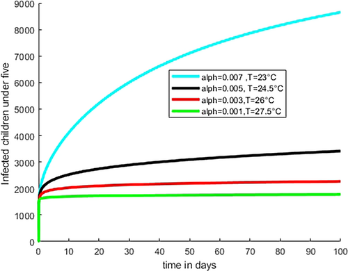
See Figures 2-5.

Details are in the caption following the image
Simulation of indicating the number of malaria occurrences in children under 5 years as increasing the alpha value with a decrease in temperature.
Details are in the caption following the image
The figure shows that the number of malaria cases in young individuals is decreasing with an increase in temperature.
Details are in the caption following the image
Simulation of indicating an increment of susceptible vector as an increase in fractional-order alpha and a decrease in temperature value.
Details are in the caption following the image
Simulation of indicating the increment of the infected vector as an increase in fractional-order alpha and a decrease in temperature value.

7.2 Numerical Simulation of Caputo Fractional-Order Model

The host population, which includes the human population and the vector population, is taken into account in the numerical simulation of the dynamics of malaria disease. The values of certain parameters are assumed to lie within the biologically feasible range, while the remaining parameters are adopted from published literature. The Adams–Bashforth numerical approach was used. The initial conditions described below and the parameter values listed in Tables 1 and 2 were used for simulations and analysis. The following initial requirements have been considered (Figures 6-17).

TABLE 1. Parameters Description 1.
Parameters Description Value Source
a j $$ {a}_j $$ Amplitude of function ψ ( T ) $$ \psi (T) $$ 0.011 Estimated
m $$ m $$ Maximum rate of eggs laid per oviposition 300 Estimated
a b $$ {a}_b $$ The amplitude of b ( T ) $$ b(T) $$ 0.015 [39, 49]
T e 2 $$ {T}_{e2} $$ Temperature at which P ( T ) $$ P(T) $$ is minimum 22°C Estimated
C a $$ {C}_a $$ The amplitude of P ( T ) $$ P(T) $$ 0.001 [39, 49]
d a $$ {d}_a $$ The minimum value of P ( T ) $$ P(T) $$ 0.15 [47]
s a $$ {s}_a $$ The maximum rate of transition between the aquatic stages 1.5 [47]
T e 1 $$ {T}_{e1} $$ The temperature at which ψ ( T ) $$ \psi (T) $$ is maximum 20°C Estimated
T b $$ {T}_b $$ The temperature at which b ( T ) $$ b(T) $$ is maximum 22°C [47]
TABLE 2. Parameters Description 2.
Parameters Description Value Source
π h $$ {\pi}_{\mathrm{h}} $$ Constant recruitment rate for humans 178 Assumption
μ h $$ {\boldsymbol{\mu}}_{\boldsymbol{h}} $$ The natural mortality rate of human 0.00004 [38]
ε c $$ {\boldsymbol{\varepsilon}}_{\boldsymbol{c}} $$ Number of bites on pre-school age people 0.479 [38]
ε y $$ {\boldsymbol{\varepsilon}}_{\boldsymbol{y}} $$ Number of bites on young age people 0.695 Assumption
b 1 ( T ) $$ {\boldsymbol{b}}_1(T) $$ Temperature-dependent fraction of bites that successfully infect human 0.456 Assumption
b 2 ( T ) $$ {\boldsymbol{b}}_2(T) $$ Temperature-dependent fraction of bites that successfully infect mosquitoes 0.574 Assumption
μ m ( T ) $$ {\boldsymbol{\mu}}_{\boldsymbol{m}}(T) $$ Temperature-dependent mortality mosquito 0.042 [38]
π m ( T ) $$ {\pi}_{\boldsymbol{m}}(T) $$ Recruitment for the mosquito population 50 Assumption
η $$ \boldsymbol{\eta} $$ Maturation rate of pre-school age people to 0.997 Assumption
φ 1 $$ {\varphi}_1 $$ Recovery rate by treatment of children under 5 age 0.0014 [38]
φ 2 $$ {\varphi}_2 $$ Recovery rate by treatment of young age 0.00000035 [38]
θ 1 $$ {\theta}_1 $$ The natural recovery rate of children under 5 age 0.6115 Assumption
θ 2 $$ {\theta}_2 $$ The natural recovery rate of young age 0.415 Assumption
f $$ \mathbf{f} $$ The transfer rate of humans from susceptible to the protected class 0.9988 Assumption
δ $$ \delta $$ The transfer rate of humans from the protected class to the susceptible class 0.62 Assumption
d 1 $$ {d}_1 $$ Disease-induced mortality rate for people under 5 (pre-school age) 2.14 × 10−6 [38]
d 2 $$ {d}_2 $$ The disease-induced mortality rate for people above five 9.78 × 10−8 [38]
γ $$ \boldsymbol{\gamma} $$ The proportion of new recruitments protected 0.99 Assumption
α 1 $$ {\alpha}_1 $$ The proportion of humans who lose their immunity and become susceptible 0.00042 Assumption
β $$ \beta $$ Rate of loss of immunity 0.222 Assumption
Details are in the caption following the image
The figure shows that for fractional order α = 1 , $$ \alpha =1, $$ the graph of the fractional-order model is similar to that of the graph of the integer-order model.
Details are in the caption following the image
The figure shows that susceptible human decrease as Caputo fractional order α $$ \upalpha $$ increases from α = 0.4 $$ \upalpha =0.4 $$ to α = 1 $$ \upalpha =1 $$ .
Details are in the caption following the image
The figure shows that as α $$ \upalpha $$ increases from α = 0.4 $$ \upalpha =0.4 $$ to α = 1 $$ \upalpha =1 $$ protective class individuals' increase.
Details are in the caption following the image
The figure shows that as fractional order increases from α = 0.4 $$ \upalpha =0.4 $$ to α = 1 $$ \upalpha =1 $$ infected children under 5 increases initially then decreases later.
Details are in the caption following the image
The figure shows infected young human increase as α $$ \upalpha $$ increases from α = 0.4 $$ \upalpha =0.4 $$ to α = 1 $$ \upalpha =1 $$ .
Details are in the caption following the image
The figure shows that recovered humans increase initially, and later decrease as Caputo fractional order α $$ \alpha $$ increases initially for α = 1 $$ \alpha =1 $$ and α = 0.95 $$ \alpha =0.95 $$ .
Details are in the caption following the image
The figure shows that as Caputo fractional order α $$ \upalpha $$ increases the susceptible vector decreases.
Details are in the caption following the image
The figure shows that infected vector increases initially, then after decreases as Caputo fractional order α $$ \upalpha $$ increases from α = 0.4 $$ \upalpha =0.4 $$ to α = 1 . $$ \upalpha =1. $$
Details are in the caption following the image
The figure shows that the number of infected under 5 human increases initially then decreases later as fractional order α $$ \upalpha $$ increases from α = 0.4 $$ \upalpha =0.4 $$ to α = 1 $$ \upalpha =1 $$ with biting rate b 1 $$ {b}_1 $$ increases from b 1 $$ {b}_1 $$ = 0.456 to 0.860.
Details are in the caption following the image
The figure illustrates that infected vector increases initially, then after decreases as fractional order α $$ \upalpha $$ increases from α = 0.4 $$ \upalpha =0.4 $$ to α = 1 $$ \upalpha =1 $$ with biting rate b 1 $$ {b}_1 $$ increases from b 1 $$ {b}_1 $$ = 0.456 to 0.860.
Details are in the caption following the image
The figure demonstrates that the cases in infected young human increase initially then later decrease as biting rate b 2 $$ {b}_2 $$ increases from b 2 $$ {b}_2 $$ = 0.574 to 0.978 with fractional order α $$ \upalpha $$ increases from α = 0.4 $$ \upalpha =0.4 $$ to α = 1 . $$ \upalpha =1. $$
Details are in the caption following the image
The figure illustrates that infected vector increases initially, then after decreases as fractional order α $$ \upalpha $$ increases from α = 0.4 $$ \upalpha =0.4 $$ to α = 1 $$ \upalpha =1 $$ with biting rate b 2 $$ {b}_2 $$ increases from b 2 $$ {b}_2 $$ = 0.574 to 0.978.
The initial requirements listed below have been taken into consideration:
S h ( 0 ) = 25891 , P h ( 0 ) = 8285 , I c ( 0 ) = 1542 , I y ( 0 ) = 1350 , R h ( 0 ) = 1543 , S m ( 0 ) = 11998 , I m ( 0 ) = 2601 . $$ {\displaystyle \begin{array}{cc}& {S}_h(0)=25891,{P}_h(0)=8285,{I}_c(0)=1542,{I}_y(0)=1350,\\ {}& {R}_h(0)=1543,{S}_m(0)=11998,{I}_m(0)=2601.\end{array}} $$

8 Result

Figure 2 illustrates how the fractional order rises from 0.001 to 0.007 with a difference of 0.002 as the temperature value drops from 27.5°C to 23°C with a difference of 1.5°C. This shows that temperature variability and fractional order have indirect relation to the transmission dynamics of disease that is as temperature increases beyond optimal temperature, the fractional order decreases. At extreme temperatures, the value of fractional order is low, and the rate of transmission is low because mosquitoes do not survive at such temperatures. As we observed from the figure at optimal temperature T = 23°C and at the highest listed fractional value α $$ \alpha $$ = 0.007, the number of infected children under 5 is high. Figure 3 shows that as the temperature rises from 23°C to 27.5°C, the fractional order α $$ \alpha $$ falls from 0.007 to 0.001; consequently, the number of infected young human decreases and at the optimal temperature T = 23°C and relatively high fractional order value α $$ \alpha $$ = 0, the number of infected young human increases.

Figures 4 and 5 demonstrate that an increase in susceptible and infected vectors, whose spikes correlated with an increase in the aquatic stage of mosquitoes and the number of mosquito–human contact rates or biting rates, was linked to a decrease in temperature from 27.5°C to 23°C and an increase in fractional order α $$ \alpha $$ from 0.001 to 0.007, respectively. On the other hand, the number of susceptible and infected vectors decreases as the temperature increases from 23°C to 27.5°C, and the fractional order falls from 0.007 to 0.001. This decrease in susceptible and infected vectors serves as an example of both the fall in human contact or biting rates due to an increase in adult-stage mosquito mortality and the decline in mosquito populations during the aquatic stage due to an increase in the aquatic stage death rate. As real-world biological facts indicate at high temperatures, the aquatic stage of mosquitoes and the adult stage of mosquitoes do not survive.

As illustrated in Figure 6, the Caputo fractional-order graph resembles a classical order graph where susceptible individuals first decline and subsequently rise. As the number of vulnerable people begins to decline, the number of people in the protected class rises as more people follow the recommendation given by responsible bodies to utilize protective gear, such as ITNs and IRS; as protective class individuals increase, then the number of infected population of both human and mosquito decreases. Figure 7 shows that similar to that of integer order, susceptible individuals decrease initially as Caputo fractional order α , $$ \alpha, $$ increases from α = 0.4 $$ \alpha =0.4 $$ to α = 1 $$ \alpha =1 $$ such decrement of susceptible individuals happened due to infection by infected mosquito, entering in protection class at the rate of f $$ f $$ and due to natural death rate then after start to increase due to recovered individuals and entrance of some individuals from protection class.

As shown in Figure 8, the population in the protective class increases when the number of vulnerable and recovered class members are urged to use malaria prevention tools, such as ITNs and IRS transfer from the susceptible and recovered groups to the protected class and, newly added individuals due to birth. Figure 9 illustrates that the number of infected children under 5 increases initially because of infection in the susceptible class as the Caputo fractional order α $$ \alpha $$ rises from α = 0.4 $$ \alpha =0.4 $$ to α = 1 . $$ \alpha =1. $$ As indicated in Figure 10, infected young human increase initially then decrease as fractional order α $$ \alpha $$ increases from α = 0.4 $$ \alpha =0.4 $$ to α = 1 . $$ \alpha =1. $$ At the same time number of susceptible young human decreases initially and the decrease as shown in Figure 7.

Figure 11 shows that recovered individuals increase initially for some fractional-order values, that is, for fractional order α $$ \alpha $$ = 1 and α $$ \alpha $$ = 0.95, then later decrease and the number of recovered individuals increases when the fractional-order values are far from integer order values as shown in the figure. As Figure 12 illustrates, the number of susceptible vector decreases as Caputo fractional order α $$ \alpha $$ increases from α = 0.4 $$ \alpha =0.4 $$ to α = 1 , $$ \alpha =1, $$ because at this range of α $$ \alpha $$ value, the number of infected individuals in both age level and number of infected vector are increased. As demonstrated in Figure 13, the number of infected vectors rises as Caputo fractional order α $$ \alpha $$ increases from α = 0.4 $$ \alpha =0.4 $$ to α = 1 . $$ \alpha =1. $$ Consequently, as indicated in Figures 9 and 10, the increment of number of cases in both age level is due to an increment in infected vector.

As the Caputo fractional order increases in Figures 9-11, we see that both infected humans decrease simultaneously, as illustrated in Figure 12. This indicates that when the infected human population declines, the recovered human population increases, as individuals from the infected compartment move into the recovered compartment as a result of the natural and clinical treatment recovery rate. Figures 9, 10, 12, and 13 show that as the susceptible vector compartment shrinks as a result of the infected human compartment, the number of susceptible vectors infected by biting both the infected people and the infected vector compartment increases.

Figure 14 indicates that the number of infected human under 5 increases initially and decreases later for biting rate of mosquitoes over under 5 human increases from b 1 = 0.456 $$ {b}_1=0.456 $$ to 0.860 as fractional order α $$ \alpha $$ increases from α = 0.4 $$ \alpha =0.4 $$ to α = 1 . $$ \alpha =1. $$ As indicated in Figure 15, the number of infected vectors increases initially then after decreases for biting rate b 1 $$ {b}_1 $$ over children under 5 human increases from b 1 = 0.456 $$ {b}_1=0.456 $$ to 0.860 as fractional order α $$ \alpha $$ increases from α = 0.4 $$ \alpha =0.4 $$ to α = 1 . $$ \alpha =1. $$

Figure 16 shows that the number of cases of young human increases initially then after decreases for biting rate of mosquito over young human increases from b1 = 0.456 to 0.86 as fractional order α $$ \alpha $$ increases from α = 0.4 $$ \alpha =0.4 $$ to α = 1 . $$ \alpha =1. $$ As demonstrated in Figure 17, the number of infected vectors increases initially then after decreases for biting rate b 2 $$ {b}_2 $$ over young human increases from b 2 = 0.574 $$ {b}_2=0.574 $$ to 0.978 as fractional order α $$ \alpha $$ increases from α = 0.4 $$ \alpha =0.4 $$ to α = 1 $$ \alpha =1 $$ .

As we observed in Figures 14-17, the biting rate of mosquitoes on children under 5 and young humans increases as the fractional order increases.

9 Conclusion

To better understand the dynamics of malaria across different age groups in human hosts, a fractional-order mathematical model was developed. This model, formulated as a system of differential equations, incorporated seven key state variables—five representing state variables of human population and two describing mosquito populations. Furthermore, the study explored the impact of temperature variations on malaria transmission, revealing critical insights into infection dynamics. The study highlighted the mathematical and epidemiological relevance of the fractional-order framework, demonstrating its applicability and significance. After a comprehensive investigation, we assessed the stability of both DFE and EE. By analyzing key model parameters that quantify the transmission severity of malaria, we determined the fundamental reproduction number, R 0 $$ {R}_0 $$ . This value serves as a critical indicator, predicting the average number of secondary infections (in both humans and mosquitoes) resulting from a single infectious individual during their infectious period. Our findings revealed that when R 0 < 1 $$ {R}_0<1 $$ , the system stabilizes at the DFE, indicating the disease will die out over time. Conversely, when R 0 > 1 $$ {R}_0>1 $$ , the system transitions to the EE, signifying the persistence of the disease within the population. Furthermore, we demonstrated how the Caputo fractional-order model was effectively simulated both with and without incorporating temperature variability.

The analysis reveals significant trends in the transmission dynamics of malaria. As the fractional order α $$ \alpha $$ increases, the number of cases across both age groups and the number of infected vectors also rise, as depicted in Figures 9, 10, and 13. Additionally, Figures 14-17 illustrate that the biting rate increases from b 1 = 0.456 $$ {b}_1=0.456 $$ to 0.860 $$ 0.860 $$ and b 2 = 0.574 $$ {b}_2=0.574 $$ to 0.978 $$ 0.978 $$ progressively as the fractional order α $$ \alpha $$ rises from α = 0.4 $$ \alpha =0.4 $$ to α = 1 $$ \alpha =1 $$ , which indicating a direct correlation between fractional order and mosquito biting rates across all age groups of infected humans. Furthermore, Figures 2-5 demonstrate that as temperature values increase, the fractional order decreases. This suggests an inverse relationship between fractional order and temperature variability, emphasizing how temperature fluctuations impact malaria transmission dynamics. These findings provide valuable insights into the interconnected factors influencing the spread of malaria.

Our study revealed critical biological insights into the relationship between temperature and malaria transmission. As temperatures rise beyond optimal levels, the biting rate of mosquitoes on infected humans significantly decreases. This reduction occurs because extreme temperatures are detrimental to mosquito survival. Moreover, these unfavorable conditions cause a decline in the fractional-order parameter, further reducing the number of malaria cases. The simulations were carried out using the Adams–Bashforth–Moulton numerical technique, providing valuable insights into the dynamics of malaria transmission under varying environmental conditions.

Plasmodium parasites are responsible for the spread of malaria. The following steps should be performed to eradicate or control malaria transmission dynamics because it is a global problem. The result of our study enforced encouraging and creating awareness in the use of several control techniques, like ITNs and IRS, in addition to various medical therapies, in order to prevent the dynamics of malaria disease transmission in the community. In addition to any other technique that lowers the rate of malaria infection, efforts should be made to use chemical or biological means to reduce mosquito populations and biting rates. Finally, in order to ensure the control or eradication of malaria transmission, public health decision-makers should prioritize intervention strategies to control malaria by targeting mosquito populations and reducing biting rates. Accordingly, responsible government bodies should implement and sustain effective programs that utilize control measures such as insecticide spraying, bed net distribution, treatment, and vaccination. These interventions, modeled as time-dependent variables, play a crucial role in minimizing human–mosquito contact and curbing the spread of malaria.

Caputo fractional-order derivatives are increasingly used to model infectious diseases because they account for the memory effect, that is, the disease dynamics depend not only on the current state but also on the history of infections, recoveries, or immunity. Accordingly, in our future research, we aim to expand our study to encompass the complete developmental aquatic stages of mosquitoes, integrating real-world climate variability data. Our focus will include the application of optimal control strategies incorporating different-order fractional derivatives with cost analysis, examining the effects of constant control measures on malaria prevalence. Furthermore, we will investigate the influence of rainfall, temperature, and humidity on malaria survival and mortality rates using fractional derivatives combined with optimal control approaches. To deepen our understanding, we plan to analyze malaria prevalence by calculating integer- and fractional-order derivatives, comparing the outcomes, and exploring key phenomena such as backward and forward bifurcation. We plan to apply Caputo fractional order on spatial dynamics of disease spread geographically in combination with fractional partial differential equations.

Author Contributions

Dawit Kechine Menbiko: investigation, writing – original draft, methodology, software, formal analysis. Chernet Tuge Deressa: supervision, resources, conceptualization.

Acknowledgments

The first author would like to thank the second author for his great support in the methodology and formal analysis of fractional models with and without temperature variability.

    Conflicts of Interest

    The authors declare no conflicts of interest.

    Data Availability Statement

    Data sharing is not applicable to this article as no new data were created or analyzed in this study.

      The full text of this article hosted at iucr.org is unavailable due to technical difficulties.