Deep Learning Based Visual Servo for Autonomous Aircraft Refueling
Funding: This work was supported by National Research Council of Thailand (NRCT), RDG6150074.
ABSTRACT
This study develops and evaluates a deep learning based visual servoing (DLBVS) control system for guiding industrial robots during aircraft refueling, aiming to enhance operational efficiency and precision. The system employs a monocular camera mounted on the robot's end effector to capture images of target objects—the refueling nozzle and bottom loading adapter—eliminating the need for prior calibration and simplifying real-world implementation. Using deep learning, the system identifies feature points on these objects to estimate their pose estimation, providing essential data for precise manipulation. The proposed method integrates two-stage neural networks with the Efficient Perspective-n-Point (EPnP) principle to determine the orientation and rotation angles, while an approximation principle based on feature point errors calculates linear positions. The DLBVS system effectively commands the robot arm to approach and interact with the targets, demonstrating reliable performance even under positional deviations. Quantitative results show translational errors below 0.5 mm and rotational errors under 1.5° for both the nozzle and adapter, showcasing the system's capability for intricate refueling operations. This work contributes a practical, calibration-free solution for enhancing automation in aerospace applications. The videos and data sets from the research are publicly accessible at https://tinyurl.com/CiRAxDLBVS.
1 Introduction
The integration of robots with sensors and deep learning techniques is a transformative development in automation [1]. It allows robots to handle complex tasks with adaptability, autonomy, precision, and efficiency, making them valuable assets in a wide range of industries, from manufacturing to health care and beyond [2]. This combination represents a significant step toward improving industrial robot capabilities and expanding their role in modern automation [3, 4]. The combination of human-eye-like cameras and deep learning approaches is a powerful solution for object inspection and classification in complex tasks like aircraft refueling. The technology can mimic human visual perception, enabling accurate and safe operations while also withstanding challenging environmental conditions. The combination of precision and durability makes it a valuable tool in the field of aviation and other industries where accurate object recognition and manipulation are essential.
Utilizing the precision and robustness previously discussed, robots have found practical applications in the realm of aircraft refueling. This adaptation serves the primary purpose of alleviating the physical strain on human operators who would otherwise be tasked with the laborious handling of bulky fuel lines. Additionally, it addresses the need for machinery capable of executing intricate and high-precision operations in this context. To meet these demands, an innovative approach has been adopted, known as the DLBVS technique. This technique functions as a control system that heavily relies on visual input derived from a camera. This camera captures real-time images of the operational environment, enabling the system to perform complex calculations related to the precise positioning and orientation of the intended target object [5, 6]. To enhance the robot's capabilities further, an advanced deep learning method has been employed, specifically leveraging the YOLOv4-tiny architecture [7-9]. Through this deep learning framework, the robot acquires the ability to recognize and understand distinctive features within its surroundings. This newfound knowledge greatly enhances its capacity to identify and interact with objects in a more sophisticated manner. In the execution of the robot's tasks, a camera is strategically affixed to its end effector, adopting an “eye-in-hand” configuration [10]. This camera plays a pivotal role by continuously capturing visual data, enabling the robot to calculate its speed and precisely monitor its own movements. This dynamic integration of camera data and target object information empowers the robot to navigate and manipulate itself with remarkable accuracy, effectively guiding it to the desired target pose estimation. The culmination of these cutting-edge technologies results in the development of a closed-loop control system. This system is particularly adept at minimizing discrepancies between the actual position of the robot and its intended position, significantly improving the overall operational precision. Consequently, it enhances the efficiency and safety of aircraft refueling processes, showcasing the transformative potential of these advancements in robotic technology.
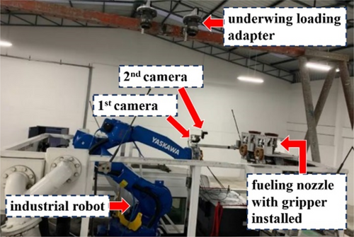
The gripper, which is a crucial component of the robot's end effector, is affixed in a specific configuration involving the use of two cameras, as depicted in Figure 1. To provide a more detailed explanation, the arrangement is as follows. One of the cameras (1st camera) is strategically positioned to focus on the underwing fueling nozzle. This camera is responsible for capturing visual data and images from this specific area of interest. It moves and adjusts its position as needed to maintain a clear and accurate view of the underwing fueling nozzle. The other camera (2nd camera) is dedicated to monitoring the bottom loading adapter, which is another essential part of the aircraft refueling process. Like the first camera, this second camera is designed to be movable, allowing it to track and maintain an optimal viewpoint of the bottom loading adapter.
This paper introduces a feedback closed-loop visual servo control system that excels in fault tolerance. It utilizes camera image acquisition and employs deep learning techniques to calculate camera velocity feedback, enhancing the robot's precision and adaptability. Furthermore, by utilizing the ROS framework for development [11-14], the paper emphasizes the efficiency and effectiveness of the control system's implementation. This approach offers great potential for advancing robotic control systems in various applications.
2 Related Work
2.1 Pose Estimation
The concept of pose estimation is a well-explored area in various fields, including spacecraft [15], satellites [16], autonomous underwater vehicles (AUVs) [17], fruit harvesting robots [18], unmanned aerial vehicles (UAVs) [19-21], and human [22] involving a multi-step process [23]. Pose estimation begins with object detection using Convolutional Neural Network (CNN), followed by the identification of 2D keypoints associated with 3D models. The PnP method is then used to establish the relationship between these keypoints and the 3D model, with CNN assisting in precise keypoint location determination. Additionally, neural style transfer is applied to generate various object textures, potentially improving the data set's richness and diversity. These techniques collectively contribute to accurate and robust pose estimation in these critical application domains [24]. The described CNN benefits from its efficiency and robustness in handling noisy data. To train and optimize the CNN effectively, a combination of real and synthetic images is used. Unreal Engine 4 is leveraged to create diverse and large data sets, and image augmentation techniques enhance the CNN's ability to handle different scenarios. These strategies collectively contribute to the development of a highly capable object detection system [15, 25]. The Yolo v3-tiny CNN architecture was employed to achieve precise 6 DOF pose estimation with a focus on accuracy while maintaining a relatively low number of parameters, considering the substantial parameter count associated with CNNs [26]. The enhanced YOLO-based pose estimation method involves a two-stage approach. The first stage predicts 2D keypoints on the object of interest, while the second stage leverages PnP to calculate the 6D pose estimation. This approach combines accuracy and speed in pose estimation. Additionally, augmentation techniques are applied to create a more robust and adaptable model that can handle various real-world conditions and object orientations [27-29].
2.2 Visual Servo Control System
The “eye-in-hand” method for calculating camera velocity using a pinhole camera model and the square root of the area is a technique commonly employed in visual servo control systems [30]. This approach simplifies the estimation of the pose estimation between the camera and an object in the world coordinate system. By combining Levenberg–Marquardt optimization with deep neural network-based relative pose estimation [31], along with data set optimization using image transfer techniques and the use of a Siamese network for 2-stage visual servo control, this approach aims to achieve high accuracy, robustness, and real-time performance in controlling the camera or robot's motion based on visual feedback. It leverages the power of machine learning and optimization to enhance the capabilities of the visual servo control system. Recent advancements highlight the synergy between deep learning techniques, such as DLBVS, for feature extraction and real-time processing in remote sensing applications. Notably, unmanned aerial vehicles (UAVs) and deep learning models such as YOLOv8 are transforming intelligent transportation systems (ITS) and smart city management by facilitating efficient monitoring and decision-making. UAVs, equipped with air quality sensors and cameras, enable dynamic data collection for traffic and pollution analysis [32, 33]. The integration of UAVs with YOLOv8 effectively addresses challenges, such as perspective distortions in aerial imagery, thereby improving detection accuracy [34]. Additionally, the lightweight YOLOv8-Nano model supports low-latency, resource-efficient detection on edge devices, enabling real-time ITS solutions in resource-constrained environments [35].
3 Working System
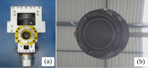
A system overview (Figure 1) depicts an illustration of the refueling aircraft system. This system is designed for the purpose of refueling aircraft, typically in an automated or robotic manner. The main components of the system include a robotic arm, a fuel nozzle, an adapter on the aircraft, and various sensors and cameras for guidance and control. The term “eye-in-hand cameras” typically refers to cameras that are mounted on the end effector of a robot, allowing them to observe the environment from the same perspective as the robot's end-effector. The first camera is oriented forward, facing the front of the robot and helps the robot locate and approach the fuel nozzle with precision, ensuring a secure connection. This is a crucial step in the refueling process as the robot needs to accurately pick up the nozzle to perform the refueling operation. The camera likely uses deep learning techniques to identify and track the position of the nozzle in its field of view as shown in Figure 2a. Once the nozzle is grasped, the upward-facing camera is used to align the nozzle with the adapter on the aircraft wing as shown in Figure 2b. These cameras play a critical role in the automation of the refueling process, ensuring accuracy and reliability in connecting the fuel nozzle to the aircraft's adapter, which is essential for the safe and efficient refueling of aircraft.
3.1 Diagram Nozzle Visual Servo Control System
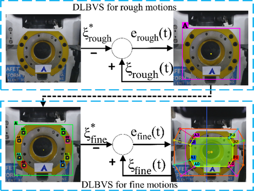
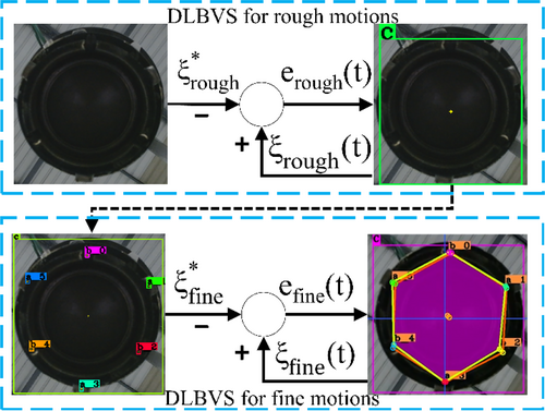
The system utilizes the first camera to capture images of the gripper image on the nozzle. It then uses a CNN-based visual servo closed-loop control method to process these images and make real-time decisions. The CNN likely extracts features from the gripper image and possibly other relevant visual cues. These features help the system understand the position and orientation of the gripper relative to the robot. Picking up the nozzle involves a sequence of movements, both rough and fine. The robot performs multiple motions to approach the nozzle accurately. These motions are carefully coordinated to ensure that the gripper aligns correctly with the nozzle. Initially, the system divides the motion trajectory into “rough motions.” These rough motions involve moving the robot in larger, less precise steps toward the target. Once the robot is close to the nozzle, it switches to “fine motions.” These fine motions are smaller and more precise movements, allowing the robot to achieve high accuracy in grasping the nozzle. These initial movements are designed to get the robot closer to the object without attempting to make a precise grasp yet. The system is designed to achieve a high level of accuracy in picking up the nozzle. This accuracy is crucial to ensure a secure connection for the refueling operation, as even minor misalignments could result in difficulties or safety issues during refueling. Figure 3 represents a visual depiction of the robot successfully picking up the nozzle with high precision. This visual feedback confirms that the robot's control system has successfully executed the planned trajectory and grasped the nozzle accurately. The result is a high-precision grasp, which is essential for the subsequent refueling process.
3.2 Diagram Adapter Visual Servo Control System
The adapter is described as having features like those of the nozzle. This suggests that, like the nozzle, the adapter may have distinctive visual markers or characteristics that the system can use for recognition and alignment purposes. The “lowest angle of rotation ωz” refers to a specific angular parameter. This parameter is likely used to describe the rotation of the adapter regarding its rotational characteristics and symmetry. The “ωz” value represents the angle of rotation around the z-axis which is described as a vertical axis running perpendicular to its front plane. This axis orientation is essential for understanding how the adapter can be rotated and aligned correctly. The adapter is noted to have three-fold rotational symmetry. This means that it can be rotated by 120° (360° divided by (3) around its center without changing its appearance. This symmetry is a crucial characteristic that simplifies the alignment process. The procedure involves having the fueling nozzle pushed firmly against the adapter. This step ensures that the nozzle and adapter are in close contact, ready for engagement. The next step is to rotate the nozzle slightly to the right or left. This rotation is likely along the z-axis, as mentioned earlier, and it can be in the range of 120° due to the adapter's three-fold rotational symmetry. As the nozzle is rotated, it will eventually reach a position where the locking mechanism on the nozzle aligns perfectly with the corresponding feature on the adapter. This mechanism is designed to secure the nozzle in place during the refueling process. The locking mechanism is described as typically being a latch or a hook. When the nozzle is rotated to the correct position and aligns precisely with the adapter's features, this latch or hook will click into place, indicating that the nozzle is securely locked onto the adapter. A visual depiction or diagram of the step-by-step workflow described above is shown in Figure 4.
4 Feature Extraction Using Neural Network
The process of extracting meaningful features from images can be challenging, especially when the observed object in the field of view lacks sufficient visual details. In some cases, the object of interest may not have distinctive characteristics that are easily recognizable. To address this challenge, additional image features are introduced during the feature extraction process. These additional features are likely to be visual cues or points of interest that can aid in the recognition and localization of the object. The image processing pipeline in this research employs a two-stage neural network for detecting specific image features. A two-stage network typically consists of two interconnected models, where the first stage performs a coarse task, and the second stage refines the results. This approach is often used to improve accuracy and efficiency. The YOLOv4-tiny model is employed in this stage to extract feature points labeled as A, A0, A1, A2, A3, B0, B1, B2, and B3 from the nozzle image. It was chosen for its balance of speed and efficiency, making it ideal for our hardware constraints. Its lightweight design ensures real-time performance on resource-limited devices, and its simplicity allowed seamless integration into the visual servoing pipeline. These labels likely represent distinct points or regions of interest within the nozzle image that are relevant to the subsequent robotic operation.
In the first stage of the neural network, the goal is to perform object detection to recognize a broader category of features labeled as “A” within a nozzle image. This “A” feature likely represents regions where the robot needs to insert its gripper. The network identifies and localizes this “A” feature within the image, providing information about its position and possibly its orientation.
After the first stage identifies the “A” feature, the second stage builds upon the first stage's results. It uses the YOLOv4-tiny model specifically to detect and extract the more detailed feature points labeled A0, A1, A2, A3, B0, B1, B2, and B3, helping to eliminate false positives or unwanted detections. This stage aims to refine the initial detection results and detect additional features. The network in the second stage is likely configured for multi-class detection, with each class corresponding to one of the labeled features. It identifies and classifies these features based on their visual characteristics.
By employing the two-stage learning technique, the system can effectively reduce surrounding noise in the image. Surrounding noise may include irrelevant objects or visual elements that could interfere with accurate feature detection.
Figure 5 represents a visual representation of the complete detection result achieved through this two-stage learning technique. It showcases the identified feature points A0, A1, A2, A3, B0, B1, B2, and B3 within the nozzle image. This approach improves the identification of specific feature points within the nozzle image, reducing surrounding noise and providing precise information that can guide the robot's actions during tasks such as gripper insertion or alignment.
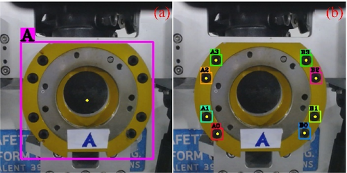
In addition, a trained model for the first stage can identify and isolate regions of interest within images by detecting these feature points or landmarks within an image that have been identified as being significant for the task at hand. Feature points can be used for various purposes, such as aligning images or detecting key elements within an image. Figure 6 visually illustrates the process described above. It shows examples of bounding boxes, cropped areas, and feature points in the context of the model's operation.
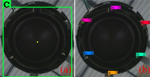
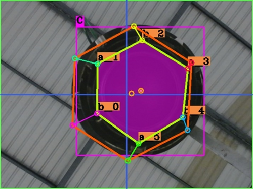
Similarly, an adapter image data set was also trained like the nozzle image; however, in the second stage, training six feature points are divided into 3 tabs (a_1, a_3, and a_5) which are small, protruding pieces of metal located on the aircraft's adapter, and 3 notches (b_0, b_2, and b_4) which are small, rectangular or square-shaped cutouts located on the end of the adapter shown in Figure 7b and the result of two-stage adapter detection including 6 feature points is shown in Figure 8.
5 Design a Data Set for Training
The design of the training data set is a critical and intricate step in training deep learning models. It impacts not only the precision and robustness of the model's results but also its ability to generalize to new situations. The training data set must be designed to facilitate this generalization. In our research, it contains enough representative examples to capture the underlying patterns or features in the data without overfitting. A well-designed data set, divided into two stages and augmented with various techniques, is essential for the success of a deep learning approach. It ensures that the model is accurate, robust, and capable of generalizing to different environments and conditions, ultimately leading to more precise results in real-world applications. Figure 9 provides a visual representation of some divided data sets and the data augmentation techniques used. It helps convey how the data set is structured and augmented for the deep learning process. The illustration may show examples of images before and after augmentation to highlight the variations.
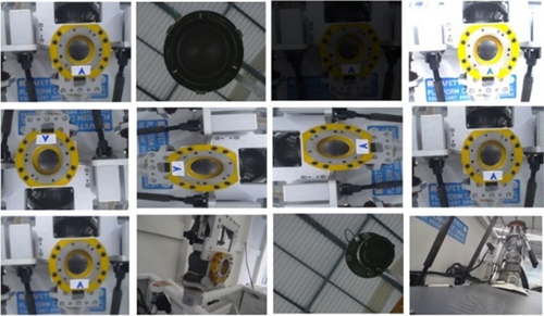
The use of randomization in the second stage data set is a key strategy to ensure that the deep learning model is versatile, robust, and capable of handling diverse real-world conditions. It helps the model generalize its knowledge and avoid overfitting while mimicking the variability encountered in practical applications. Figure 10 shows a visual representation of some randomization images to provide a clear understanding of how it contributes to data set diversity and model performance. The use of a data set with only one nozzle and adapter image limits a comprehensive evaluation of the model's performance. Future work will expand the data set to include a wider range of nozzles, adapters, and real-world images, enhancing the model's evaluation, robustness, and reliability in practical applications.

The positional values obtained from the bounding boxes in the initial deep learning stage were utilized to crop and acquire images for the purpose of auto-data labeling. In this research, we initially gathered 261 images for training in both the first and second stages. After implementing data augmentation techniques, the quantity of images for each stage surged to 10,440, showcasing a remarkable diversity in various environmental contexts.
Subsequently, our models underwent training, utilizing an Nvidia GTX 1080 TI graphics card, for a duration of 6 h. During this training period, the accuracy reached approximately 99.0%, while the average loss was maintained at around 0.05%. Table 1 presents the hyperparameters employed in our models.
| Parameter | CNN model |
|---|---|
| Input image size | 416 × 416 pixels |
| Batch size | 64 |
| Learning rate | 0.001 |
| Maximum Epoch | 500 |
| Loss function | Cross-entropy |
| Optimizer | Stochastic Gradient Descent |
6 Uncalibrated Monocular Camera Visual Servo Control System
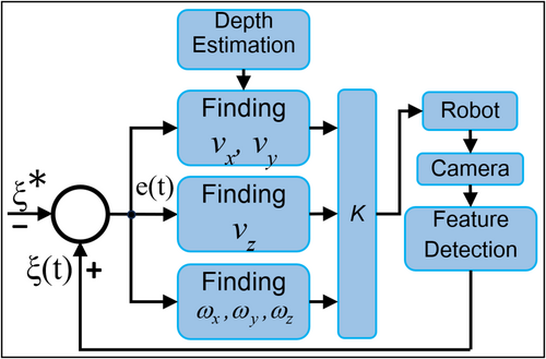
We employed a monocular camera to capture an eye-in-hand image as the input for our system, and we implemented a two-stage visual servo control system. This allowed us to extract the feature point vector S, illustrated in Figure 5 and Figure 7, comprising points A0, A1, A2, A3, B0, B1, B2, and B3 for a nozzle, as well as points b_0, a_1, b_2, a_3, b_4, and a_5 for an adapter. Subsequently, we automated the construction of polygons for both the nozzle and the adapter by connecting these feature points. This process enabled us to identify the centroids and calculate the areas of these polygons. To assess the control loop's performance, we determined the error, denoted as e(t), by comparing the actual feature vector with the desired feature vector ξ*. Subsequently, we decomposed the camera velocity into translational velocities and rotational velocities ().
Specifically, we can compute , , and by employing EPnP method, while (including ) is determined through the centroid polygon error. The estimation of relies on depth estimation, which is derived from the error associated with the polygon region. To regulate the robot's movement, we applied proportional control by multiplying the gain matrix K with the camera velocity value, resulting in a signal u(t) for robot control. Throughout the robot's motion to a new pose estimation, we repeatedly acquired the camera image for calculations within the control loop, as depicted in Figure 11. This process continued until the error signal fell below the predefined threshold.
6.1 The Procedure for Determining the Angular Velocity
- The process begins by extracting the pixel positions of feature points. These feature points are obtained through a neural network, with each feature point having an associated object point (representing the desired position) and an image point (representing the actual position).
- Once having the pixel positions of both the object point (desired position) and the image point (actual position), we proceed to determine the angular velocity using the EPnP method.
-
Setting the camera intrinsic matrix to
where is determined as the maximum value between the width () and height () of the image. This value is crucial for scaling the intrinsic matrix.
6.2 The Procedure for Determining the Translational Velocities Along the x-Axis and y-Axis
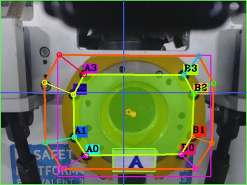
Here's what each variable in these equations represents: and the centroid points of the polygon at the actual (current) position. and are the centroid points of the polygon at the desired position (as shown in Figure 6 and Figure 8). and are scalar gain coefficients. These coefficients are determined by comparing the positions of the robot at both the actual and desired positions. Specifically, they represent a ratio of linear displacement from the object along the z-axis (depth) between these two positions.
6.3 The Procedure for Determining the Translational Velocity Along the z-Axis
6.4 Proportional Control
7 Experimental Results
This experiment involves using a webcam attached to a Yaskawa GP25 robot to capture images. The DLBVS technique is applied to guide the robot to specific target pose estimations related to a nozzle and an adapter. The control system operates within the ROS framework, receiving camera velocity commands via a TCP/IP connection to drive the robot's movements. This setup allows for precise control and alignment of the robot with respect to the specified goal points on the objects. Figure 12 depicts the locations of the desired feature points as well as the various pose estimations associated with the nozzle. These pose estimations, including the initial and steady-state pose estimations, are essential for guiding the robotic system to perform specific tasks, such as plugging a gripper into the nozzle, with precision and accuracy.
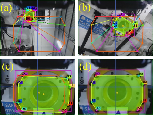
Figure 12a showcases the initial pose estimation of the nozzle. This initial position and orientation of the nozzle serve as the starting point for the robotic operation or manipulation task. The depicted pose estimation is essential as it provides a reference point from which the robot can execute its movements and tasks.
In Figure 12b, the system has started to adjust the pose estimation of the nozzle to move it closer to the desired pose estimation. We can observe the nozzle transitioning or beginning to align with the target position and orientation. In Figure 12c, the nozzle is getting closer to the desired pose estimation. The discrepancy between the yellow and orange octagon outlines is decreasing, indicating that the control system is successfully guiding the nozzle toward the target pose estimation. It may not yet be perfectly aligned but is approaching the desired orientation and position. Finally, when the nozzle has reached the desired pose estimation, the yellow octagon outline aligns perfectly with the orange one. This stage represents the successful completion of the control task, as shown in Figure 12d.
Figure 13a displays the initial pose estimation of the adapter. This initial configuration serves as the starting point for the robotic operation or manipulation task involving the adapter. Understanding the initial pose estimation is essential, as it provides a reference for the robot to plan and execute its movements.
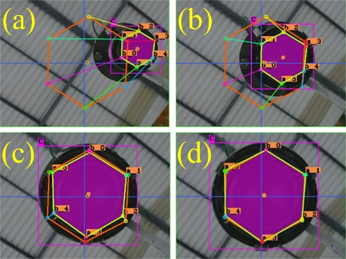
In Figure 13b, the desired pose estimation of the adapter can be clearly observed. This represents the specific pose estimation that the robotic system aims to achieve concerning the adapter. The area of the polygon outlined in the figure is derived from feature points labeled as b_0, a_1, b_2, a_3, b_4, and a_5. These feature points play a crucial role in defining the adapter's geometry and alignment. In Figure 13c, the system is steadily converging toward the desired pose estimation, as evidenced by the gradual reduction of the distance between the yellow hexagon and the orange one. This demonstrates the successful guidance provided by the control system in steering the system toward its intended target pose estimation. Figure 13d shows the culmination of the control system's efforts in positioning the adapter precisely for attaching the adaptor. This alignment is critical for ensuring the success of the overall task or operation, emphasizing the importance of precision and accuracy.
This robotic process involves two primary steps. Initially, the robot utilizes DLBVS to identify and secure a nozzle in the desired initial positions. Employing advanced deep learning techniques, it detects and precisely locates the nozzle within captured images. Subsequently, it extracts distinctive feature points denoted as A0, A1, A2, A3, B3, B2, B1, and B0 from these images to monitor the nozzle's position. The system then computes the error between the desired and current nozzle orientations, as determined by a camera. This disparity serves as a reference for a feedback control system, which in turn directs the robot's motions to align perfectly with the nozzle. Once the desired alignment is achieved, the robot's manipulator seizes the nozzle for subsequent tasks. Following the nozzle pickup, the robot advances to the process of affixing it to an adapter. DLBVS is again employed to locate the adapter in the desired initial configurations. Feature points, specifically denoted as b_0, a_1, b_2, a_3, b_4, and a_5, are extracted to meticulously track the adapter's precise position. The system then computes the error between the desired and current adapter orientations, utilizing input from an additional camera. This disparity generates a feedback control signal that navigates the robot's movements, ensuring precise alignment with the adapter. Upon reaching the desired pose estimation, the robot activates its gripper mechanism to transport the nozzle toward the adapter, where it is securely inserted and locked at the inlet end.
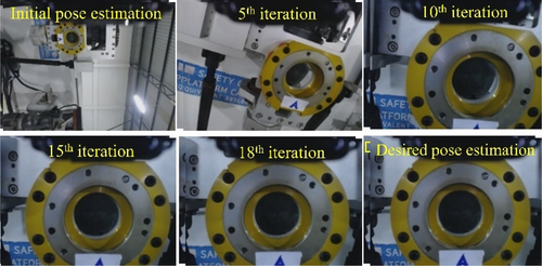
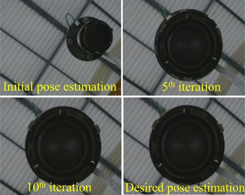
The initial pose estimation exhibits inconsistencies in illumination and a notable difference in z-axis rotation, as depicted in Figure 14. Nonetheless, through the implementation of DLBVS and data set augmentation, noise is effectively minimized, and the resilience of feature points is heightened. The original images of the adapter's posture are captured in a dimly lit and dark environment, as demonstrated in Figure 15. Remarkably, even when the feature points are scarcely discernible due to the challenging lighting conditions, the DLBVS remains capable of locating them. It's noteworthy that there were no deliberate efforts to attain ideal lighting conditions, and no external alterations in lighting or obstructions were introduced during the process.
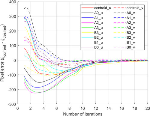
The discrepancies in pixels between the desired nozzle pose estimation and its current position and orientation, which guide the robot to attain the desired pose estimation, are visualized in Figure 16 for both the horizontal (u) and vertical (v) axes within the camera image plane. As the robot progressively approaches the target pose estimation, this graph depicts a consistent reduction in pixel errors with each iteration. Nevertheless, it's important to note that pixel errors may exhibit minor fluctuations owing to factors like alterations in lighting, obstructions, or other environmental variables. Notably, our DLBVS approach showcases convergence devoid of erratic or oscillatory behavior as the number of iterations increases. As the robot advances closer to the desired pose estimation, the pixel errors consistently decrease. This graph serves as an indicator of the system's convergence rate and provides insights into any potential issues requiring attention and resolution. In Figure 17, we depict the translational deviations along the x, y, and z axes, highlighting the disparities between the current position of the nozzle and its desired location. As the robot progressively approaches the intended position, these translational errors diminish incrementally with each iteration, eventually stabilizing at a consistent level. This stabilization marks the moment when the robot successfully attains the target position. The figure effectively conveys the system's rate of approach toward the desired position, offering a clear indication of its progress and the absence of any significant issues in the process.
Concerning rotational errors, these errors diminish progressively as the robot approaches the desired orientation. The graphical representation in Figure 18 serves as a visual indicator of the system's rate of approach toward the intended orientation. Ideally, this graph exhibits a consistent and gradual reduction in rotational errors as time progresses, ultimately reaching a stable state. This stabilization signifies that the robot has successfully attained the desired orientation. In essence, Figure 18 provides valuable insights into how swiftly and effectively the system aligns itself with the desired orientation. A smooth and continuous reduction in errors suggests that the robot's control system is operating optimally, ensuring precise alignment without any notable issues.
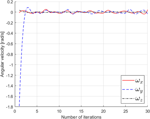
Figures 19, 20 illustrate the robot's translational and angular velocities as it approaches the nozzle, providing valuable insights into the robot's motion characteristics. Initially, during the first six iterations, these velocities gradually approach zero. This initial phase involves the robot initiating its movement, encompassing adjustments in rotation around the x, y, and z axes, as well as translational velocities (vx and vy) within the xy plane. Subsequently, a notable reduction in translational velocity along the z-axis (vz) occurs in each servo cycle as the robot approaches its target. This decline in vz is significant because it facilitates a swift convergence of the system, enabling it to efficiently achieve the desired image features related to the nozzle.
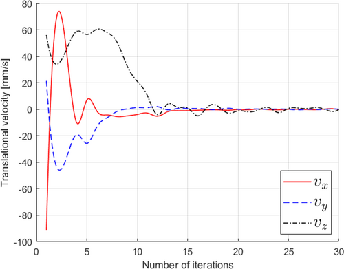
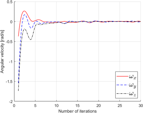
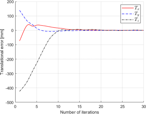
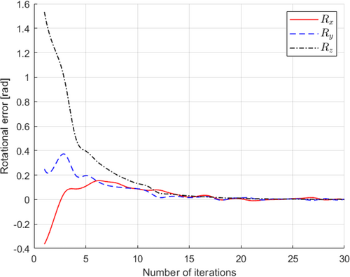
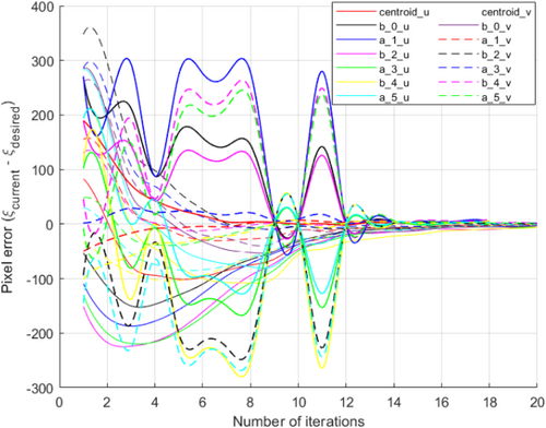
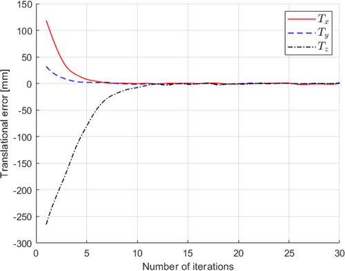
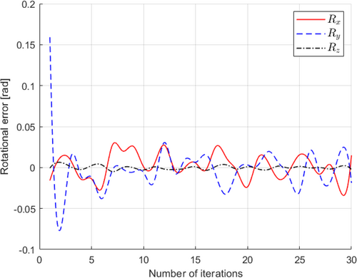
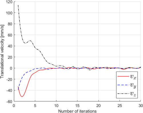
Likewise, in Figure 21, we observe the pixel errors associated with selected feature points as they relate to the desired and current pose estimation of the adapter. These errors are tracked along the horizontal (u) and vertical (v) axes within the camera's image plane. Notably, pixel errors exhibit some fluctuations during the DLBVS process, primarily due to the inherent challenges in visual feature extraction. However, the overarching trend is towards error reduction. As the robot steadily progresses through iterations, there is a consistent and gradual decline in pixel errors for all feature points. This decline culminates at the 18th iteration, marking the robot's successful approach to the target pose estimation. Additionally, Figure 22 presents translational errors along the x, y, and z axes, characterizing the disparities between the adapter's current and desired positions. As the robot advances toward the target position, these translational errors decrease with each iteration, eventually stabilizing to signify that the robot has precisely reached its intended location. Figure 23 showcases rotational errors, which exhibit slight oscillations over time due to the visual feature extraction process, particularly concerning small rotation angle offsets. Despite these observable oscillations, the robot maintains a secure connection between its gripper and the adapter. This signifies that these errors remain within a range of ± 1.5°, and the robot effectively achieves the desired orientation. In addition, Figures 24 and 25 portray the translational and angular velocities of the robot during its movement toward the adapter. Notably, all of these velocities converge to nearly zero by the 15th iteration, indicating a gradual deceleration of the robot's motion as it approaches the target, ensuring precise and controlled positioning.
8 Conclusion
Effective depth estimation and EPnP methods have been successfully integrated into a DLBVS feedback control system employed in a robotics application for demonstrating aircraft refueling. This system enables precise control of robot movements using visual data from a non-calibrated monocular camera. This approach offers several notable advantages compared to alternative visual servoing methods. It exhibits robustness when faced with variations in lighting conditions and changes in the appearance of the target object. Moreover, it excels in handling target objects with intricate shapes, such as the octagonal nozzle and hexagonal adapter involved in this context. The implementation of a two-stage deep learning technique plays a pivotal role in locating specific feature points on the target objects and enhancing the overall resilience of the control system. It empowers the system to extract valuable insights from images of the nozzle and adapter, further simplifying and resolving complexities. The overall complexity of the system is substantially reduced and effectively addressed. Consequently, the feedback control system, in tandem with camera velocity estimation, adeptly guides the robot to the desired pose estimation. The outcome of this integration is highly accurate, with translational errors of less than 0.5 mm for both the nozzle and adapter. Additionally, rotational errors remain under 1.5° for both components when positioned in the desired pose estimation. This demonstrates the system's precision and efficiency in achieving the intended outcomes.
Author Contributions
Natthaphop Phatthamolrat: conceptualization, data curation, software, visualization, methodology, investigation, writing – original draft, validation, project administration. Teerawat Tongloy: resources, software, data curation, validation. Siridech Boonsang: writing – review and editing, methodology, resources, supervision. Santhad Chuwongin: writing – original draft, writing – review and editing, funding acquisition, supervision, conceptualization, methodology, visualization, investigation.
Acknowledgments
This work was financially supported by the National Research Council of Thailand (NRCT) [RDG6150074], which has provided financial support for the research project. We are grateful to BAFS Innovation Development Co. Ltd. for providing some facilities for this project.
Conflicts of Interest
The authors declare no conflicts of interest.
Open Research
Data Availability Statement
The data that support the findings of this study are available on request from the corresponding author. The data are not publicly available due to privacy or ethical restrictions.


