Improved Conjugate Gradient Methods for Unconstrained Minimization Problems and Training Recurrent Neural Network
ABSTRACT
This research introduces two conjugate gradient methods, BIV1 and BIV2, designed to enhance the efficiency and performance of unconstrained optimization problems with only first derivative vectors. The study explores the derivation of new conjugate gradient parameters and investigates their practical performance. The proposed BIV1 and BIV2 methods are compared with the traditional Hestenes-Stiefel (HS) method through a series of numerical experiments. These experiments evaluate the methods on various test problems sourced from the CUTE library and other unconstrained problem collections. Key performance metrics, including the number of iterations, function evaluations, and CPU time, demonstrate that both BIV1 and BIV2 methods offer superior efficiency and effectiveness compared to the HS method. Furthermore, the effectiveness of these methods is illustrated in the context of training artificial neural networks. Experimental results show that the new methods achieve competitive performance in terms of convergence rate and accuracy.
1 Introduction
The CG method has garnered significant attention in recent years due to its wide applicability in solving unconstrained optimization problems. Its favorable properties, such as global convergence and low memory requirements, have made it a key tool in many fields. Many of the advanced CG methods proposed in the literature are modifications or enhancements of the classical CG methods, aiming to improve their efficiency and robustness in practical applications [11-13]. The scope of CG methods has expanded to encompass applications in diverse areas such as data estimation [14], image restoration [15-18], and signal processing [19, 20].
In recent years, with the increasing demand for AI in various fields, CG methods have become an essential tool in training artificial neural networks. The gradient-based optimization techniques employed in these networks are crucial for achieving accurate and efficient learning ([12, 21-23]).
Recent studies have further advanced the CG method in the context of machine learning. For instance, a stochastic three-term conjugate gradient method with variance reduction for non-convex learning was proposed by [24]. This method aims to improve the efficiency of stochastic gradient descent in machine learning applications, where the slow convergence of traditional methods can be a limitation. By integrating variance reduction techniques with the CG method, the authors achieved linear convergence under less stringent assumptions, thereby enhancing both theoretical and practical performance for non-convex machine learning models.
Similarly, Huang [25] introduced a biased stochastic conjugate gradient algorithm with an adaptive step size for non-convex problems. This algorithm combines the stochastic recursive gradient method with the Barzilai–Borwein (BB) technique to improve step size selection, avoiding issues associated with fixed step sizes. The BSCG algorithm has demonstrated strong competitiveness, offering global optimal convergence and linear convergence rates for non-convex functions, with promising numerical results across machine learning applications.
Beyond machine learning, optimization techniques have been applied to various engineering fields. For example, studies by [26] utilized advanced metaheuristic algorithms, such as Depth Information-Based Differential Evolution (Di-DE), to enhance the precision of Proton Exchange Membrane Fuel Cell (PEMFC) parameter estimation. Their algorithm demonstrated excellent performance in optimizing parameters for multiple PEMFC models, offering substantial improvements in both runtime and accuracy compared to conventional methods. This work underscores the significance of optimization techniques in enhancing the design and operation of clean energy systems.
Additionally, the integration of machine learning and finite element methods has proven effective in investigating the axial compressive behavior of elliptical FRP-confined concrete columns. Yue [27] utilized machine learning models, such as XGBoost, to predict the compressive strength of concrete columns, achieving high predictive accuracy. Their work highlights the power of combining computational methods with machine learning to optimize engineering analysis.
Optimization techniques have also found applications in environmental research. For instance, [28] proposed a novel approach for analyzing marine life in the polar regions using advanced machine learning techniques. Their model achieved impressive accuracy and precision, underscoring the potential of combining environmental monitoring with machine learning to ensure sustainable food security in fragile ecosystems.
These studies collectively demonstrate the transformative role of optimization methods and machine learning in solving complex, real-world problems across a wide range of domains. From machine learning and energy systems to environmental analysis, the continued development of these techniques promises to drive innovation and improve efficiency in various industries.
The increasing demand for advanced optimization methods in machine learning and engineering has highlighted the limitations of classical techniques, such as the HS and FR methods. These methods often face challenges like slow convergence and inefficiency in handling large-scale problems. To address these limitations, this paper introduces two novel conjugate gradient methods, BIV1 and BIV2, that enhance convergence speed and robustness while maintaining computational efficiency. These methods are validated through extensive numerical experiments and real-world applications, demonstrating their potential in training artificial neural networks and solving complex optimization problems with higher precision.
The structure of this paper is as follows: Section 2 presents the proposed method in detail. Section 3 establishes the global convergence properties of the method. Finally, Section 4 provides numerical results to illustrate the performance and practical benefits of the method.
2 The Derivation of the Algorithm
The terms in (5a) and (5b), illustrate how the conjugate gradient method adjusts its search direction based on the gradient differences, the function values, and additional properties of the objective function.
The newly developed conjugate gradient methods, termed BIV1 and BIV2, aim to improve the efficiency and convergence characteristics of traditional conjugate gradient approaches, particularly in high-dimensional optimization scenarios. The algorithm outline is presented next (Algorithm 1).
ALGORITHM 1.
- Step 1:
(Initialization) Given an initial point , parameters, and . Set , and .
- Step 2:
If then stop.
- Step 3:
Compute the step size by the weak Wolfe line search [29, 30],
- Step 4:
Generate the next iteration by (2).
- Step 5:
Compute by (3) and choose an appropriate conjugate parameter by (11) or (12).
- Step 6:
Set and go to Step 1.
3 Algorithm Convergence Characteristics
This section outlines the key properties of the new algorithm, including its descent property, and global convergence. The following necessary assumptions about the objective function are considered as essential for the analysis to follow.
Assumption 1.
- Bounded Level Set: The level set at is bounded. There exists a constant such that:
(13)
- Lipschitz Continuity of the Gradient: In some neighborhood of , the function is continuously differentiable, and its gradient is Lipschitz continuous with Lipschitz constant , This implies:
(14)
- Bounded Gradient: There exists a positive constant such that:
(15)
- Strong Convexity: If is strongly convex, then there exists a constant , such that:
(16)
These assumptions are fundamental for establishing the global convergence of optimization algorithms, ensuring that the level sets are manageable, the gradient does not oscillate excessively, and the function exhibits desirable convexity properties.
We start with the analysis of the descent property of the methods to ensure a reduction in the objective function value. This property is fundamental for the convergence of optimization methods, ensuring that the algorithm consistently moves toward a minimum.
Theorem 1.Suppose that assumption (1) holds, then the sequence of search directions yielded by BIV1 and BIV2 satisfies:
Therefore if , the search direction satisfies . A BIV1 method's similar descending feature is demonstrated.
Now, the global convergence of the algorithm is established by demonstrating that, under appropriate conditions, the sequence generated by the algorithm converges to a stationary point of the objective function. This characteristic is vital for ensuring the reliability of the algorithm in solving a wide range of unconstrained optimization problems.
It may be inferred that Dai et al. [31] established the necessary condition for CG techniques to converge while using Wolfe line search conditions mentioned in Step 3 of the algorithm outline.
Theorem 2.Suppose that assumption (1) holds and the sequences and are generated by BIV1 and BIV2 Algorithms. Also, let be strongly convex then:
Therefore, we get . Also, the same can be similarly shown for BIV2 method.
4 Numerical Results
This section presents the numerical results to assess the performance of the proposed BIV1 and BIV2 methods for solving unconstrained optimization problems and training neural networks.
4.1 Unconstrained Optimization Problems
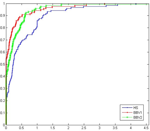
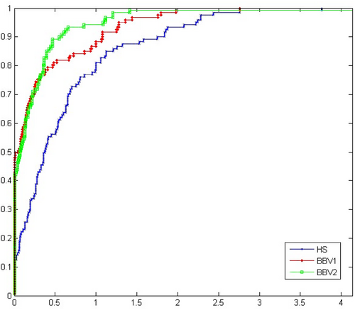
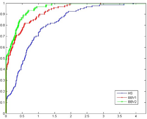
In this subsection, a series of experiments is conducted to evaluate the effectiveness of the BIV1 and BIV2 methods. The performance of these methods is compared with that of the original HS method [27]. The test problems are sourced from the CUTE library [32], in addition to other unconstrained problem collections [33, 34]. The problems vary in dimensionality. To ensure a fair comparison, all methods utilize the weak Wolfe line search for computing the step length , with the parameters set to in Step 3 of the algorithmic outline. Instances where a method fails to converge are denoted by “F”. The implementations are coded in MATLAB 2013b and executed on an HP i5 CPU. The results are summarized in Table 2, which includes the number of iterations (NOI), number of function evaluations (NOF), and CPU time (CPUT) for each method. Additionally, performance profiles proposed by Dolan and Moré e [35] are used to visually represent the performance of the algorithms in terms of CPUT, NOI, and NOF. In these profiles, the top curve indicates the superior performance of the corresponding method. For a detailed interpretation of the performance profiles (see [35]). Figures 1-3 graphically demonstrate the effectiveness of the proposed methods.
| HS | BIV1 | BIV2 | ||||||||
|---|---|---|---|---|---|---|---|---|---|---|
| Test function | Dimension | NOI | NOF | CPUT | NOI | NOF | CPUT | NOI | NOF | CPUT |
| dixmaana | 1500 | 29 | 110 | 0.316537 | 18 | 71 | 0.180405 | 28 | 98 | 0.259175 |
| 3000 | 29 | 111 | 0.706153 | 24 | 85 | 0.543393 | 33 | 106 | 0.68775 | |
| 15,000 | 30 | 102 | 2.23231 | 25 | 106 | 1.968824 | 31 | 96 | 1.79831 | |
| 30,000 | 30 | 108 | 7.998396 | 23 | 112 | 3.737099 | 24 | 89 | 2.492262 | |
| dixmaanb | 1500 | 24 | 109 | 0.201828 | 25 | 95 | 0.134428 | 25 | 91 | 0.135213 |
| 3000 | 21 | 120 | 0.343729 | 28 | 99 | 0.361824 | 32 | 135 | 0.449273 | |
| 15,000 | 32 | 150 | 2.061474 | 31 | 134 | 1.849407 | 29 | 113 | 1.494153 | |
| 30,000 | 29 | 158 | 4.226191 | 58 | 202 | 5.354701 | 25 | 105 | 2.796302 | |
| dixmaanc | 1500 | 29 | 119 | 0.203829 | 25 | 101 | 0.146666 | 25 | 114 | 0.148214 |
| 3000 | 31 | 170 | 0.55656 | 29 | 114 | 0.36507 | 27 | 108 | 0.359118 | |
| 3500 | 31 | 170 | 0.569967 | 29 | 114 | 0.408739 | 27 | 108 | 0.340748 | |
| dixmaanh | 150 | 73 | 159 | 0.074138 | 84 | 289 | 0.060672 | 100 | 162 | 0.043974 |
| 300 | 110 | 211 | 0.075646 | 123 | 369 | 0.115186 | 118 | 176 | 0.068489 | |
| 1500 | 220 | 359 | 0.489699 | 399 | 991 | 1.249954 | 184 | 252 | 0.318739 | |
| 3000 | 279 | 450 | 1.47394 | 450 | 1186 | 3.742389 | 263 | 342 | 1.068857 | |
| dixmaani | 150 | 914 | 1324 | 0.317954 | 509 | 1524 | 0.350794 | 699 | 761 | 0.174667 |
| 300 | 1835 | 2688 | 0.912329 | 1690 | 4365 | 1.488733 | 1610 | 1701 | 0.594278 | |
| dixmaank | 30,000 | 523 | 770 | 30.0027 | 263 | 720 | 28.09845 | 560 | 649 | 25.53606 |
| dixmaanl | 1500 | 361 | 542 | 1.081864 | 270 | 825 | 1.623452 | 274 | 344 | 0.713821 |
| 3000 | 324 | 503 | 2.067315 | 243 | 702 | 3.027228 | 833 | 906 | 3.862978 | |
| dixon3dq | 4 | 36 | 84 | 0.012875 | 34 | 80 | 0.00452 | 42 | 92 | 0.005674 |
| 10 | 95 | 173 | 0.011285 | 67 | 112 | 0.009195 | 79 | 139 | 0.009589 | |
| 50 | 500 | 742 | 0.052055 | 488 | 722 | 0.048882 | 431 | 580 | 0.036346 | |
| 150 | F | F | F | 1543 | 2200 | 0.152255 | 1791 | 2396 | 0.184449 | |
| dqdrtic | 500 | 63 | 215 | 0.039847 | 62 | 215 | 0.014765 | 58 | 189 | 0.012824 |
| 1000 | 57 | 200 | 0.022139 | 57 | 212 | 0.023357 | 85 | 309 | 0.034885 | |
| 5000 | 87 | 225 | 0.112033 | 81 | 253 | 0.127161 | 83 | 287 | 0.146353 | |
| 10,000 | 80 | 276 | 0.245279 | 85 | 254 | 0.242468 | 68 | 228 | 0.218394 | |
| edensch | 500 | 41 | 120 | 0.052105 | 47 | 135 | 0.049649 | 43 | 115 | 0.041321 |
| 1000 | 38 | 129 | 0.076774 | 37 | 104 | 0.057072 | 45 | 115 | 0.062021 | |
| 5000 | 59 | 209 | 0.628168 | 43 | 155 | 0.470628 | 33 | 108 | 0.330272 | |
| 10,000 | 66 | 366 | 2.209617 | 42 | 127 | 0.752922 | 63 | 338 | 1.995954 | |
| eg2 | 4 | 62 | 269 | 0.0258 | 53 | 149 | 0.011001 | 28 | 90 | 0.005776 |
| 10 | 170 | 527 | 0.02691 | 40 | 113 | 0.00783 | 72 | 261 | 0.012004 | |
| freuroth | 4 | 118 | 332 | 0.028455 | 110 | 313 | 0.022637 | 95 | 287 | 0.013671 |
| 10 | 143 | 581 | 0.026425 | 131 | 315 | 0.020824 | 104 | 266 | 0.023772 | |
| 50 | 276 | 1852 | 0.106111 | 135 | 505 | 0.03218 | 204 | 1095 | 0.058964 | |
| genrose | 5 | 136 | 301 | 0.01805 | 128 | 280 | 0.014683 | 151 | 320 | 0.017226 |
| 10 | 231 | 396 | 0.02025 | 212 | 390 | 0.020666 | 195 | 362 | 0.01679 | |
| 50 | 518 | 851 | 0.040162 | 556 | 859 | 0.056088 | 588 | 904 | 0.054324 | |
| 100 | 1040 | 1532 | 0.084112 | 1043 | 1469 | 0.100657 | 1038 | 1489 | 0.103955 | |
| himmelbg | 500 | 2 | 9 | 0.007709 | 2 | 19 | 0.003734 | 2 | 9 | 0.001225 |
| 1000 | 2 | 9 | 0.002726 | 2 | 19 | 0.004869 | 2 | 9 | 0.002142 | |
| 5000 | 4 | 24 | 0.029593 | 2 | 20 | 0.02599 | 3 | 21 | 0.019761 | |
| 10,000 | 2 | 11 | 0.026899 | 2 | 21 | 0.050476 | 2 | 11 | 0.027043 | |
| liarwhd | 500 | 33 | 193 | 0.032243 | 37 | 190 | 0.025924 | 38 | 198 | 0.022408 |
| 1000 | 35 | 194 | 0.03873 | 35 | 173 | 0.026811 | 31 | 178 | 0.024539 | |
| 5000 | 33 | 197 | 0.154518 | 31 | 190 | 0.148918 | 42 | 231 | 0.177914 | |
| 10,000 | 36 | 202 | 0.27832 | 40 | 246 | 0.349674 | 38 | 212 | 0.296326 | |
| tridia | 100 | 399 | 601 | 0.047609 | 340 | 501 | 0.047107 | 352 | 537 | 0.046237 |
| 500 | 919 | 1323 | 0.12928 | 806 | 1185 | 0.136477 | 810 | 1217 | 0.137777 | |
| 1000 | 1318 | 1896 | 0.283023 | 1324 | 1914 | 0.318049 | 1259 | 1797 | 0.305579 | |
| woods | 500 | 143 | 373 | 0.052992 | 180 | 516 | 0.062388 | 157 | 418 | 0.042886 |
| 1000 | 145 | 340 | 0.059803 | 155 | 384 | 0.057868 | 145 | 366 | 0.054964 | |
| 5000 | 185 | 436 | 0.336435 | 182 | 510 | 0.399586 | 152 | 425 | 0.331176 | |
| 10,000 | 180 | 485 | 0.665108 | 131 | 379 | 0.537269 | 201 | 525 | 0.771983 | |
| bdexp | 500 | F | F | F | 2 | 17 | 0.005497 | 2 | 7 | 0.002079 |
| 1000 | F | F | F | 2 | 17 | 0.007379 | 2 | 7 | 0.004119 | |
| 5000 | F | F | F | 2 | 18 | 0.047326 | 3 | 19 | 0.042788 | |
| 10,000 | F | F | F | 2 | 19 | 0.122673 | 2 | 9 | 0.05276 | |
| exdenschnf | 500 | 35 | 140 | 0.029804 | 33 | 135 | 0.023352 | 30 | 128 | 0.019169 |
| 1000 | 33 | 171 | 0.045795 | 31 | 157 | 0.035075 | 37 | 149 | 0.033175 | |
| 5000 | 37 | 156 | 0.187795 | 33 | 143 | 0.177363 | 35 | 184 | 0.221485 | |
| 10,000 | 32 | 143 | 0.31959 | 22 | 114 | 0.255317 | 36 | 153 | 0.355844 | |
| exdenschnb | 500 | 19 | 81 | 0.013092 | 27 | 90 | 0.008818 | 25 | 89 | 0.007233 |
| 1000 | 30 | 128 | 0.019187 | 28 | 88 | 0.013373 | 26 | 113 | 0.014828 | |
| 5000 | 30 | 144 | 0.079273 | 23 | 95 | 0.053415 | 31 | 111 | 0.06545 | |
| 10,000 | 24 | 116 | 0.118173 | 25 | 92 | 0.09615 | 22 | 89 | 0.091395 | |
| genquartic | 500 | 22 | 103 | 0.014983 | 30 | 90 | 0.010116 | 31 | 96 | 0.011146 |
| 1000 | 34 | 106 | 0.017846 | 30 | 94 | 0.013895 | 39 | 112 | 0.015938 | |
| 5000 | 83 | 296 | 0.200322 | 22 | 82 | 0.05613 | 32 | 125 | 0.090893 | |
| 10,000 | 80 | 344 | 0.405754 | 33 | 102 | 0.129429 | 38 | 124 | 0.153277 | |
| sine | 500 | F | F | F | 41 | 121 | 0.017884 | 79 | 181 | 0.028588 |
| 1000 | F | F | F | 179 | 430 | 0.120689 | 30 | 127 | 0.032797 | |
| 3000 | F | F | F | 46 | 156 | 0.165628 | F | F | F | |
| 4000 | F | F | F | 148 | 279 | 0.36614 | 32 | 103 | 0.13183 | |
| nonscomp | 500 | 69 | 173 | 0.019018 | 58 | 135 | 0.012412 | 59 | 139 | 0.012658 |
| 1000 | 64 | 164 | 0.02137 | 80 | 176 | 0.022737 | 56 | 135 | 0.016616 | |
| 5000 | 84 | 234 | 0.133352 | 113 | 239 | 0.163906 | 60 | 149 | 0.096034 | |
| 8000 | 96 | 335 | 0.279778 | 92 | 206 | 0.203052 | 52 | 155 | 0.137261 | |
| power1 | 4 | 36 | 115 | 0.010565 | 34 | 84 | 0.004088 | 39 | 92 | 0.006248 |
| 10 | 80 | 152 | 0.007042 | 99 | 181 | 0.014148 | 93 | 167 | 0.012801 | |
| 50 | 525 | 770 | 0.039481 | 424 | 601 | 0.041841 | 480 | 699 | 0.047738 | |
| 100 | 1507 | 2212 | 0.115852 | 950 | 1373 | 0.093585 | 1213 | 1761 | 0.122915 | |
| raydan2 | 500 | 13 | 104 | 0.017271 | 13 | 72 | 0.008234 | 13 | 79 | 0.009178 |
| 1000 | 14 | 109 | 0.023428 | 13 | 67 | 0.013571 | 13 | 88 | 0.016172 | |
| 5000 | 13 | 113 | 0.089322 | 16 | 67 | 0.057177 | 15 | 106 | 0.079644 | |
| 10,000 | 18 | 119 | 0.169038 | 16 | 77 | 0.120475 | 15 | 90 | 0.136587 | |
| diagonal1 | 4 | 28 | 85 | 0.027115 | 15 | 60 | 0.002191 | 23 | 83 | 0.002858 |
| 10 | 35 | 96 | 0.007381 | 34 | 94 | 0.0043 | 34 | 86 | 0.004209 | |
| 50 | 60 | 134 | 0.009285 | 66 | 141 | 0.009415 | 60 | 128 | 0.009754 | |
| 100 | 86 | 207 | 0.015374 | 85 | 155 | 0.015413 | 85 | 174 | 0.015016 | |
| diagonal3 | 4 | 24 | 79 | 0.009064 | 25 | 62 | 0.002967 | 28 | 72 | 0.003306 |
| 10 | 44 | 100 | 0.00573 | 30 | 82 | 0.005306 | 29 | 69 | 0.003596 | |
| 50 | 64 | 123 | 0.010683 | 62 | 117 | 0.009367 | 68 | 151 | 0.011549 | |
| 100 | 77 | 148 | 0.011931 | 79 | 142 | 0.013774 | 86 | 147 | 0.015354 | |
| bv | 500 | 34 | 197 | 0.313009 | 15 | 55 | 0.082684 | 16 | 60 | 0.095251 |
| 500 | 34 | 197 | 0.323984 | 15 | 55 | 0.092808 | 16 | 60 | 0.093831 | |
| ie | 100 | 24 | 108 | 0.627906 | 19 | 52 | 0.291691 | 21 | 64 | 0.359395 |
| 10 | 17 | 77 | 0.013197 | 16 | 48 | 0.010059 | 20 | 63 | 0.009969 | |
| 100 | 24 | 108 | 0.607525 | 19 | 52 | 0.292058 | 21 | 64 | 0.357973 | |
| 500 | 20 | 79 | 10.36819 | 18 | 61 | 8.168849 | 22 | 78 | 10.92053 | |
| singx | 10 | 138 | 423 | 0.057436 | 150 | 468 | 0.045229 | 161 | 478 | 0.03211 |
| 100 | 163 | 482 | 0.058416 | 83 | 276 | 0.034068 | 202 | 596 | 0.080094 | |
| 500 | 176 | 495 | 1.114685 | 84 | 249 | 0.558046 | 182 | 573 | 1.317241 | |
| 1000 | 327 | 1034 | 8.013881 | 131 | 433 | 3.387001 | 181 | 634 | 4.925833 | |
| lin | 10 | 20 | 100 | 0.40033 | 8 | 40 | 0.171426 | 15 | 85 | 0.330003 |
| 100 | 22 | 105 | 0.927588 | 12 | 61 | 0.568424 | 17 | 80 | 0.755016 | |
| 500 | 19 | 88 | 1.472771 | 17 | 76 | 1.239389 | 7 | 38 | 0.604436 | |
| 1000 | 25 | 145 | 101.473 | 16 | 80 | 55.37229 | 17 | 103 | 71.63816 | |
| osb2 | 11 | 515 | 915 | 0.142208 | 520 | 923 | 0.120573 | 584 | 1002 | 0.133202 |
| pen1 | 5 | F | F | F | 305 | 996 | 0.077507 | 109 | 420 | 0.031771 |
| 10 | F | F | F | 286 | 941 | 0.10827 | 32 | 139 | 0.014378 | |
| 100 | 89 | 525 | 0.543558 | 118 | 395 | 0.543039 | 89 | 460 | 0.481589 | |
| rosex | 50 | 39 | 187 | 0.041484 | 41 | 198 | 0.011787 | 33 | 153 | 0.011307 |
| 100 | 55 | 271 | 0.029444 | 49 | 297 | 0.029552 | 42 | 187 | 0.0207 | |
| 500 | 44 | 195 | 0.409298 | 39 | 195 | 0.407273 | 38 | 170 | 0.352088 | |
| 1000 | 45 | 232 | 1.655528 | 46 | 234 | 1.689615 | 47 | 203 | 1.427371 | |
| trid | 500 | 83 | 160 | 0.314366 | 43 | 108 | 0.194168 | 47 | 112 | 0.206705 |
| 1000 | 44 | 115 | 0.583352 | 43 | 121 | 0.60428 | 47 | 113 | 0.576777 | |
| 5000 | 54 | 138 | 13.26894 | 45 | 118 | 11.16649 | 46 | 110 | 10.52469 | |
In this subsection, we present a series of experiments to evaluate the performance of the proposed BIV1 and BIV2 methods for unconstrained optimization problems. These methods are compared to the traditional (HS) method [8], using a diverse set of test problems sourced from the CUTE library [32] and other unconstrained problem collections [33, 34]. These test problems are selected to cover a range of dimensions, providing a comprehensive analysis of the methods' performance in different scenarios.
To ensure fairness in comparison, all methods employed the weak Wolfe line search for computing the step length , with parameters set to as per the algorithm outline. The methods are tested on a variety of problems, and instances where a method fails to converge are denoted as “F”. The algorithms are implemented in MATLAB 2013b and run on an HP i5 CPU.
- (NOI): BIV1 and BIV2 methods consistently outperform the HS method in terms of the number of iterations. On average, BIV2 requires fewer iterations to converge to an optimal solution, with BIV2 showing similar but slightly improved performance in higher-dimensional problems.
- (NOF): The number of function evaluations required by the BIV1 and BIV2 methods is lower than that of the HS method, particularly for larger problem sizes. This suggests that the proposed methods are more efficient in terms of evaluating the objective function during the optimization process.
- CPU Time (CPUT): The BIV1 and BIV2 methods demonstrate a significant reduction in CPU time compared to the HS method, especially when solving large-scale problems. This reduction in computational time is especially notable for the higher-dimensional test cases, where the BIV methods exhibit faster convergence.
- Figure 1 demonstrates the comparison of the methods in terms of the number of iterations, where the BIV1 and BIV2 methods show a clear advantage.
- Figure 2 compares the methods based on the number of function evaluations, where the BIV1 and BIV2 methods again outperform the HS method in most test cases.
- Figure 2 shows the performance profile for CPUT, highlighting the superiority of the BIV1 and BIV2 methods over the HS method, particularly in high-dimensional cases.
4.2 The Conjugate Gradient Algorithm in Neural Network Training Applications
Artificial Neural Networks (ANNs) are parallel computational models consisting of densely interconnected processing units, inherently capable of learning from tests and discovering new knowledge. Due to their exceptional ability to self-learn and adapt, ANNs have been successfully applied in many areas of AI see, [36, 37]. This adaptability allows ANNs to handle complex tasks where traditional methods may fall short. They often demonstrate superior accuracy and efficiency compared to other classification techniques [38], making them a preferred choice in various applications. Among the different architectures of ANNs, feedforward neural networks (FNNs) stand out as the most widely recognized and utilized across diverse applications. Their straightforward structure and effectiveness in handling numerous tasks contribute to their popularity. However, despite their strengths, the training of FNNs presents several challenges, especially when using the Backpropagation (BP) algorithm.
Backpropagation (BP) [39] of error gradients has proven effective in training feedforward neural networks, enabling them to address numerous classification and function interpolation challenges. The success of BP lies in its ability to iteratively adjust the weights within the network, thereby minimizing the error between the predicted and actual outputs. However, BP suffers from several significant drawbacks. It requires selecting three arbitrary parameters: learning rate, momentum, and the number of hidden nodes, where poor choices can lead to slow convergence. Additionally, the network may become trapped in a local minimum of the error function, resulting in suboptimal solutions. This issue is particularly problematic in complex or high-dimensional data sets, where finding the global minimum is essential for optimal performance. Moreover, BP demands many iterations to optimally adjust network weights, which can be impractical in certain applications due to time and computational resource constraints.
To address these limitations, numerical optimization theory (“Basic Optimisation Methods/by B.D. Bunday,” 1984) provides a robust set of techniques for training neural networks. These advanced methods offer an alternative to BP by focusing not only on the local gradient of the error function but also its second derivative. The first derivative measures the slope of the error surface at a given point, providing direction for the weight updates, while the second derivative assesses the curvature of the error surface, offering insights into the landscape of the optimization problem. This dual approach is crucial for determining the optimal update direction, thereby enhancing the efficiency of the training process. As these methods make use of the second derivatives of the function to be optimized, they are typically referred to as second-order methods.
Over the years, several second-order methods have been proposed (“Basic Optimisation Methods/by B.D. Bunday,” 1984), demonstrating substantial improvements in training efficiency and effectiveness. In particular, the conjugate gradient method has gained popularity in training BP networks due to its speed and simplicity. Unlike basic gradient descent, which may oscillate or converge slowly, the conjugate gradient method leverages past gradient information to determine search directions, leading to faster convergence. Studies [13, 22, 40, 41] have shown that training time can be significantly reduced when feedforward networks are trained using these second-order methods, making them highly suitable for large-scale and complex problems.
This section details the experimental results aiming at evaluating the effectiveness of both the standard and new CG methods in training neural networks. The study compares the performance of the HS method with that of the new CG BIV1 and BIV2 methods through four separate program runs. The implementation was carried out using MATLAB (2013a) and the MATLAB Neural Network Toolbox version 8.1 for conjugate gradient computations. The experiments were designed to rigorously assess the training efficiency and accuracy of the methods under consideration.
- Input P = [−1,−1,2,2;0,5,0,5] and the target T = [−1,−1,1,1], with the target error set to and the maximum epochs to 1000.
This configuration allowed for a thorough evaluation of the methods' capabilities in optimizing neural network performance, providing valuable insights into their practical application.
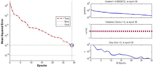
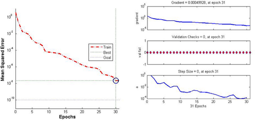
The results of these training methods are summarized in Table 3 and illustrated in Figures 4-6. These visual representations not only highlight the comparative performance of the different methods but also provide a clear understanding of their effectiveness in optimizing neural network training. By examining these figures and the corresponding table, one can observe the nuances of how each method influences the convergence rate, accuracy, and overall efficiency, thereby offering valuable insights into their practical applications in neural network training.
| Method | No. running | Epochs | MSE |
|---|---|---|---|
| HS | 1 | 1000 | 8.74e-06 |
| 2 | 34 | 6.07e-09 | |
| 3 | 41 | 4.40e-09 | |
| 4 | 21 | 5.46e-09 | |
| BIV1 | 1 | 30 | 1.18e-08 |
| 2 | 30 | 1.08e-08 | |
| 3 | 32 | 2.23e-09 | |
| 4 | 11 | 9.10e-06 | |
| BIV2 | 1 | 31 | 2.08e-08 |
| 2 | 33 | 1.08e-08 | |
| 3 | 32 | 4.55e-08 | |
| 4 | 22 | 9.73e-09 |
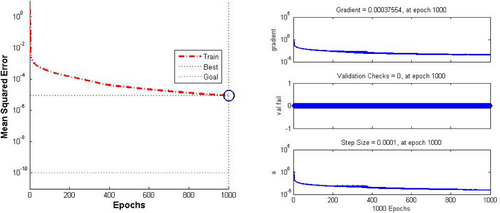
- HS Method: This method shows a wide range of epochs (from 21 to 1000) and varying MSE values, with the lowest being 4.40e-09. However, the high number of epochs in one of the runs (1000 epochs) suggests that this method might not be the most efficient in terms of convergence speed.
- BIV1 Method: The BIV1 method generally requires fewer epochs (between 11 and 32) and produces MSE values that are consistently low. This indicates better efficiency in terms of speed and accuracy compared to the HS method.
- BIV2 Method: The BIV2 method shows a balanced performance, with the number of epochs ranging from 22 to 33 and producing low MSE values. This suggests that the BIV2 method offers a good compromise between speed and accuracy, making it potentially the best overall option for training neural networks in this context.
In summary, while the BIV1 method is faster with fewer epochs, the BIV2 method provides a combination of speed and accuracy, making it a reliable choice for training neural networks.
5 Conclusions
This study presents innovative gradient-based methods, BIV1 and BIV2, designed to improve unconstrained optimization and enhance neural network training. Through rigorous evaluation, the proposed methods demonstrate significant advantages over the traditional Hestenes-Stiefel method. The experimental results reveal that BIV1 and BIV2 achieve superior performance in terms of reduced computational time, fewer iterations, and lower mean squared error during neural network training. The methods' effectiveness is evident across various unconstrained optimization problems, highlighting their efficiency and robustness in high-dimensional scenarios. The BIV1 and BIV2 methods incorporate advanced conjugate gradient techniques that enhance convergence properties and computational efficiency. These improvements are particularly beneficial in training feedforward neural networks, where the optimization process is crucial for achieving accurate and reliable results. The findings underscore the potential of these methods to address complex optimization challenges and contribute to the development of more effective training algorithms for neural networks.
Author Contributions
Bassim A. Hassan: conceptualization, investigation. Issam A. R. Moghrabi: investigation, funding acquisition, methodology. Alaa Luqman Ibrahim: data curation, writing – review and editing. Hawraz N. Jabbar: software.
Conflicts of Interest
The authors declare no conflicts of interest.
Open Research
Data Availability Statement
Data sharing not applicable to this article as no datasets were generated or analysed during the current study.


