Study on Multiobjective Path Optimization of Plant Protection Robots Based on Improved ACO-DWA Algorithm
Funding: This work was supported by Gansu Provincial Department of Education 2013A-114, 23YFFE0001, Tianshui Normal University, CYZ2023-05, CXCYJG-JGXM202304JD.
ABSTRACT
The use of large-scale agricultural machinery for plant protection in nonstandard orchards of mountainous areas is very limited, while small-wheeled robots have great application prospect. To address the false judgment of visual information caused by the shading of branches and leaves and the difficulty in avoiding obstacles in complex orchard terrain, an operation trajectory optimization approach based on the improved dynamic window algorithm (DWA) with ant colony optimization (ACO) was developed. First, the orchard environment information was acquired by laser radar, and the voxel method was used to reduce the point cloud density of orchard ground. The grid method was used to segment the point clouds. Using the K-means clustering algorithm to extract navigation lines of the tree row. Second, combining with the kinematic model and the motion path constraints of robots, a series of candidate trace points were generated using the model-based prediction algorithm (SBMPO). Then, using the improved ACO-DWA algorithm, the robot access cost was integrated into the objective function of the search node, and the path planning was carried out online based on the environment grid map. Finally, in simulation and orchard validation scenes, the effects of this improved approach were checked through the simulation platform Matlab R2021 and ROS2 operating system. Simulation results on Matlab R2021 show that this improved algorithm has an average of 28%, 16% and 37% reduction in three indicators of the travel path, the number of detours, and the calculation time, respectively. In the orchard real-time experiment, compared with other excellent algorithms, the navigation distance error is reduced obviously. These experimental results show that this method would obviously improve the robot access effect in the inner area between the tree row, significantly meet the requirements of high safety and speed level of robots in these scenes. Also, it could be applied in the field such as picking and spraying robots.
1 Introduction
Nowadays, wheeled robots integrated many intelligent technologies such as depth vision, system integration, and trajectory optimization, which have widespread development and application in the military and civilian fields. In recent years, operation trajectory planning and optimization are key issues in these fields. The algorithms used in path search mainly include intelligent algorithms such as the dynamic window algorithm (DWA), the genetic algorithm, the particle swarm optimization (PSO), and the graph-based search algorithms. The prominent feature of DWA is to limit the acceleration and deceleration performance of the robot to a feasible dynamic range in the velocity sampling space. However, in complex dynamic environments, such as when encountering a “C” shaped barrier, it may not be possible to avoid the hazard well. In addition, it may also generate an smoothless path when generating tracks, especially when precise attitude control or complex environment navigation is required. Genetic algorithm is a randomized search method that has evolved from the evolutionary laws of the biological world, which means survival of the fittest, genetic mechanism of survival of the fittest. PSO is a type of swarm intelligence algorithm designed to simulate the hunting behavior of bird flocks. For the graph-based search algorithms, it has two kinds of methods, such as breadth-first search (BFS) and depth-first search (DFS). BFS is realized by queue, first-in first-out, suitable path planning, shortest path but very inefficient. DFS uses stack implementation, first-in last-out. DFS path is often complex, not shortest. In order to promote the computing efficiency of A* operation, a hop search method has been proposed [1], but this method can not ensure optimal global path in complex. The straight-arc strategy has been used to smooth the trajectory [2]. Using the differential methods has reduced the inflection points number, however increased the calculating cost [3]. The heuristic function of A* was optimized, and the selection strategy of key nodes was improved, so the path redundancy points were reduced [4]. The curvature velocity method (CVM) has been proposed [5], where the obstacle avoidance problem with constraints of the velocity and space were described and an objective optimization function considering three factors, such as speed, safety, and path was developed. On the basis of CVM, a more complete DWA algorithm was proposed [6], where the objective function was addressed with three factors, such as heading angle, velocity, and obstacle distance. The trajectory obtained was relatively smooth and effectively solved the problem of detouring around the obstacles. In the operation of the orchard environment, the kinematic constraints of the robots should also be an important factor to be considered, in addition to obstacle avoidance and access cost. Therefore, some scholars have proposed a method of combining path planning with trajectory optimization to optimize the trajectory [7]. Chen et al. used a quadric spline curve to express the shape of trajectory; however, the limitations of the B-spline curve was not suitable for complex conditions [8]. Al et al. used B-spline curve to optimize the global path step-by-step at the corner and represented the global path by the way of straight line, curve, and straight line [9]. Using cubic uniform B-spline curves to describe the forklift path and optimizing the global path shape; however, this method was mainly suitable for simple operation [10, 11].
To address the false judgment of visual information misjudgment caused by the shading of branches and leaves and the difficulty in avoiding obstacles in complex orchard terrain, this article offers an operation trajectory optimization algorithm based on improved ACO-DWA algorithm including extracting orchard environmental information through laser radar, simplifying point cloud density using voxel grid method, extracting navigation lines of the tree row using K-means algorithm, and combining with the kinematic model and the motion path constraints of robots, etc. A series of candidate trace points were generated using the model-based prediction algorithm (SBMPO). Using the improved ACO-DWA algorithm, the robot access cost was integrated into the objective function of the search node, and the path planning was carried out online based on the environment grid map. Finally, in simulation and orchard validation scenes, the effects of this improved approach were checked through the simulation platform Matlab R2021 and ROS2 operating system.
2 Materials and Methods
2.1 Information Identification System in Orchard Environment
This plant protection robot is made up of a distributed pure electric drive chassis, a 16-line laser radar, a GNSS navigation system, a lithium battery pack, and a chassis controller, etc. It is shown in Figure 1.
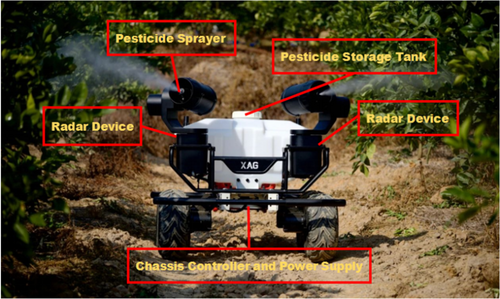
In the orchard environment, the GNSS navigation system serves the robots for global path positioning. The laser radar is used to obtain local environmental information. The size of the robot must meet the requirements between the rows of fruit trees. This is in order to ensure the robot could turn around smoothly during the operation between the rows. The row design width is 100 cm. Most mountain orchards are built according to mountain terrain, and the ground is prone to undulation. In addition, the shading of branches and leaves, the density of trees in the row, and the uneven distribution of orchard light intensity are easy to affect the stability of GNSS signals. These factors will lead to collisions during robot operation. Therefore, in the inner-row of fruit trees, the laser radar would offer the navigation service for local operation path optimization.
2.2 Radar Navigation Process in the Tree Rows
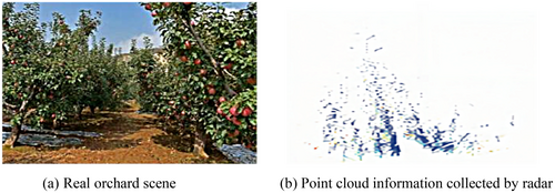
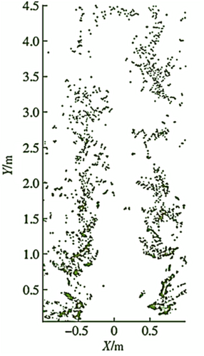
Affected by the shading of branches and leaves and the uneven illumination, actually, in the most areas of the orchard, the distribution of point clouds through radar is more concentrated. The point clouds around it are scattered. However, the area in the middle ground part is significantly smaller than the actual passable size, as shown in Figure 2.
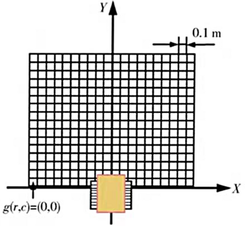
To issue the split task of point clouds, thresholds are applied to evaluate the height difference, height variance, and height gradient of the grid cells. The grid cells are divided into ground areas and other areas. The established ground area projection of the point cloud is shown in Figure 4.
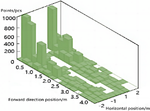
In this article, we use K-mean clustering method to cluster the point cloud in the rows of trees, and the clustering center is used as the backbone area point of the rows. Then, the robot route equation could be fitted.
The point cloud information in the rows of trees obtained by the clustering approach is shown in Figure 5. It can be seen that the point cloud density of the proximal data is higher than that of the far-end data due to the large density of point clouds collected by 16-line laser radar and the lush distribution of branches and leaves.
2.3 Classic ACO Model
The basic principle of the ant colony optimization (ACO) has been explained in detail in [12] and other works. The following paragraph only explained the state transition rate and the pheromone increment model briefly.
2.3.1 State Transition Rate
2.3.2 Pheromone Concentration Update Model
Here, the pheromone concentration updating models are ant density system (ADS), ant quantity system (AQS), and ant cycle system (ACS) commonly. ADS and AQS are applied to the local updating strategy, while the ACS is applied to global update strategy [13]. Considering the computing efficiency and obstacle avoidance ability, this paper uses AQS model as the prototype.
2.3.3 Improved ACO-DWA Algorithm Process
Traditionally, the process of the classical DWA algorithm is to convert the position control into speed control. It describes the obstacle avoidance problems as an optimization problem with constraints in the speed space [16]. The speed space includes the speed, the driving direction, and the position constraints in the surrounding environment.
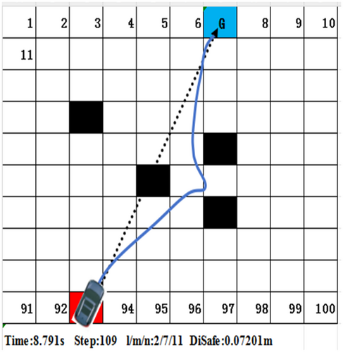
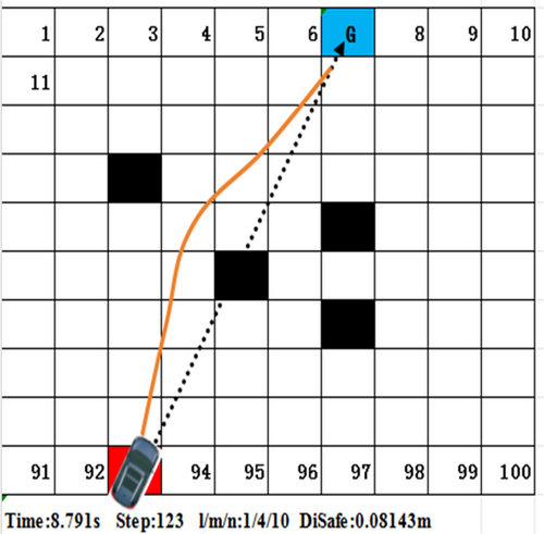
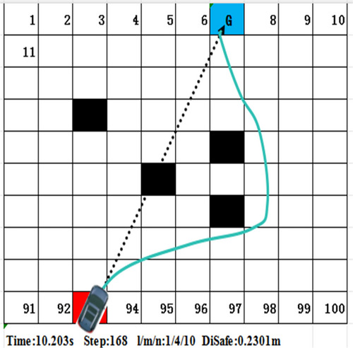
The evaluation function of each possible trajectory node are calculated through Equation (13). We choose the maximum function to the best speed space. Commonly, each weight coefficient in DWA is fixed [20]. Using the voxel grid map to test the approch can be seen that when all the weight coefficients are large [21], the running steps is relatively small, and the computing time is short (as shown in Figure 6). When angle weight coefficient is smaller, the steps is too large and the computing time is long (as shown in Figure 7). When the distance and speed weight coefficients are both smaller, the steps increases significantly and the robot chooses to detours [22]. Meanwhile, the computing time increases significantly (as shown in Figure 8).
Therefore, when a robot is moving at high speed, if the density of surrounding obstacles is too high, the classic DWA will reduce the passing ability. At the same time, the planned path will make the robot too close to the obstacles [23, 24]. Especially when the density of obstacles further increases, the above algorithm will make the robot to go around obstacles. So the path here is too long [25]. In some cases, the path will not be smooth, making the robot to shake between obstacles [26]. The fundamental reason for these problems is that once the weight coefficients are determined, it cannot suitable to different various complex environment. When the environment is changed, it is possible to develop some strange paths which are different to human habits [27, 28].
Based on the above considerations, this article synthesizes the advantages of ACO algorithm globally and continuous search process and develops an improved ACO-DWA algorithm where the weights of evaluation factors are self-adaption through the ACO. It especially reduces the detour distance of robots and improves passing ability and safety in complex and dense obstacle scenes [29].
The specific process of the above weight factors updating based on ACO will be introduced below.
2.3.4 Improved ACO-DWA Algorithm
The high-precision laser radar installed in robots can detect the size and distance information of obstacles in the surrounding area quickly [30, 31]. Assuming at time t, there are certain density obstacles in the surrounding area of the robot as shown in Figure 6.
Then, the feasible solution of this optimization problem is represented by the path of the ants, and all the paths of the whole ant colony constitute the solution space of the optimization. Ants will choose the path with higher pheromone concentration with a higher probability of forming positive feedback. We take the pheromone concentration of the ants as an objective function. The input variable is , and the optimization variable is . Finally, the solution space that satisfies the maximum objective function is the output. The adaptive optimization process of the weight evaluation factors is described as below.
2.3.5 Algorithm Procedure
1st: Environment map information is obtained using high-precision laser radar.
2nd: The starting point, target point, initial heading angle, position, heading, and linear angular velocity are collected.
3rd: The kinematic constraints of the velocity space of the trajectory nodes are determined by the Equations (9-12).
4th: Initialization of ACO parameters.
5th: The solution space is initialized at random. The pheromone concentration is updating according to Equations (14-17). The heuristic information matrix is calculated. The adjacent matrix is queried. The probability that the m-Th ant will choose the adjacent speed state node is calculated according to Equation (11).
6th: The path length of each ant is calculated. The optimal solution (l, m, n) in the current iteration times is recording, which minimizes the evaluation function shown in Equation (13).
7th: Whether to terminate the iteration is a judge: make the number of iterations +1, empty the list of the ant state space, and return to steps 4th–6th. If the value of the evaluation function calculated by Equation (13) becomes larger, terminate the iteration and record the optimal (l, m, n). The population evolution algebra is less than or equal to the maximum evolution algebra G.
8th: The three parts of the evaluation function shown in Equation (13) are normalized. The optimal (l, m, n) is substituted into Equation (13). The corresponding predicted state could be taken into the next original .
9th: The state of the robot speed space is updated. The optimal speed state space is obtained.
3 Results and Discussion
3.1 Parameter Initialization
When the robot faces a unknown environment, the path planning results should be closer to the human riding experience, striving for increased efficiency and convenience. To verify the advantages of this improved algorithm in path planning length, trajectory smoothness, and computing efficiency, this article develops an environment grid map in Matlab and carries out planning experiments on this technology.
In this article, an environment grid map of is constructed as shown in Figure 6. In Figure 6, the red square represents the starting point and the target point, the black squares represent obstacles, and the white squares represent the open space. The square area reflects the expanded size of the robot and obstacles, and the dotted line with an arrow represents the initial start of the planned global path. The colored solid line represents the actual running path.
The parameter settings of the improved DWA algorithm are shown in Table 1. The grid side length is 1. If the expansion radius is 0.5, the robots would collide with obstacles. To ensure that the distance between the robot and the obstacle is not too sensitive and the robot does not bypass, the expansion radius is 0.3 [33]. There are 100 cells in the grid map. Only 1% of the linear speed and angular speed of the robot is taken as resolution. So, each cell can be guaranteed to have a state node. So the resolutions of linear speed and angular velocity are 0.03 and 0.2. According to the level of the initial linear velocity of the robot and the size of the grid map, considering the longest range of path planning, the design simulation test time is 4.
| Expansion radius m | Time resolution s | Resolution of linear speed m/s | Resolution of angular velocity rad/s | Test time s |
|---|---|---|---|---|
| 0.3 | 0.01 | 0.03 | 0.2 | 4 |
The parameter settings of the ACO algorithm are shown in Table 2. reflects the intensity of random factors in the path search. The greater its value is, the more ants will choose the previous path, and the randomness of the search will be weakened [33]. The smaller its value is, the search will fall into the local optimum. According to experience, the general range of the value is [1, 4]. So 3 is chosen in this paper, which has a better comprehensive solution performance [34]. The factor reflects the strength of transcendental and deterministic factors in the process of searching for the optimal path. Based on experience, the general value range is [3, 5]. The size of would affect the convergence speed and global search performance of the algorithm [35]. So it is a number between 0 and 1. According to experience, the value is 0.5. If the number of ant colonies m is too small, the global performance will be reduced and premature stagnation will occur. If m is too large, the convergence speed of the algorithm will slow down. Therefore, based on experience, m generally takes the value of 10–50. The selection of Q is optional without special consideration. The maximum evolutionary algebra G is a parameter indicating the running end condition of the ant colony algorithm, which is generally taken as 100–500.
| G | m | Q | |||
|---|---|---|---|---|---|
| 100 | 40 | 3 | 4 | 0.5 | 100 |
3.2 Discussion
To further verify the solution effectiveness and security of the improved ACO-DWA algorithm proposed in this article, simulation testing of the algorithm is conducted on Matlab R2021 platform here. Simulation testing is performed in three stages: (1) the convergence and global search experiments, (2) the performance test in a grid map environment, and (3) orchard real-time experiments based on the robot ROS2 system.
3.2.1 The Convergence and Global Search Experiments of the Improved ACO-DWA Algorithm
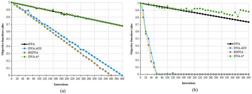
Here, the IEEE CEC2005 benchmark test was used to test the algorithm. The IEEE CEC2005 benchmark test contains 25 test functions including 5 types unimodal functions, 8 multimodal functions, and 12 complex functions. The improved ACO-DWA algorithm in the article was compared and tested with the DWA with fixed weights, DWA-A*, and bidirectional searching DWA (BSDWA). To ensure the objectivity and reliability of the experimental results, the results in the experiment are obtained on the basis of 20 independent runs. The convergence process reflects the optimization details at different stages.
Limited by space, here Figure 9, is showing two representative sets of convergence curves only. The unimodal function f1 tests the convergence performance, and the multimodal function f10 tests the balance ability of the global search and local development. The test results of f1 show that the improved ACO-DWA algorithm performs similarly to BSDWA, with a fast convergence speed, and quickly converges to the global optimum in the early stages of iteration. However, the convergence speeds of DWA and DWA-A* are relatively slow. The test results of f10 show that the improved ACO-DWA performs very similarly to BSDWA, with a very fast convergence speed in the early stages of iteration, which is one order of magnitude faster than the other five variants.
3.2.2 Performance Test in a Grid Map Environment
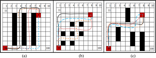
In order to verify the effectiveness of the above improved ACO-DWA algorithm in different scenarios, multiple sets of static obstacle experiments are built in a grid map simulation environment. We compare the differences in path length, smoothness and computing time between these algorithms, and also change the speed and grid map accuracy in three typical static obstacle scenarios. The simulation test results are shown as follows.
As shown in Figure 10, the red line represents the path trajectory of the ACO-DWA algorithm, the black line represents DWA, the blue line represents DWA-A*, and the yellow line represents BSDWA. When we use 10 × 10 grid maps and the robot speed is 10 km/h, it can be seen that there are significant differences in the path trajectories planned. In the circular type, the ACO-DWA and DWA-A* path trajectories are relatively short, with fewer turns and greater fitness with human driving logic. In contrast, BSDWA and DWA prefer to choose a long path when confronting obstacles for the first time. In staggered type, the BSDWA shakes obviously between obstacles. However, the DWA and DWA-A* are obviously longer. In the maze type, there is not much difference in the effectiveness of the four algorithms in the initial stage. However, in the later stage, a more direct way of traveling by ACO-DWA was chosen. So the trajectory of ACO-DWA is the shortest of them. Due to space limitations, the testing path length, number of turns, and computation time in staggered type are shown in Table 3 only. From the below three evaluation indicators, taking DWA as the benchmark, the average enhancement rate of the other three excellent algorithm indicators, respectively, reaches 29%, 22% and 1.8%. So, this improved ACO-DWA is the best of them.
| Parameter | Dist/m | Turning/ number | Computation time/s | aAerage enhancement % |
|---|---|---|---|---|
| DWA | 18.309 | 1 | 1.20 | — |
| Improved ACO-DWA | 14.167 | 2 | 0.78 | 29% |
| DWA-A* | 16.701 | 2 | 0.84 | 22% |
| BSDWA | 17.860 | 4 | 1.19 | 1.8% |
Considering that robot speed is an important variable which affects the algorithm function, this time we choose the speed is 50 km/h. The simulation results are shown in Figure 11.
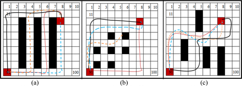
Compared to the results shown in Figure 11, it can be seen that in circular type the DWA chooses a further way to turn less. However, the performance of ACO-DWA has not changed much. In staggered type, the results of these four algorithms have significant changes. To avoid shaking in a staggered obstacle environment at high speeds, ACO-DWA chooses a detour path without turning. In Figure 11b, for the BSDWA algorithm, in order to achieve the goal with the shortest local path, when the robot speed increases and encounters the staggered obstacle environment, it is more inclined to walk between obstacles, which eventually leads to collision with obstacles. In the maze type, DWA has planned a very strange path, and the distance has increased significantly. The other three paths have different degrees of much longer routes. Among them, ACO-DWA has the shortest path. Overall, as the speed increases, the path planned by the ACO-DWA algorithm is relatively short and more suitable to the human driving logic.
3.2.3 Orchard Real-Time Experiments Based on the Robot ROS 2 System
To verify the effectiveness of this algorithm, a physical experiment was conducted in a mountainous orchard in Gansu, as shown in Figure 2. In this orchard, the plant spacing is 20–30 cm, and the row spacing is 65–80 cm. The altitude ranges from 500 to 1000 m, with a relative height of no more than 200 m, and the slope is relatively gentle. The navigation line was planned by defining the communicable area through the central area. Variations in width between 70 and 80 cm had minimal impact on recognition error within the central area.
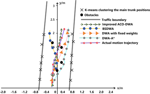
In this experiment, the maximum navigation line error is 5.68 cm, the minimum error is 0.32 cm, and the average error is 3.16 cm. Furthermore, in the physical environment, DWA with fixed weights, DWA-A*, BSDWA, and the improved ACO-DWA are each loaded onto the robot ROS2 system, and the path planning performance is shown in Figure 12. In Figure 12, the cluster centers of fruit trees are extracted using the K-means clustering algorithm, and the row size of fruit trees is determined based on the least squares method, indicated by the black line in this figure. The obstacle positions are marked by black dots. It is observed that the improved ACO-DWA algorithm selected a more direct, non-detour path, while the other three algorithms chose a longer, more circuitous route around obstacles. This trajectory closely resembles the path obtained by controlling the robot between rows of fruit trees via the upper computer, demonstrating the high feasibility. Compared with DWA, DWA-A*, and BSDWA, this improved method has the precision of navigation line planning increased by 18% in average.
4 Conclusions
In this article, a wheeled plant protection robot path planning approach in mountainous nonstandard orchards is proposed. The improved ACO-DWA algorithm supported by ROS2 system can improve the operation efficiency, reduce the detour cost outside the obstacle, and improve the driving safety. The maximum navigation line error is 5.68 cm, the minimum error is 0.32 cm, and the average error is 3.16 cm. The navigation accuracy has improved by an average of 14.2%. Through defining the performance function and considering the obstacle expansion radius, updating the dynamic pheromone model by an optimized ACO, and updating the three weight coefficients of the classic DWA evaluation function as the optimization objective, it is ensure that the robot can arrive at the target point accurately safely and efficiently, especially in complex multiobstacle environment.
Through the convergence and global search performance test, the experimental results show that ACO-DWA has a relatively fast convergence speed and quick converges to the global optimum in the early stages of iteration compared with the classic DWA and the other three excellent transformations of DWA. Through three typical path planning performance tests, ACO-DWA has an excellent performance in both path length, number of turns, and computation time. In staggered type, ACO-DWA has a 14.167 m path length, 2 turnings, and 0.78 s computation time. When the robot speed increases because of the integration of ACO, the global search performance and fast convergence of ACO-DWA are improved. The experiment results show that the robot can still reach the target point with both safety and speed and ensure adaptability and accuracy with the environment transformation. Compared to classic DWA, the improved ACO-DWA in this article is better obviously.
Author Contributions
Jing Niu: conceptualization, methodology. Chuanyan Shen: data curation, writing – review and editing. Lipeng Zhang: funding acquisition, formal analysis. Guanghao Gao: software, writing – review and editing. Jiahao Zheng: formal analysis, writing – review and editing.
Acknowledgments
First of all, I would like to give my heartfelt thanks to all the people who have ever helped me in this paper. This article was supported by Innovation Fund for College Teachers in Gansu Province No. 2013A-114, Key R&D Program of Gansu Province No. 23YFFE0001, Tianshui Normal University Industry Support and Guidance Project No. CYZ2023-05, and Tianshui Normal University Innovation and Entrepreneurship Project No. CXCYJG-JGXM202304JD.
Conflicts of Interest
The authors declare no conflicts of interest.
Open Research
Data Availability Statement
The data that support the findings of this study are available on request from the corresponding author. The data are not publicly available due to privacy or ethical restrictions.


