PD_EBM: An Integrated Boosting Approach Based on Selective Features for Unveiling Parkinson's Disease Diagnosis With Global and Local Explanations
ABSTRACT
Early detection and characterization are crucial for treating and managing Parkinson's disease (PD). The increasing prevalence of PD and its significant impact on the motor neurons of the brain impose a substantial burden on the healthcare system. Early-stage detection is vital for improving patient outcomes and reducing healthcare costs. This study introduces an ensemble boosting machine, termed PD_EBM, for the detection of PD. PD_EBM leverages machine learning (ML) algorithms and a hybrid feature selection approach to enhance diagnostic accuracy. While ML has shown promise in medical applications for PD detection, the interpretability of these models remains a significant challenge. Explainable machine learning (XML) addresses this by providing transparency and clarity in model predictions. Techniques such as Local Interpretable Model-agnostic Explanations (LIME) and SHapley Additive exPlanations (SHAP) have become popular for interpreting these models. Our experiment used a dataset of 195 clinical records of PD patients from the University of California Irvine (UCI) Machine Learning repository. Comprehensive data preparation included encoding categorical features, imputing missing values, removing outliers, addressing data imbalance, scaling data, selecting relevant features, and so on. We propose a hybrid boosting framework that focuses on the most important features for prediction. Our boosting model employs a Decision Tree (DT) classifier with AdaBoost, followed by a linear discriminant analysis (LDA) optimizer, achieving an impressive accuracy of 99.44%, outperforming other boosting models.
1 Introduction
Parkinsonism, generally referred to as Parkinson's disease (PD) is a neurodegenerative condition characterized by a deficiency of dopamine hormone in the brain [1]. This chronic condition leads to severe issues like slow movement, shaking, speech difficulties, and muscle rigidity, with hallmark symptoms being progressive muscle stiffness, tremors, and impaired motor functions [2, 3]. However, PD extends beyond motor dysfunctions, leading to a range of cognitive, sleep, and autonomic disturbances that significantly diminish patients' life events [4]. Cognitive impairments are prevalent in approximately one-third of PD patients, a figure that doubles within 4 years of diagnosis [5]. Among these cognitive issues, dementia is notably common, affecting around 40% of individuals with PD and escalating to 78% after 8 years, a rate significantly higher than that of the general population [6]. Additionally, PD patients often experience challenges with executive functions, attention, spatial awareness, and memory, although these issues are less pervasive compared to dementia [6]. PD diagnosis is typically clinical, relying on a detailed patient history and a thorough neurological examination by specialists [7]. Unfortunately, there is no definitive diagnostic test for precisely identifying PD or any permanent remedy. In low- and middle-income countries, levodopa or carbidopa, the most effective medication for enhancing symptoms, functioning, and quality of life, is not generally accessible, available, or affordable [8].
Over the last 10 years, researchers supported by the National Institute of Neurological Disorders and Stroke (NINDS) have made significant discoveries on the genetic variables that play a role in PD. The genesis of PD is often idiopathic; however, a minority of cases can be ascribed to genetic causes. According to NINDS [9], approximately 15%–25% of individuals diagnosed with PD have a familial susceptibility to the disease. The occurrence of PD resulting from a single mutation in one of many particular genes is exceedingly uncommon. Merely 30% of cases with a family history of PD and three to 5% of sporadic cases those without a documented family history are explained by this. An increasing number of researchers think that both a genetic and environmental component most likely play a role in PD cases if not all of them. Early-onset PD is a very uncommon condition that is more susceptible to hereditary influences compared to the types of illness that occur later in life. Timely identification can improve symptom management and quality of life for PD patients. With increasing PD cases, early detection is crucial. Research indicates that recognizing the condition early enhances treatment outcomes, making it essential to address the growing number of individuals affected by PD promptly. The subtle onset of symptoms makes early diagnosis challenging. An automated machine learning (ML) approach is crucial in this context. ML algorithms have shown great potential in managing large datasets and providing valuable recommendations in the medical field, price prediction, autonomous vehicles navigation, and network attack detection [10-12]. ML technology can enhance patient safety, improve the quality of healthcare, reduce costs, and assist medical professionals in their work. However, effective use of ML technology requires substantial expertise and collaboration. Developing and implementing ML solutions involves meticulous data preparation, finding the right collaborators, and continuous communication between ML experts and domain specialists. ML algorithms in early predictive diseases have proven their capacity to efficiently handle large volumes of data and generate valuable recommendations [13]. Applying machine learning technology can enhance patient safety [14-16], improve healthcare quality [2, 3, 7], reduce healthcare costs, and assist medical workers in their tasks.
Numerous contemporary machine learning models employed in the diagnosis of PD, such Random Forests and Extreme Gradient Boosting (XGBoost), have great accuracy yet function as “black boxes.” This implies that doctors struggle to grasp the predictive mechanisms of these models, rendering them challenging to trust in medical settings where comprehending the rationale behind a diagnosis is as crucial as the diagnosis itself. Selective feature amalgamation in the diagnosis of PD necessitates the examination of diverse data, encompassing motor and non-motor symptoms, vocal analysis, imaging studies, and clinical test outcomes. Current models may neglect the significance of selectively identifying traits that are most pertinent to the condition. This work focuses on the effective selection of characteristics while enhancing interpretability, integrating both global (dataset-wide) and local (individual patient-specific) explanations.
There are a number of obstacles that make early detection of PD challenging. Because most patients are over 60, the time and inconvenience required to diagnose this condition by neurologists and movement disorder specialists who must evaluate the patient's whole medical history can be excruciating. Physicians' domain expertise is crucial for making an accurate Parkinson's diagnosis based on patient data and symptoms. However, there is a severe shortage of qualified medical professionals in many emerging nations, like Argentina, Brazil, India, and so on. Since specialists are already overwhelmed by their duties, making a Parkinson's diagnosis or detection is no easy task. We were inspired to create a decision support system to aid doctors in diagnosing PD because of this. This may be used as a second opinion for Parkinson's diagnosis and, thanks to machine learning, it can help decrease the chance of mistakes.
Despite advances in ML for PD diagnosis, existing models often function as “black boxes,” offering limited interpretability, which hampers their acceptance in clinical settings. Current models, such as Random Forests, XGBoost, and other deep learning methods, while achieving high accuracy, lack transparency and fail to provide clinically actionable insights. Furthermore, few studies leverage selective feature importance tailored for PD, considering both motor and non-motor symptoms. This lack of interpretability and focus on clinically relevant features constitutes a gap in the field, where clinicians need both accurate and explainable models to make informed diagnostic and treatment decisions. Motivated by these gaps, our study introduces PD_EBM, a hybrid boosting model that enhances both accuracy and explainability. By integrating linear discriminant analysis (LDA) for targeted feature selection and Explainable AI (XAI) methods such as SHapley Additive exPlanations (SHAP) and Local Interpretable Model-agnostic Explanations (LIME), PD_EBM aims to bridge these gaps, offering a reliable decision-support tool for early PD diagnosis.
ML models have shown great promise in predicting PD. However, their black-box nature presents a significant hurdle to their adoption in clinical practice. The lack of interpretability and transparency can make medical professionals reluctant to use these models, as understanding the reasons behind a prediction is crucial for making informed treatment and care decisions. Artificial intelligence (AI) stands as one of the most promising domains within computer science, characterized by dynamic research and diverse areas for investigation, particularly in detection and prediction methodologies. Recently, AI's influence has permeated various aspects of daily life, notably catalyzing significant advancements in the healthcare sector.
Although ML-based methods have shown their superiority in illness detection, many of these methods lack the complete interpretability of models for important aspects connected to clinical symptoms in medical data. Therefore, the clinical effectiveness of these methods is still unknown until additional investigations are undertaken to elucidate the key information obtained by these algorithms. To address this, our study indicates the results of the most successful algorithm that employed the LIME and SHAP approaches for XAI. To enhance the applicability of AI in PD diagnosing, it is crucial to offer neuro physicians clear explanations for AI-generated predictions. Understanding the underlying mechanisms that drive these predictions is essential for clinical acceptance and application [17]. Consequently, an XAI framework that integrates the SHAP methodology is necessary to elucidate these decision-making processes. The field of XAI has grown in prominence recently. XAI refers to techniques and methods intended to improve the transparency and interpretability of AI models. Feature significance analysis and saliency maps are two instances of XAI approaches. Among these, LIME and SHAP [18] are particularly popular for explaining ML models in PD prediction. Figure 2 indicates that LIME and SHAP have been utilized in nearly 70% of the studies focusing on PD prediction and interpretation.
- This research proposed an ensemble boosting approach that works on feature importance ensuring efficient and cost-effective analysis.
- This study has the potential to improve patient–physician communication and foster confidence in the model's outcomes.
- The study extends beyond theoretical ML discussions by offering the practical implementation of global and local explainability.
The manuscript is organized as follows: Section 2 provides an overview of the related work. Section 3 demonstrates the existing and proposed methodology. Section 4 outlines the findings and their discussion. Section 5 finally provides a conclusion. The acronyms used throughout the article are tabulated in the Table 1.
| Acronyms | Descriptions |
|---|---|
| AdaBoost | Adaptive boosting |
| DT | Decision tree |
| DFA | Signal fractal scaling exponent |
| GBM | Gradient boosting machine |
| LDA | Linear discriminant analysis |
| LightGBM | Light gradient boosting machine |
| LIME | Local interpretable model-agnostic explanations |
| MDVP: Fo(Hz) | Average vocal fundamental frequency |
| MDVP: Fhi(Hz) | Maximum vocal fundamental frequency |
| MDVP: Flo (Hz) | Minimum vocal fundamental frequency |
| MDVP: Jitter (%), MDVP: Jitter (Abs), MDVP: RAP, MDVP: PPQ, Jitter: DDP | Several measures of variation in fundamental frequency/multiple indicators of fundamental frequency fluctuation |
| MDVP: Shimmer, MDVP: Shimmer(dB), Shimmer: APQ3, Shimmer: APQ5, MDVP: APQ, Shimmer: DDA | Several measures of variation in amplitude/multiple amplitude variation measurements |
| NHR, HNR | Two measures of ratio of noise to tonal components in the voice |
| RPDE, D2 | Two nonlinear dynamical complexity measures |
| Status | Health status of the subject (one)—Parkinson's, (zero)—healthy |
| Spread1, spread2, PPE | Three nonlinear measures of fundamental frequency variation |
| SHAP | SHapley Additive exPlanations |
| XAI | Explainable artificial intelligence |
| XGBoost | Extreme gradient boosting machine |
2 Literature Review
Applying XAI in the detection of various diseases not only improves the precision and effectiveness of diagnosis but also allows for early intervention and tailored treatment approaches. As research advances in this field, the incorporation of explainable artificial intelligence shows significant potential for transforming our comprehension and treatment of disease, ultimately resulting in enhanced patient results. A significant number of researchers have focused their efforts on creating effective XAI algorithms for the diagnosis of disease. Table 2 displays a comprehensive assessment in a tabular format, summarizing the important characteristics, limitations, and methodologies of the pertinent studies.
| Paper | Disease category | Methodology | Findings |
|---|---|---|---|
| Alotaibi et al. [19] | Cirrhosis hepatitis C | Utilize XAI, that is, SHAP and LIME XAI approaches such as SHAP and LIME to pick out the most crucial variables in detecting cirrhosis in patients | The most significant features are RNA 4, BMI, RNA 12, and AST 1, while jaundice and diarrhea are the least significant. Additionally, the prediction probability is 77% |
| Abuzinadah et al. [20] | Ovarian cancer | Implement SHAPly AI method | Observe that HE4 and NEU are prominent features that are highly associated with a substantial percentage of occurrences of ovarian cancer |
| Rikta et al. [4] | Lung cancer | Applies random oversampling and explainable SHAP method | Estimated age, fatigue, chronic disease, and yellow fingers as key contributors for lung cancer and chest pain as least contributing factor |
| Hasan et al. [21] | Hepatocellular carcinoma (HCC) liver cancer | The study utilized the LIME technique to elucidate AI-generated predictions and identify patient-specific responsible genes. | The classification success rate for identifying the first individual as a positive HCC patient is 98% with a confidence level of 98%. Similarly, the second person was categorized as a negative HCC patient with a confidence level of 98%. |
| Ding et al. [22] | Cardiovascular disease prediction | Implement SHAP XAI approach | Exploring the role of residential greenness for cardiac health |
| Khater et al. [23] | Skin cancer | Impose explainable artificial intelligence by utilizing model-agnostic techniques, including partial dependence plots, permutation importance, and SHAP values | SHAP analysis indicates that the asymmetry feature is crucial for predicting melanoma, while the pigment network is significant for identifying nevus of the skin. |
| Islam et al. [24] | Breast cancer | Evaluated the impact of each feature on the model's output and interpreted the predictions of the XGBoost model by applying SHAPly analysis | The mean_perimeter feature exhibits the highest positive SHAP values, signifying that elevated mean_perimeter values significantly aid in predicting early-stage breast cancer. Conversely, the mean_radius feature primarily shows negative SHAP values, indicating that lower mean_radius values are correlated with an increased likelihood of early-stage breast cancer. |
| Chadaga et al. [25] | Cervical cancer | Employ explainable artificial intelligence techniques, including SHAP, LIME, random forest, and ELI5, to enhance model explainability and interpretability | Key factors in the development of cervical cancer include Schiller's test, Hinselmann's test, Cytology test, number of pregnancies, number of STDs, and the duration of hormonal contraceptive use (in years). |
| Arya et al. [26] | Liver cirrhosis | Address SHAP analysis on the proposed XGBoost model | “Cholesterol” has the most substantial impact on the prediction, while “Age” and “Platelets” significantly reduce the influence. |
| Aldughayfiq et al. [27] | Retinoblastoma | Leverage the power of LIME and SHAP, two renowned explainable AI techniques, to create insightful saliency maps | The SHAP algorithm highlighted the existence of a yellow or white mass as a noteworthy characteristic in retinoblastoma. |
| Moreno-Sánchez et al. [28] | Chronic kidney disease (CKD) | Uses local and global interpretation of XAI SHAP method | The hemoglobin feature holds the most significant influence on the probability of chronic kidney disease (CKD), decreasing it with higher hemoglobin values (indicated by red/magenta color) and vice versa. Likewise, elevated levels of the specific gravity feature diminish the likelihood of CKD. Furthermore, the presence of hypertension amplifies the probability of CKD in regression models. |
| Mridha et al. [29] | Stroke | Incorporating SHAP and LIME | As per the SHAP values, six key factors influencing the outcome are age, average glucose level, work type, residence type, gender, and ever married. In a specific instance, the probability of being healthy is 0.01, while the risk of stroke is 0.99. |
| El-Sappagh et al. [30] | Alzheimer's disease | Outline the RF classifier using the SHAP feature attribution framework, which provides both global and instance-based explanations | In each layer's model, we furnished global feature importance for the entire RF model and feature contributions tailored to each individual patient. In the initial layer, our analysis revealed MMSE as the primary predictor for the AD class, while CDRSB emerged as the most influential predictor for CN and MCI classes. In the subsequent layer, FAQ stood out as the most crucial feature for both sMCI and pMCI categories. |
| Magboo et al. [31] | Autism | Implement various machine learning models such as logistic regression, k-nearest neighbors, Naïve Bayes, support vector machine, decision trees, random forest, AdaBoost, XGBoost, and deep neural network along with explainable AI Tool LIME | Support vector machine, logistic regression and AdaBoost provide with 99%–100% accuracy |
The aforementioned articles have significantly enhanced medical professionals' ability to predict life-threatening diseases in their early stages using XAI algorithms. Early detection is crucial to prevent severe complications. Limited significant work has been conducted on neurodegenerative disorders such as PD. Bhandari et al. [32] proposed the Least Absolute Shrinkage and Selection Operator (LASSO) and Ridge regression for feature selection. In their study, they employed advanced machine learning techniques to classify PD cases and healthy controls. Logistic regression and Support Vector Machine (SVM) demonstrated the highest diagnostic accuracy. To interpret the SVM model, SHAP, a global interpretable model-agnostic XAI method was utilized. Nguyen et al. [33] developed a predictive model for depression in Parkinson's disease patients, employing a stacking ensemble approach enhanced by LIME for explainability in the same year 2023.
However, feature optimization methods can improve the results of these algorithms and reduce their computational complexity. Additionally, medical experts often find it challenging to interpret the results generated by these models. Therefore, this research employs XAI methods to ensure that experts can understand the model's outcomes.
3 Research Methodology
In our research, we proposed a PD_EBM framework for Parkinson's disease prediction based on the speech signal features. The suggested framework offers both global and local interpretability, that is, explainable AI to enhance clinical insights into predicting the risk of Parkinson exacerbation. Initially, patient records are gathered and preprocessed. Subsequently, the predictive model is employed to determine the risk of PD disease. Ultimately, the prediction outcomes and their explanations are provided to medical professionals for review and further validation. This research seeks to highlight the essential functions of the LIME and SHAP XAI frameworks in improving the reliability of clinical decision support systems for PD prognosis. The work flow of proposed methodology is illustrated in Figure 1.
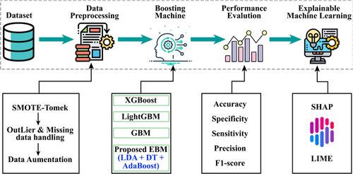
In developing PD_EBM, we aim to address limitations in existing models for PD diagnosis by enhancing both predictive accuracy and interpretability. First, PD_EBM employs LDA for feature selection, optimizing the model to focus on clinically relevant features. This step improves the model's interpretability, as LDA selects features that most effectively separate PD and non-PD cases in a lower-dimensional space, which aligns with clinical reasoning processes. Second, our model integrates Decision Trees (DTs) with AdaBoost, where AdaBoost iteratively corrects errors by assigning higher weights to misclassified cases in each iteration, allowing PD_EBM to achieve high predictive accuracy with minimal false negatives, a critical factor in clinical diagnostics. Finally, by incorporating XAI techniques such as SHAP and LIME, PD_EBM addresses a crucial gap in model transparency. SHAP provides insights into the overall contribution of features to model predictions, while LIME offers localized, instance-specific explanations. These enhancements allow clinicians to understand and trust the model's decisions, making PD_EBM both a powerful and interpretable technique for PD diagnostics.
3.1 Dataset Specification
This study was conducted to anticipate the classification of PD. The dataset was sourced from the renowned PD Prediction dataset from the UCI ML repository [34]. There are 195 instances with 24 features. These features have different interpretations. Firstly, the serial no of instances is in the form of ASCII values. Multi-Dimensional Voice Program (MDVP) represents three types of fundamental frequency in terms of density (Hz) such as MDVP: Fo stands for vocal fundamental frequency (average), MDVP: Fhi stands for vocal fundamental frequency (maximum), MDVP: Flo stands for vocal fundamental frequency (minimum). Then, Jitter is a metric used to quantify the variations in frequency between consecutive cycles, whereas shimmer is a measure of changes in the amplitude of a voice wave. The jitter has three forms collaborating with MDVP. MDVP: Jitter (%), MDVP: Jitter (Absolute), and Jitter: DDP. The Jitter:DDP denotes the average absolute difference of differences between jitter cycles.
The MDVP calculates the amplitude perturbation quotient, five-point period perturbation quotient and relative amplitude perturbation parameters, which are denoted as MDVP:APQ, MDVP:PPQ, and MDVP:RAP, respectively. The MDVP local shimmer parameter is measured in two units: MDVP:Shimmer and MDVP:Shimmer(dB), which represent the original and logarithmic scales, respectively. The initials “Shimmer:APQ3” and “Shimmer:APQ5” stand for the three-point and five-point shimmer perturbation quotient values, respectively. Shimmer:DDA refers to the mean absolute differences in the magnitudes of successive intervals. The acoustic signals' noise-to-harmonics ratio is abbreviated as NHR, while the harmonics-to-noise ratio is abbreviated as HNR. Some examples of nonlinear characteristics include the correlation dimension (D2), recurrence period density entropy (RPDE), detrended fluctuation analysis (DFA), and pitch period entropy (PPE). Two non-linear metrics for measuring variations in fundamental frequency are introduced as Spread1 and Spread2, respectively.
For better classification, the second dataset, meanwhile, was compiled by Sakar et al. [35] from the Department of Neurology at the CerrahpaéŸa Faculty of Medicine, Istanbul University. There were 188 PD patients in this sample, ranging in age from 33 to 87 (10 males and 81 females). This dataset also includes 64 individuals who do not have PD, ranging in age from 41 to 82. There were 23 males and 41 females included in this group. There were 754 characteristics and 756 occurrences in this dataset. For the purpose of this experiment, we randomly divided the two datasets into a training set comprising 80% of the total and a testing set comprising 20%.
3.2 Data Pre-Processing
Outlier detection processes namely z-score [36] and winsorization play pivotal roles in enhancing the accuracy and reliability of disease prediction models. In the context of our proposed PD_EBM model prediction, datasets often contain anomalies or extreme values due to measurement errors, patient heterogeneity, or rare disease occurrences. These outliers can skew the results of predictive models, leading to inaccurate predictions and unreliable risk assessments. By employing outlier detection, researchers and clinicians can identify these anomalous data points that significantly deviate from the normal distribution of patient data. For example, in a dataset predicting the likelihood of a disease like diabetes, outliers might represent atypical cases with extraordinarily high or low glucose levels that do not reflect the typical patient profile. Once identified, these outliers can be addressed using winsorization. Winsorization [37] modifies the extreme values, bringing them closer to a specified percentile within the data distribution. This technique ensures that the impact of extreme values is minimized without completely removing the data points, which could be valuable for understanding the range of disease manifestations. For instance, in the same PD dataset, winsorization might adjust the highest vocal readings to the 95th percentile value, thereby reducing their disproportionate effect on the predictive model.
By integrating outlier detection and winsorization into the preprocessing pipeline, disease prediction models become more robust. This preprocessing step enhances the model's ability to generalize from the training data to real-world scenarios, leading to more accurate and reliable predictions. Consequently, healthcare providers can make better-informed decisions regarding diagnosis, treatment planning, and patient management based on these refined predictive insights.
3.3 Rebalancing Data With Augmentation
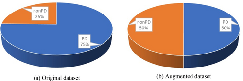
The skew in the sample distribution is termed an imbalanced dataset, which can skew the evaluation results. In this study, a sophisticated data balancing technique, SMOTE-Tomek, was applied to the feature vector to mitigate this issue. This method integrates the SMOTE (Synthetic Minority Over-sampling Technique) with Tomek links under-sampling to enhance the class balance within the dataset. SMOTE operates by producing synthetic instances within the feature space. The fundamental concept of SMOTE involves the generation of artificial samples in the feature space. It randomly chooses a minority class instance and calculates the k-nearest neighbors for this instance [38]. A synthetic sample is then created by selecting one of the k-nearest neighbors and forming a random linear combination of the features from the chosen neighbor and the original instance. SMOTE-Tomek balancing was employed in our analysis to address class imbalance, combining oversampling of the minority class with noise reduction to improve model stability and performance. However, we acknowledge that the synthetic nature of SMOTE-generated samples requires careful validation, especially in clinical applications involving critical decisions, such as drug efficacy predictions or disease progression. In clinical scenarios, data distributions are complex, influenced by factors such as patient demographics, varied disease progression rates, and differing clinical pathways, which synthetic data alone may not fully capture. This limitation could affect the model's generalizability to real-world data. To mitigate these concerns, we validated our proposed model using two separate datasets [34] and [35], where the accuracy results indicate robustness and applicability, ensuring reliable real-world performance. As illustrated in the pie chart, the imbalanced data before and after balancing shows an increase in the minority class (non-PD cases) from 25% to 50% after applying the SMOTE-Tomek technique, while the majority class (PD cases) remains the same.
In some cases, synthetic samples may need to be complemented by additional real-world data collection to ensure model predictions align with actual patient outcomes. We also recognize that synthetic data, while useful, might not fully represent exceptional clinical cases. Engaging clinical experts provides insights into such nuances, ensuring that synthetic data respects biological plausibility and clinical knowledge. Additionally, we further tested our model on a second real-world dataset by Sakar et al. taking these steps to mitigate the risks of synthetic data misrepresenting clinical complexities. By incorporating medically relevant features and validating across datasets, we aim to ensure that our model is both accurate and meaningful in clinical applications.
Using the SMOTE-Tomek data balancing approach, the number of instances increases to 147 for both PD and non-PD classes. Following this, data augmentation techniques such as scaling, rotation, and shifting were employed, resulting in a total of 894 instances. The summary of the data description is shown in Figure 2. Table 3 shows the number of samples before and after the data balancing with augmentation.
| Original data | After balancing | After augmentation | ||||
|---|---|---|---|---|---|---|
| Types | Number | Percentages (%) | Number | Percentages (%) | Number | Percentages (%) |
| PD | 147 | 75.4 | 147 | 50 | 447 | 50 |
| Non-PD | 48 | 24.6 | 147 | 50 | 447 | 50 |
| Total | 195 | 100 | 292 | 100 | 894 | 100 |
3.4 Traditional AI Classifiers Framework
The approach known as boosting [39] is a well-known multiple classifiers learning method that seeks to enhance the performance of machine learning models by successively training numerous weak learners and aggregating their predictions. Iterative training is used to train the sequential base models rather than training the base models separately. This is done so that the models learn to rectify the errors that were produced by the model that came before them during each stage of training. Boosting, which functions as an ensemble meta-algorithm, is able to effectively reduce both bias and variance, which ultimately results in an improvement in the overall prediction performance of PD.
3.4.1 GBM
It is abbreviated as Gradient boosting is an effective approach to machine learning that may be used to solve issues involving classification and regression. Natekin and Knoll described GBM in 2013 [40]. It constructs a model in a stage-by-stage manner, and it generalizes by combining the strengths of several weak learners, which are often DTs. Gradient boosting [41] iteratively adds weak learners to correct the errors of the current model by fitting new models to the negative gradient of the loss function. This approach effectively reduces the loss and builds a strong predictive model by combining multiple weak models.
For each n-dimensional feature vector and as target variables are given in the training dataset is assigned for number of real samples. We introduce a model for predicting given to minimize the expected value of a loss function . We start with an initial model followed by building an additive model where presents the new weak learner added at each iteration To reduce loss at each stage , is added . Gradient boosting uses gradient descent to fit to the negative gradient of the loss function L concerning the current model's predictions . The negative gradient serves as the pseudo-residuals by . Then, we fit to the calculated residuals through the formula and update the final model to where is a learning rate that controls the contribution of each weak learner.
3.4.2 XGBoost
XGBoost used by Dhaliwal et al. [40], is an updated version of the GBM method. It is an iterative process that calculates weak classifiers [4]. Through the integration of regularization, parallelization, improved handling of missing data, various tree-pruning approaches, and integrated cross-validation methods, XGBoost improves the algorithm. Also, XGBoost improves upon traditional gradient boosting by incorporating a regularization term to control model complexity, using second-order derivatives to improve the optimization process, and implementing various algorithmic enhancements for efficiency. The mathematical derivation focuses on minimizing a regularized objective function through a series of additive trees optimized using gradient and Hessian information.
Consider the same feature vector and as the target variable described earlier in the gradient boosting method. Here, specifically, we want to minimize the expected value of a regularized objective function where L is a differentiable loss function and is a regularization term that penalizes the complexity of the model. Next additive model of XGBoost becomes is a new tree weak learner added at each iteration . It is essential to add at every iteration , so objective function turns into . A second-order Taylor expansion to approximate the loss function around as for the first and second derivatives of the loss with respect to the prediction and presented by and , respectively. A tree is regularized by where T represents the number of leaves in the tree, is the weight of leaf , γ is the penalty for each leaf, and λ is the penalty for the leaf weights. Using these, the objective function can be simplified as (ignoring constant term )).
Additionally, be the leaf index of the tree for sample i. Let, the previous objective function becomes be the set of indices of samples in leaf m. Optimizing the weights , set the derivative of with respect to to be zero, . Finally, substitute back into the objective to get the optimal value:
3.4.3 LightGBM
Both LightGBM and XGBoost are gradient boosting frameworks that employ DTs as their basic learners. Although they have a same fundamental idea, they diverge in some crucial respects, such as their methods of tree construction and data handling. More visual representation of tree forming is shown in Figure 3. Osman et al. [42] introduced LightGBM. Mathematically, the objective function in LightGBM combines the loss function L, a differentiable loss function and is a regularized term by the formula Here, the regularized term in LightGBM is defined for a tree can be expressed as . LightGBM grows tree leaf-by-leaf, selecting the leaf with the highest potential split gain. This often results in deeper and potentially unbalanced trees. LightGBM builds the model in an additive manner Each new tree is fitted to the negative gradient (pseudo-residuals) of the loss function . be the pseudo-residuals for the -th sample at iteration . Finally, the overall formula encapsulates the iterative process of building the gradient boosting model with regularization . Then a leaf is split into two child nodes (left and right ), the gain from the split can be calculated as the reduction in loss. The gain from splitting a leaf is given by G = Gain from spilt , where the pseudo-residual for sample and is the second-order derivative (Hessian) for sample . To select the leaf that results in the highest gain from a potential split, we use the operator as . This means that we evaluate all possible leavesluate all possible leaves and choose the one that maximizes the gain . Hence, by iteratively adding trees that fit the pseudo-residuals and selecting the optimal leaf to split, LightGBM efficiently optimizes the objective function with controlled complexity.

3.5 Proposed Methodology
Where vi is the ith eigenvector and λi is the corresponding eigenvalue.
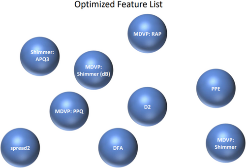
This projection focuses on finding the linear combinations of features that maximizes class separability for the optimal projection of the data; leading to improved classification performance and dimensionality reduction. Figure 4 represents the feature importance outcome using LDA feature vector in the proposed PD_EBM framework.
Where, is the prediction of the base model for the sample , is the true label of the sample , and 1(·) is the indicator function.
Algorithm 1, summarize the working procedures of the proposed PD_EBM in details.
ALGORITHM 1. Proposed PD_EBM.
Input: Dataset
Output: Evaluation metrics (Accuracy, Precision, Recall, F1 Score)
Start
Load Data:
Preprocessed Data:
Standardize Features:
Split Data:
Apply LDA:
Train DT:
Apply AdaBoost:
Evaluate Model:
Hyperparameter Tuning:
Use grid search or random search to find optimal hyperparameters for LDA, DT, and AdaBoost.
End
3.6 XML Algorithms
To foster trust in ML approaches, it is essential to visually illustrate and clarify how ML models arrive at decisions [19]. The use of explainable ML (XML) is critical in ensuring that people can easily grasp both the algorithm's decision-making steps and the data used in its training process [4]. The Explainable Ensemble Machine Learning for Parkinson Disease (XEMLPD) framework incorporates XML techniques such as SHAP and LIME to enhance the transparency and interpretability of ML models' decision-making processes [48]. SHAP can elucidate the model's output by identifying the factors that most significantly influence the prediction of PD. For instance, in a particular patient, the model may forecast a significant probability of PD. The SHAP explanation may indicate that the primary contributing factors include elevated tremor frequency in hand motions, heightened speech abnormalities, and minor alterations in brain imaging consistent with early neurodegenerative indicators. Equipped with this elucidation, the doctor can concentrate on these emphasized characteristics and investigate other diagnostic assessments. If the SHAP explanation indicates that these critical aspects are clinically pertinent to the patient's condition, the doctor may prioritize early intervention or suggest certain medications. If the SHAP readings indicate aspects irrelevant to the patient's current state, the doctor may reevaluate the diagnosis and explore other reasons for the symptoms. Some speculative instances might be used to examine LIME's potential in clinical decision-making. Consider, for example, a model that predicts a patient's risk of heart disease and uses LIME to explain high-risk forecasts. LIME may reveal that the main characteristics influencing the high-risk prediction are age, cholesterol, and family history. This realization might support a clinician's decision to give these risk factors top priority in therapy or additional testing. For instance, the doctor should prioritize dietary and lifestyle modifications before thinking about more intrusive procedures if LIME identifies elevated cholesterol as a significant contributing factor. In this case, LIME promotes a more focused treatment strategy by assisting the doctor in comprehending why the model identified the patient as high risk.
3.6.1 SHAP
SHAP is a method for explaining individual predictions of machine learning models based on cooperative game theory [49]. In cooperative game theory, the Shapley value is a method to fairly distribute the “payout” among players based on their contribution to the coalition. In the context of SHAP, each feature in a prediction is considered a player, and the payout is the difference between the prediction for a specific instance and the average prediction for all instances [50]. SHAP considers all possible subsets of features (coalitions) and calculates the contribution of each feature to the prediction by measuring the change in prediction when that feature is included in the coalition.
The magnitude of SHAP values quantifies the influence of each feature on the PD prediction. Positive SHAP values indicate that the presence of a feature increases the PD prediction relative to the average prediction, while negative SHAP values indicate the opposite influence.
3.6.2 LIME
The feature importance is obtained from the attributes of the local model g. This will generate an explanation by highlighting the most influential features and their contributions to the prediction. This can be written as Explanation(x) = Feature Importance(g).
4 Result and Discussion
This process will yield a total of 894 instances in the working dataset, randomly divided into 715 (approximately 80%) for training and 178 (approximately 20%) for testing purposes. The proposed boosting model reaches the highest performance results compared with the existing boosting methods. To obtain the results, various environments were employed in this study. Table 4 outlines the environment setup necessary for the experiment. All techniques were executed on a local machine using Jupyter Notebook in Python, utilizing libraries or modules such as Scikit Learn, NumPy, Pandas, Seaborn, and Matplotlib.
| Resources | Details |
|---|---|
| GPU | Nvidia K80 |
| GPU memory | 16 GB |
| CPU | Intel Core i5-12600K @ 3700 MHz |
| RAM | 64 GB |
| Cache | 128 MB |
| Disk space | 500 GB |
| Session | 12 h |
Here, the confusion matrix consists of the following terms
| Predicted Positive | Predicted Negative | |
|---|---|---|
| Actual Positive | TP (True Positive) | FN (False Negative) |
| Actual Negative | FP (False Positive) | TN (True Negative |
The comparative performance of GBM, XGBoost, LightGBM, and our proposed EBM method in identifying PD and non-PD patients reveals distinct differences in their evaluation metrics in Figure 5. The EBM exhibited no false negatives (FN) which is a crucial factor in healthcare diagnostics. In contrast, other boosting techniques GBM, XGBoost, LightGBM presented identical FN counts, that is, 2. Remarkably, GBM, XGBoost, LightGBM presented FP of 2, 4, and 1, respectively while proposed EBM had the only 1 (FP which indicates the model's sustainability).
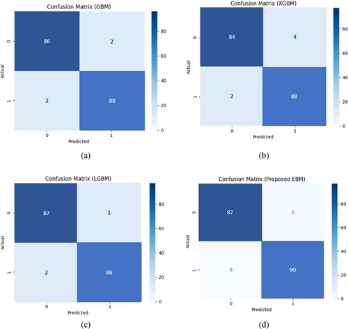
The critical balance between reducing false negatives (FNs), which are pivotal for accurate patient diagnosis, and minimizing false positives (FPs), essential for preventing unnecessary medical interventions, is paramount. Misdiagnosing PD not only wastes medical resources but also adversely affects patient mental health. Therefore, an optimal model must judiciously manage the trade-off between FPs and FNs. In this regard, the proposed Boosting Method (EBM) demonstrated superior performance compared to other models in detecting PD patients. As illustrated in Figure 5, the EBM effectively minimizes both FPs and FNs, outperforming XGBoost, GBM, and LightGBM in descending order. Additionally, GBM, XGBoost, and EBM reported adverse false diagnosis rate (FN and FP). Furthermore, XGBoost had the lowest number of true positives (TP), followed by GBM and LightGBM accordingly while our proposed EBM achieved the highest TP and TN values. Overall, quantitative outcome of evaluation metrics is presented in Table 5 that indicates EBM surpassed other models in accurately detecting both PD and non-PD patients. Table 5 shows the comparative results of different boosting models using two different datasets. We have re-evaluated our experiment with two new datasets to check the generalizability of proposed EBM. It reduces overfitting and computational complexity by preserving the most discriminative features, thus giving higher predictive accuracy.
| Methods measurements | GBM | XGBoost | LightGBM | Proposed EBM | |
|---|---|---|---|---|---|
| Max Little Dataset total instances = 195 | ACC | 97.75 | 96.63 | 98.31 | 99.44 |
| SPE | 97.78 | 97.78 | 97.78 | 100.00 | |
| SEN | 97.73 | 95.45 | 98.86 | 98.86 | |
| PRE | 97.73 | 97.67 | 97.75 | 100.00 | |
| F1 score | 97.73 | 96.55 | 98.30 | 99.43 | |
| Sakar et al. dataset total instances = 756 | ACC | 96.45 | 95.63 | 97.91 | 99.14 |
| SPE | 97.38 | 97.78 | 98.38 | 100.00 | |
| SEN | 96.93 | 95.25 | 98.86 | 98.06 | |
| PRE | 97.50 | 97.27 | 97.35 | 100.00 | |
| F1 score | 97.48 | 96.15 | 98.10 | 99.03 |
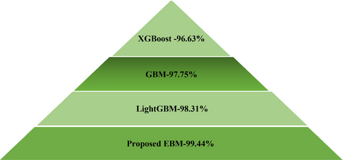
The comparative study is depicted in a pyramid in Figure 6 for Max Little Dataset. Since accuracy is a dependable measure for balanced datasets, it was selected as the primary performance metric for this experiment. The findings showed that the proposed EBM classifier outperformed all other models with an accuracy of 99.44%. In contrast, the XGBoost classifier had the lowest performance across all metrics. Among the classifiers evaluated, LightGBM achieved the second-highest rank, while GBM secured the third position in terms of accuracy. Ultimately, our proposed Explainable Boosting Machine (EBM) achieved the highest balanced accuracy in this study.
We use 10-fold cross-validation to obtain performance scores for both the XGBoost model and the DT baseline model. A paired t-test compares the two sets of scores to check if the difference is significant and tabulated the results in Table 6. Also, a p-value below 0.05 indicates statistical significance, suggesting the improvement is not due to random chance. Accompanying each model's t-statistic, the model provides a p-value, which quantifies the probability that observed differences in model performance occurred by chance. Here, each model has a p-value below 0.05 (e.g., 0.005 for GBM, 0.009 for XGBoost), suggesting a high degree of confidence that the performance differences are significant.
| Methods | GBM | XGBoost | LightGBM | Proposed EBM |
|---|---|---|---|---|
| Measurements | ||||
| t-statistics | 3.15 | 3.57 | 3.31 | 3.67 |
| p | 0.005 | 0.009 | 0.013 | 0.012 |
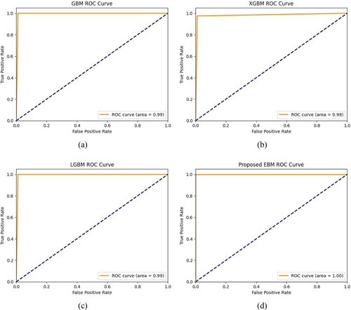
This study employed another performance metric, namely the AUC-ROC curve, to analyze the effectiveness of the proposed experiment. The ROC [38] curve is a vital tool in assessing the performance of disease prediction models. By analyzing the trade-offs between sensitivity and specificity across different thresholds, healthcare professionals can select the most appropriate model for early and accurate disease detection, ultimately improving patient outcomes. To visualize the false positive rate (FPR) in relation to the true positive rate (TPR) is through the Area Under the Receiver Operating Characteristics Curve, also known as AUC-ROC. The AUC-ROC value measures the model's ability to differentiate between PD and non-PD cases, providing an overall prediction score for the EBM algorithm. An AUC score of 0.00 indicates completely incorrect predictions, while a score of 1.00 signifies perfect accuracy.
Figure 7 presents the AUC-ROC curves for different Boosting methods applied with feature selection in the proposed EBM model. The findings indicate that the Boosting classifiers, namely GBM and LightGBM exhibited an upward trend in performance, with AUC-ROC values of 0.99 while XGBoost shows slight downward of 0.98. Notably, the EBM model achieved an outstanding AUC-ROC score of 1.00 in the prediction outperforming other three models.
4.1 Explainability and Visual Explanation of This Experiment
The concept of XAI has been recently introduced to enhance the reliability of AI-based predictions for PD. XAI encompasses various machine learning techniques designed to create models that address the growing demand for transparency and explainability in healthcare. These techniques allow people to understand, trust, and manage the latest AI models. Two frameworks, in particular, are recognized as leaders in the field of XAI. One is SHAP values, developed by Lundberg et al., which provide consistent and accurate attributions for each feature in a model, explaining their contributions to specific predictions. The other is LIME, developed by Ribeiro et al., which clarifies the predictions of any machine learning model by approximating it locally with an easily understandable model.
To explore the process of PD classification in greater detail, we will examine three SHapley additive theories that are relevant to clinical data analysis. Figure 8 presents the SHAP values impact on the model output of the Beeswarm distribution for the top 10 influenced features, arranged in descending order, regarding the prediction PD and Non-PD classes. The Beeswarm scatter plot effectively illustrates the relationship between selected features, resolving data overlap by spreading out multiple individual assessments. The x-axis represents data points, while the y-axis shows the average data density. In our detailed analysis, features with lower impact are indicated in blue, those with increasing impact in purple, and the features with the highest impact in red.
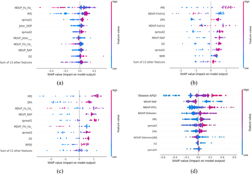
Figure 8 depicts four models: GBM, XGBoost, LightGBM, and proposed EBM. The analysis identifies Shimmer and MDVP as the primary features influencing the Explainable Boosting Machine (EBM) model's predictions for PD. As the density of red values for these features increases, their impact on the model's predictions strengthens. Conversely, a decrease in blue feature values, such as spread2, DFA, MDVP(dB), D2, and spread1, lessens their influence. Additionally, features like MDVP, PPE, and Shimmer significantly enhance the performance of the models under consideration, as evidenced by a high frequency of red data points. Conversely, the D2 metric influences the classification of PD and non-PD subjects for both the GBM and the newly proposed EBM methodologies. Meanwhile, NHR and RPDE exhibit a detrimental effect, indicated by the substantial number of blue data points.
This research shows how to measure each feature's contribution to achieve optimal accuracy and identify the most important features that influenced the PD prediction. Each model exhibits unique importance for different features. For GBM, as illustrated in Figure 9a, MDVP:Fo and PPE are the most important features with absolute SHAP value of +0.1 that significantly exceeds the all other features. Spread1 is the second most influential feature, contributing +0.04. Similarly, Jitter:DDP, Spread2, MDVP:Jitter (%), MDVP:Fhi(Hz), and MDVP:RAP exhibit the same absolute SHAP values of +0.03 while D2 score is +0.02. The combined impact of 13 features on PD detection is minimal, summing approximately +0.08.
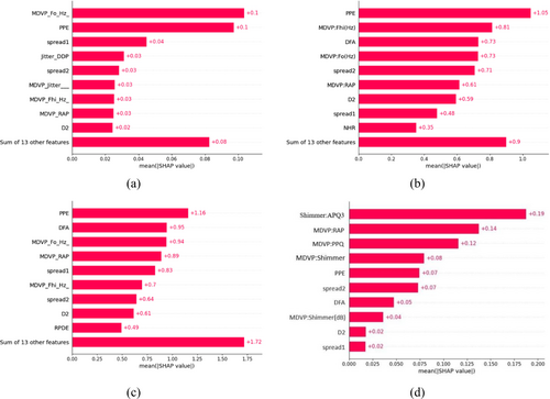
In Figure 9b,c, the case of XGBoost and LightGBM apparently, shown that PPE is the primary contributor, accounting for +1.05 and +1.16, respectively. MDVP:Fhi being the second most important for XGBoost while DFA serves same position for LightGBM. In Figure 9b, The descending order of feature importance is DFA >MDVP:Fo > spread2 > MDVP:RAP > D2 > spread1 > NHR for XGBoost. Similarly in Figure 9c, MDVP:Fo >MDVP:RAP > spread1 > MDVP:Fhi > spread2 > D2 > RPDE for LightGBM. The other 13 feature have less contribution for both three models.
Our proposed EBM model selects features in a slightly different manner. The bar diagram highlights 10 features obtained after feature optimization. In Figure 9d, the features are ranked in descending order based on their importance as: MDVP:RAP>MDVP:PPQ>MDVP:Shimmer>PPE and spread2 > DFA>MDVP:Shimmer (dB > D2 > spread1for EBM whereas Shimmer:APQ3 is the leading feature). Thus, the EBM proves noteworthy in demonstrating that it works well for explaining features effectiveness.
Waterfall plots illustrate the impact of each feature on the PD forecast. In our study, the “SHAP Waterfall Plot” illustrates the enumeration of attributes on the x-axis and the display of SHAP values through bars that extend from the baseline (usually zero) to the final prediction. Positive SHAP values indicate that a feature positively influenced the forecast, while negative values indicate that it had a negative impact on the prediction. The height of each bar represents the contribution of the characteristic to the forecast. It facilitates a clear understanding of how each characteristic influences prediction and interacts with one another. It aids in identifying the most significant qualities, assessing their positive or negative effects, and understanding their impact on the final prediction. Figure 10, displays waterfall graphs for GBM, XGBoost, LightGBM, and EBM respectively.
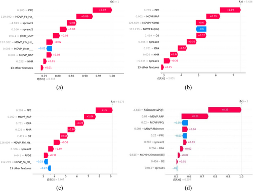
The SHAP value measures the individual impact of each feature on the prediction of each class. Figure 10 illustrate that the same variable “PPE” at first position has a positive SHAP value of 0.07, 1.19, and 1.5 for GBM, XGBoost, LightGBM relatively. Conversely, the variable “MDVP:jitter (%)” has a negative impact on the GBM model, while MDVP:Fo gives negative value for both XGBoost and LightGBM. The sum of all SHAP values is equal to the difference between the Ef(x) and f(x). The presence of PPE and MDVP:PPQ have a detrimental effect on the prediction for Figure 10d, whereas presence of Shimmer:APQ3 and MDVP:RAP claims a significant favorable impact on the prediction of Parkinson's disease.
Thus, our predicted EBM model proves its importance in terms of both accuracy and SHAP explanations.
Figure 11 illustrates the LIME explanation. Orange bars represent the medical background and symptoms that heavily support the prediction, while blue bars indicate factors that argue against it. This LIME XAI method clarifies the expected results of the four models. Consider a Gradient Boosting Machine (GBM) and an Extreme Gradient Boosting Machine (XGBoost) at first. They share similar results. Specifically, the upper left part of Figure 11a,b shows that the prediction score for patients diagnosed with positive PD cases is 100%, and for negative PD cases, it is 0%. The explanation says that at the time of prediction, the patient's voice signal features that helped for GBM model with the prediction were MDVP_Fhi_Hz and MDVP_Flo, D2, and some other features that aren't seen as often in Parkinsonism diagnoses. This implies that MDVP_Fhi_Hz (126.61) is positively skewed, whereas MDVP_Flo (104.09) and D2 (2.42) fall within the ranges of 86.56–116.21 and 2.34–2.63, respectively. In contrast, MDVP_Fo (112.24) and HNR (17.34) rule out the negative class prediction of Parkinsonism. Also, for XGBoost the feature importance is relatable to GBM approximately.

Next, let's examine the LightGBM model. As illustrated in Figure 11c, it achieves a prediction score of 99% for patients diagnosed with positive PD cases and 1% for those with negative PD cases. This suggests that LightGBM performs slightly better than both GBM and XGBoost. The explanation reveals that during the prediction process, the patient's voice signal characteristics, specifically MDVP_Fhi_Hz and MDVP_Fo, were less useful for predicting Parkinsonism. Notably, MDVP_Fhi_Hz (126.61) exhibits a negative skewness, which contrasts with the results from the GBM and XGBoost models. Interestingly, while the feature values are consistent with those of the other two models, the impact of MDVP_Fhi_Hz on prediction effectiveness is reversed.
Finally, we are considering the implementation of our suggested Explainable Boosting Model (EBM). Figure 11d exhibits notable disparities when compared to the other three models. In particular, the prediction score is 51% for patients classified as having positive PD and 49% for those classified as having negative PD. It suggests that the EBM is more trustworthy than GBM, XGBoost, and LightGBM when it comes to predicting probabilities. The patient's speech signal features that were very informative for generating the prediction were MDVP:PPQ, Jitter:DDP, MDVP:Shimmer, and MDVP:Shimmer in decibels. Likewise, MDVP: Jitter in percentage made a considerable contribution to recognizing the positive class of Parkinsonism diagnosis. The figure also indicated that the MDVP:Flo and MDVP:Jitter values provide evidence that Parkinsonism is absent.
However, extensive research has been conducted on this subject by numerous researchers using various methods, resulting in a range of findings. Accurate PD forecasting is crucial, as Parkinson's affects people worldwide. The significance of Parkinson's motivated us to explore this topic. This study focuses on using XAI to forecast Parkinson's and demonstrates a practical implementation that can predict PD or non-PD based on given inputs. Table 7 provides a comparison of this work with previous research to understand the existing knowledge on the topic and identify gaps in the literature that this study can address.
| Paper | Model | Classes | Accuracy (%) | Precision (%) | Recall (%) | F1 score (%) |
|---|---|---|---|---|---|---|
| Senturk et al. [53] | LightGBM | PD/non-PD | 95 | 93.3 | 100 | 90 |
| Celik et al. [54] | MLP | PD/non-PD | 98.31 | 100 | 98 | 99 |
| Solana et al. [55] | XGBoost + RF | PD/non-PD | 94.89 | 93 | 93.22 | 93.11 |
| Nahar et al. [56] | Gradient boosting | PD/non-PD | 77.21 | 79 | 72 | 78 |
| Polat et al. [57] | SMOTE + RF | PD/non-PD | 94.89 | 95.1 | 94.9 | 94.9 |
| Nissar et al. [1] | XGBoost + mRMR | PD/non-PD | 88.82 | 88 | 89 | 88 |
| Mahesh et al. [58] | XGBoost + SMOTE + RF | PD/non-PD | 98.00 | 97.24 | 97.56 | 97.40 |
| Oguri et al. [59] | LightGBM + GBM + DT | PD/non-PD | 97.43 | 96.82 | 100 | 98.38 |
| Lshammri et al. [60] | MLP + SMOTE + GridSearchCV | PD/non-PD | 98.31 | 100 | 98 | 99 |
| Rehman et al. [61] | Hybrid LSTM + GRU | PD/non-PD | 98.00 | — | — | — |
| Al-Tam et al. [62] | Stacking | PD/non-PD | 96.05 | — | — | — |
| Bukhari et al. [63] | SMOTE + PCA + AdaBoost | PD/non-PD | 96 | 98 | 93 | 95 |
| Proposed | LDA + DT + Adaboost | PD/non-PD | 99.44 | 100 | 98.86 | 99.43 |
- Note: Bold values indicate the height value.
In summary, the experimental results demonstrate that PD_EBM achieved the highest accuracy of 99.44%, with a sensitivity of 98.86% and specificity of 100%, F1 score 99.43%, outperforming GBM, XGBoost, and LightGBM across all metrics. This performance highlights PD_EBM's effectiveness in minimizing false negatives, which is crucial in clinical applications where misdiagnoses can have severe consequences. Additionally, PD_EBM's integration of SHAP and LIME provides valuable insights into feature importance and individual predictions, supporting clinical interpretability. These findings underscore PD_EBM's potential as a reliable decision-support tool, balancing accuracy and explainability, thus making it well-suited for practical applications in PD diagnosis.
5 Conclusion
This study underscores the effectiveness of XML in identifying PD using minimal tests or features. For early detection, we employed various boosting algorithms, including Gradient Boosting, XGBoost, and LightGBM. We introduced a hybrid boosting framework called PD_EBM, which leverages the most significant features to enhance PD prediction accuracy. The PD_EBM framework achieved outstanding results in distinguishing between PD and non-PD cases, with an accuracy of 99.44%, a specificity of 100%, a sensitivity of 98.86%, a precision of 100%, and an F1 score of 99.43%, surpassing the performance of other models. These findings suggest that ML-based boosting models can be pivotal for resource development and public health initiatives, such as continuous patient monitoring and early PD detection. Throughout this research, we utilized explainable AI techniques like LIME and SHAP to elucidate the complex ML models. LIME provided localized explanations for PD classifications based on individual instances, while SHAP, grounded in cooperative game theory, offered deeper insights into model predictions using patient data. Both techniques significantly enhance the transparency and trustworthiness of the models, which is crucial for their application in real-world settings, particularly in healthcare data analysis. As explainable machine learning evolves, LIME and SHAP will continue to play key roles in improving the interpretability and accountability of ML models, ensuring they remain reliable tools in clinical decision-making. Our future study will concentrate on different ensemble machine learning models and feature selection techniques in addition to including new data sources. In order to offer more thorough insights into the prediction process, the models' interpretability could also be improved.
Author Contributions
Fahmida Khanom: writing – original draft, formal analysis, data curation, resources, visualization, methodology. Mohammad Shorif Uddin: writing – review and editing, project administration, validation, supervision. Rafid Mostafiz: conceptualization, investigation, methodology, visualization, supervision, data curation, validation.
Conflicts of Interest
The authors declare no conflicts of interest.
Open Research
Data Availability Statement
The dataset used in this work has been deposited into a publicly available UCI Machine Learning repository. The dataset can be accessed via the link: https://doi.org/10.24432/C59C74 and the second dataset can be accessed via the link: https://doi.org/10.24432/C5MS4X.


