The increasing occurrence of severe droughts and sparse rainfall due to climate change is resulting in high and costly demand for water resources. A greater understanding of uncertainties associated with the creeping occurrence of agricultural drought and proactive planning to mitigate drought impact hence needs a probabilistic assessment. This study presents the probabilistic characterization of agricultural drought, depicted by the cumulative soil moisture deficit above a threshold (Severity) and water stress in the plants (WSP-sum) during dry periods (duration). The concept of Crop Growing Process (CGP) for specified crops is introduced and defined as a continuous flow of water from the soil through the roots of the plant to the leaves then transformed into water vapor and finally released. The CGP is a two-state process, either a normal or subnormal state. The probability density function (PDF) of the WSP-sum manifests the overall subnormal state of CGP over the duration by means of the failure probability estimated as the sum of two distinct parts from two independent phases. Phase1 estimates the part of the failure probability influenced by the average duration; and Phase-2 estimates the remaining part influenced by the average severity. The phase with the smallest rate parameter determines the WSP-sum, which indicates whether a premature end of CGP was due to drought or the CGP survived until the end of the cropping season. The predicted designed drought components for specified return periods are presented to assist in proactive drought management. The combined influence of all the drought components upon the WSP-sum probabilistically characterizes agricultural drought, given the CGP.

1 INTRODUCTION AND OBJECTIVES

Extreme drought events are becoming increasingly frequent, severe and costly mainly due to sparse or absent rains, variability in hydro-meteorological variables arising from the climate change. The significant impact of drought upon crop production, local economies, water availability, and land factors is contributing to desertification.1, 2 A greater understanding and investigation of drought events is becoming important for water resources planning and developing drought impact mitigation strategies.3, 4

This paper presents the probabilistic characterizations of agricultural drought, introducing the concept of Crop Growing Process (CGP), which is a two-state process, either normal or subnormal state. The CGP for a specific crop or a group of crops is regarded as the evapotranspiration, which is a continuous flow of water in the soil transferred through the roots of the plants to the leaves, where it is transformed into water vapor and finally released into the atmosphere.5 The degree of subnormal sate of the CGP depends on the transpiration rate and the level of water available in the soil for absorption.6 Doorenbos and Kassam7 classified several crops into four groups based on the above concept of soil-water depletion and the yield response of crop(s) within a group to the soil-water available for CGP. Crops within a group are assumed to have similar root zone, crop coefficients, yield response, crop-water need and other such factors.8 The subnormal state (or failure) of the CGP consisting of one or more crops is determined by the water stress in the plant (WSP), resulting in yield loss or wilting of the crop. This concept is similar to the failure of one or more components within a mechanical device due to some reasons (called hazard).9-11 In the present context, the CGP (like a device) consists of one or more corps (like components) may become subnormal (failure) due to water stress in the plant (like hazard). Surprisingly, no study on agricultural drought has attempted to view CGP from this perspective. A greater understanding of the CGP from this perspective is important to measure the economic impact of agricultural drought events in terms of a substantial crop production loss due to water stress in the plants within a large area of land.6, 12, 13

Most studies on stochastic aspects of droughts applied the goodness of fit and other tests for choosing probability distributions of the components defining drought events as in Figure 1 and generating long historic records containing several drought events. The goodness of fit and other tests have wide applications but the exact distributions of components, if available, are expected to provide better estimates of the generated data.14, 15 This is because, the exact distributions take hydrological reality into account (a top-down approach), which is not necessarily the case for the distributions selected on the basis of the goodness of fit tests (a bottom-up approach).16

Details are in the caption following the image — **Figure 1**
Open in figure viewer PowerPoint

Probabilistic characterization of drought Adapted from Reference 14

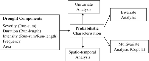
The failure (or hazard) rate function of system reliability and the exact probability distributions of the components of drought events are explored in this study to present the probabilistic characterizations of agricultural drought. Procedures developed in this study are applied to potato production data in East Anglia, England as a case study.

The paper is organized as follows: Section 2 presents definitions of the drought components and literature review; Section 3 estimates the monthly maximum and actual evapotranspiration and soil moisture deficit (SMD); Section 4 presents the probability density function (PDF) of SMD; Section 5 computes threshold SMD (TSM) and its PDF; Section 6 presents the PDF of (SMD-TSM); Section 7 computes drought duration (run-length), severity (run-sum) and the total water stress in the plant (WSP-sum) for each of the observed drought events; Section 8 presents PDFs of run-length and run-sum; Section 9 derives the PDF of WSP-sum and the failure rate function of CGP; Section 10 presents procedures for the estimation of the expected run-length, run-sum and WSP-sum of designed droughts for a set of specified return periods; Section 11 discusses the results obtained from the study and draws conclusions and finally recommends a topic for further research.

2 AGRICULTURAL DROUGHT: DEFINITIONS AND LITERATURE REVIEW

2.1 Definitions

Following on from Yevjevich,17 this study assumes that agricultural drought occurs, when the available soil-water cannot sustain the crops' evaporative demand due to a significantly high soil moisture deficit (SMD mm), resulting in a significantly less actual evapotranspiration (Ea_t) than the maximum crop water need (Em_t) during time t (month). If it is possible to compute a target or threshold SMD (TSM in mm) level with a tolerance limit of SMD, so as to increase the harvested actual yield of the crop to a specified proportion of the maximum yield (tons/ha) for a given CGP, which may require additional water supply, then:

Condition 1.(SMD-TSM)>0 measures the soil-water deficit above the TSM during time t (month).

Condition 2.(Em-Ea)>0 measures the corresponding water stress in the plant (WSP) during time t for that CGP.

The CGP relies on many agronomic factors, which are not visible. The variables, (SMD-TSM) and (Em-Ea) are visible and measurable proxy indicators, monitoring the state (normal or subnormal) of the CGP at different stages over its lifetime. From Conditions 1 and 2, the CGP is in subnormal state (failure), when (SMD-TSM)>0 and the corresponding (Em-Ea)>0, otherwise the CGP is in normal state (success) during time t. The concept of subnormal or normal state of CGP is similar to that of the Bernoulli variables in system reliability.9 The sum of consecutive (SMD-TSM) > 0 over the drought duration T (run-length) is the total amount of soil-water shortage (run-sum or severity) relative to cumulative TSM over the run-length, T of the drought as in Figure 2.17 Similarly, the corresponding total of consecutive (Em-Ea)>0 over the run-length, T measures the total amount of the crop-water stress (WSP-sum) during drought.

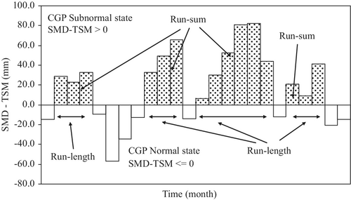
Replacing (SMD-TSM) in Figure 2 by (Em-Ea), would produce a similar picture for the WSP-sum over the same run-length and indeed the normal and subnormal state of CGP. The probabilistic characterizations of the agricultural drought components (Figure 1) are derived from:

the marginal PDFs of SMD, TSM, (SMD-TSM), when (SMD-TSM)>0 and (SMD-TSM)<=0,
the marginal PDFs of run-length, run-sum and WSP-sum.

The WSP-sum is likely to increase with increase of run-length and/or run-sum during droughts. In other words the WSP-sum is expected to be positively correlated with run-length and run-sum. The relationship of WSP-sum with run-length and run-sum is defined by a statistical function, called the “Stress function.” The Stress function estimates the extent of variations of WSP-sum explained by run-length and run-sum during droughts. Finally, the marginal PDF of WSP-sum is derived considering effects of the Stress function and the joint distribution of run-length and run-sum. The failure or nonexceedance probability of the WSP-sum less than a magnitude estimated from the PDF of WSP-sum, which determines the likelihood that the CGP is in subnormal state.

The probabilistic characterizations of agricultural drought are depicted by the:

run-length, run-sum, WSP-sum, return period, failure probability and the failure rate function of the subnormal CGP of observed droughts as well as
expected run-length, run-sum and WSP-sum estimated from designed droughts for a set of specified return periods.15, 18

The above procedures are applied to early-potato and maincrop-potato production data in East Anglia, England. The dry period/drought events are identified from the monthly reference evapotranspiration (ETo) and rainfall (RF) data (1969-1983) available from the Meteorological Office, UK. The agriculture and irrigation in East Anglia during the study period are documented in Dent and Cook.19 The crop (potato) related data are available from Doorenbos and Kassam.7 The cultivation of early-potato and maincrop-potato extends from April-June and June-August/September.20, 21 The agricultural land classification in England and Wales with a brief note of the classification is presented in Figure 3.22 East Anglia is the driest part of Britain and contains large proportion of Grade-1 land as in Figure 3. The average effective rainfall is only about 147 mm/year compared to 487 mm/year for the rest of England and Wales. Evaporation exceeds water demand, resulting in a high soil-water shortage during the summer in East Anglia. About one-third of water used for agriculture is privately abstracted by farmers.21

2.2 Literature review

The review mostly includes recent literature on the probabilistic characterizations of drought as in Figure 1. Since the publication of Yevjevich,17 a few earlier studies attempted to derive the exact univariate distributions of run-length (duration) and run-sum (severity) are also discussed. Many other aspects of drought, not included in this review are available in Mishra and Singh4, 14 and Hao et al.3

2.2.1 Univariate and bivariate analyses

The occurrence of consecutive wet and dry periods was examined by the transition probability matrix (t.p.m.) of the first order Markov chain and found that the exact probability distribution of run-length (discrete) is geometric.9, 15, 23 Gupta et al24 considered the sequence of consecutive dry periods as the waiting time for one or more wet periods to occur after the end of a drought, assuming a Poisson process.25 The analysis concluded that the run-length (continuous) is exponentially distributed. The unique property is that the geometric distribution is the discrete analogue of the exponential and equivalently, the exponential distribution is the continuous analogue of the geometric distribution.9, 26 This implies, the probability distribution of discrete run-length is geometric and for continuous run-length it is exponential. A very useful work, Sen27 considered the serial correlation between the standardized river flow (x_t) at time t and (x_t-1) at (t-1) assuming the lag-one Markov process to define the conditional probability of x_t, given x_t-1. The study proved that the probability distribution of run-length is geometric for a dependent process. Sen28 derived a general form of the PDF of run-sum for a flow series but a unique identification of the PDF for the flow series was not taken forward due to complexity involved in applying the theorem on the sum of the random number of random variables.9 Similar to Sen,28 Chander et al29 presented a density function of run-sum for the drought duration of 2 months.

Bivariate analyses were undertaken to understand the conditional occurrence of run-sum (severity), given run-length (duration) from their joint distribution and the correlation between them, where the marginal distributions of run-length and run-sum were of the same type.30-34 Mukherjee and Mansour35 estimated nonexceedence probabilities of a pumped storage reservoir fed by two dependent flows (natural and pumped flow), assuming a truncated bivariate log normal distribution. Standard bivariate and multivariate distributions include two or more random variables and they have the same type of marginal distributions.30, 36 The bivariate and multivariate distributions are sometimes derived analytically, when the marginal distributions are different type.30, 32

2.2.2 Copulas-based models

In recent years, applications of the “Copula” based models have been applied for identifying suitable bivariate and multivariate distributions for particular applications.14 Copula, a mapping function can generate bivariate or multivariate distributions of two or more variables from their marginal distributions of different type.37 Reddy and Ganguli38 explored copula-based bivariate probabilistic model of severity-duration-frequency (S-D-F) relationship of meteorological drought events in Western India using the Standardized Precipitation Index (SPI). The marginal PDF used for severity was log-normal distribution and duration well fitted with exponential distribution based on the statistical tests. Four different classes of bivariate copulas, namely, Archimedean, extreme value, Plackett, and elliptical families were evaluated for modeling the joint distribution (bivariate) of drought characteristics. The extreme value copula—Gumbel-Hougaard copula—performed better as compared to other copulas. Spatial coverage and trend of the extreme meteorological droughts of pre 2000s were compared with those of post 2000s in the United States, applying the S-D-F copula model.39 The long-term and short-term spatio-temporal variations of persistent and transient droughts with multiple characteristics as well as risk analyses were carried out applying the S-D-F copula.40, 41 Ganguli and Reddy42 extended their previous work introducing “Peak” in addition to severity and duration then derived a trivariate joint distribution for the drought characterization. The study experimented on three fully nested forms of Archimedean copulas and one elliptical class of Student's t copula. Student's t copula was found to be the best for representing the trivariate drought properties. Unlike others, DeMichele et al43 introduced the concept of Dynamic Return Period based on a duration-intensity copulas model to monitor the temporal drought events and to perform real time assessment. Some other studies using copulas in this context were.36, 44

Applications of copula-based models for assessing agricultural drought have been growing slowly. Luetkemeier et al45 developed the Blended Drought Index (BDI) combining drought indicators of precipitation, evapotranspiration, soil-moisture and vegetation conditions. The study applied copula-based (S-D-F) model to generate drought-hazard maps and analyze the risk and impact of droughts in the semi-arid regions of Angola and Namibia. Samantaray et al46 identified agricultural drought hotspots of spatial risk from a bivariate copula model of (S-D-F) relationships and crop-water stress index. This study applied the precipitation, cropping pattern, soil characteristics and soil moisture deficit to investigate site specific return periods and risks of short term as well as long term agricultural droughts in Tamil Nadu, India.

2.2.3 Return period analyses

Return periods in this context generally indicate the rarity of drought events to occur and measured by the average time between the occurrence of events with a certain magnitude or less.14 The historic extreme droughts for the rain-fed crops grown in Bangladesh were reconstructed using the Standardized Precipitation Index (SPI) and univariate gamma distribution to estimate return periods of the extreme droughts in the northwest of Bangladesh.47 The frequency of severity and return periods of droughts during the cropping seasons in Afghanistan were analyzed using the Standardized Precipitation and Evaporation Index (SPEI) and modified Mann-Kendal trend test.48 Weatherhead and Knox49 applied the nonexceedance probabilities of designed droughts of specified return periods for predicting the future growth in irrigation demand in England and Wales. Knox et al50 extended this study for East Anglia and observed that the irrigation demand depends on the area of each crop grown (ha) and the depths of water applied (mm) in the soil.

2.2.4 Conceptual models

Dalezios et al51 carried out the agricultural drought risk and impact assessments based on spatio-temporal features and the Vegetation Health Index (VHI) derived from a conceptual model. Drought early warning procedures were also developed from the crop-water demand during droughts of low and high severity. Zhaoqi et al52 applied drought hazards and vulnerability for spatial assessment of the agricultural drought risk in Southwest China, where drought hazards were computed from the SPEI and drought-vulnerability from the soil properties, climate, topography, irrigation, and gross domestic product. Brahim et al53 derived drought index from the transition probability matrix of the Standardized Precipitation Index (SPI) to identify subareas, which were highly likely to experience severe droughts. Alkhuzai54 estimated the Wetness Index (WI) and Rain deficiency (RD) to study the rainfall and climatic variability over the agricultural city of Albaha. The study concluded that agricultural droughts in the city were due to persistent decrease in rainfall and climatic change. Cavus and Aksoy55 developed conceptual models of severity, duration and intensity from the best-fitted probability distribution function of the SPI for spatio-temporal characterizations of critical drought and their return periods in the Seyhan River basin in Turkey.

2.2.5 Crop groups and water-stress models

One of the main objectives of agricultural drought assessment is to estimate the yield response to the water stress in the crops within a CGP.7 Sellam et al13 applied Principal Component Analysis (PCA) to rainfall and streamflow deficiency, soil moisture deficit, evapotranspiration, groundwater levels, vegetation conditions and other such variables and identified three components; meteorological, hydrological and agricultural droughts. The analysis found that the production of paddy was more influenced by meteorological and agricultural droughts and the production of maize and cereals were more responsive to hydrological and agricultural droughts respectively. Potopová et al12 measured the decline in crop yield and the yield sensitivity of winter wheat, maize, sugar beet, and sunflower to droughts during their growing seasons in the Republic of Moldova. Ramdas and Govindaraju6 investigated agricultural droughts based on the water stress in the plants due to high soil moisture deficit. A crop stress function was developed from the crop data and derived an agricultural drought index (ADI). The ADI allowed the probabilistic classification of drought taking into account of the water stress experienced by the crop. Ajaz et al56 developed Soil Moisture Evapotranspiration Index (SMEI) and estimated the departure of aggregated root zone moisture from the evapotranspiration in Oklahoma for measuring the water stress in the plant. The SMEI index showed a good agreement with the Standard Precipitation Index (SPI) and Palmer Drought Severity Index (PDSI).

In the recent years, copula-based models have gained popularity for multivariate drought studies. Not many studies explored the direct impact of agricultural droughts on the crops within a CGP due to the water stress in the plants. A very few studies applied the exact probability distributions of drought components. Kottegoda15 emphasized that the use of generated data for drought assessment could be misleading, unless procedures are applied with care (eg, the skewness property of non-normal distributions), acknowledging that data generation techniques have wide applications.

3 EVAPOTRANSPIRATION AND SOIL MOISTURE DEFICIT (SMD)

The total available water, W_t for evapotranspiration during month t is given by

W_{t} = {STW}_{t - 1} + {IP}_{t} + {IR}_{t},

where STW_t-1, soil moisture content at the beginning of month t (in mm); IP_t, effective rainfall during month t (in mm); and IR_t, Irrigation during month t (in mm). The effective rainfall, IP_t is a fraction of the observed rainwater (RF_t) left in the root zone during time t, after runoff, evaporation, infiltration and percolation.8 The water-holding capacity of the soil in the root zone is given by RD_τ × Sa; where, RD_τ = root depth (in m) of the crop at time τ (τ is cyclical corresponding to t) and Sa = total available soil moisture capacity, which is the maximum available soil-water (mm/m) in soil depth between the water content at field capacity and at the wilting point.7 Defining, SW_t = available soil moisture (mm) above root depth in month t, then:

\begin{array}{l} {SW}_{t} = {RD}_{τ} Sa if W_{t} > {RD}_{τ} Sa} \\ } and \\ {SW}_{t} = W_{t} if W_{t} \leq {RD}_{τ} Sa} . \end{array}

(1)

The monthly maximum crop evapotranspiration (Em_t) is the amount of water (mm) needed for a crop to grow normally, depending on the local climate, crop type and its growth stages is given by:

{Em}_{t} = {kc}_{τ} \times {ETo}_{t} .

(2)

ETo_t = the reference evapotranspiration (mm) during month t, where the reference crop is grass about 8 to 15 cm tall, growing actively without water shortage in a large area completely shading the ground.

kc_τ = Crop coefficient for month τ (τ is cyclical corresponds to t), which accounts for the influence of the crop type and crop growth stage on the crop water need.7, 8

Considering a month of 30 days, the mean monthly maximum crop evapotranspiration per day in month t is defined as em_t = Em_t/30 and ea_t = Ea_t/30 is the mean monthly actual crop evapotranspiration per day in month t (in mm). Let Pw_t = proportion of water that can be depleted while maintaining ea_t = em_t._. Immediately following irrigation or heavy rain, ea_t equals em_t. At that time the amount of depleted soil water is Pw_t × (RD_τ. Sa), until ea_t at some point falls below em_t.7 Consequently, ea_t will depend on the remaining soil water (1-Pw_t) × RD_t.Sa and em_t. From this assumption and Equation (1) the following conditions hold5, 7:

ea_t = em_t = when RD_t. SW_t ≥ (1 – Pw_t) Sa. RD_τ
ea_t = < em_t when RD_t. SW_t < (1 – Pw_t) Sa. RD_τ

The expected number of days during t, when ea_t = em_t is close to t^/ = (Pw_t. Sa. RD_t)/em_t and (30 − t^/) = t^* is the number of days during t, when ea_t < em_t.

When Condition 2 holds, ea_t*, the mean monthly actual evapotranspiration (mm/day) during t* days, is estimated as follows5, 7:

{ea}_{t *} = \frac{Sa . {RD}_{t}}{t^{*}} \{1 - (1 - Pw) \exp [- \frac{{em}_{t} . t^{*}}{(1 - Pw) Sa . {RD}_{τ}} + \frac{Pw}{(1 - Pw)}]\} .

Thus, the monthly actual evapotranspiration Ea_t in month t is:

{Ea}_{t} = t^{/} . {em}_{t} + t * . {ea}_{t *} .

Having estimated Ea_t, modified water-balance procedure is applied for the estimation of SMD at time t (month) as follows.57, 58

{SMD}_{t} = {SMD}_{t - 1} + {Ea}_{t} - ({IP}_{t} + {IR}_{t}) .

(3)

The remaining soil moisture at the end of the month t is estimated as:

{STW}_{t} = Sa . {RD}_{τ} - {SMD}_{t} .

4 PROBABILITY DISTRIBUTION OF SOIL MOISTURE DEFICIT

The hazard or failure rate function in system reliability determines the probability of failure (not functioning) of one or more components within a mechanical device due to some reasons (hazard).9, 10 The Crop Growing Process (like a device) containing one or more crops (like component) in an agricultural environment is similar to the above concept as in Section 1. The CGP is in normal state (functioning), when the crops are growing as per requirements, otherwise the CGP is in subnormal state (failure or not functioning) due to a high SMD (hazard) resulting in a high water stress in the plants (WSP) and therefore, a temporary or permanent wilting of the crop (failure).

Suppose X = SMD and Y = TSM are random variables (r.v) and x, y are variate values of X, Y, respectively. From Condition 1 in Section 2.2, suppose the CGP becomes subnormal, when X > Y (a peak) occurs in a Poisson manner due to excessively high SMD at a constant rate λ; then the PDF of X = x, occurring in intervals between successive subnormal state (failure) is given by λexp(−λx), λ > 0, x > 0, an exponential distribution.9, 11 Now suppose as before, the CGP becomes subnormal, when the SMD reaches a “peak” (ie, SMD exceeds TSM) with probability p₁. Then the conditional occurrence of x, given that the “peak” occurred, is given by the PDF λp₁exp(−λ p₁x), assuming a Poisson process.11 Applying similar concept, the conditional PDF of X (SMD) given that x > y (a peak) has occurred is derived from the hazard or failure rate function h₁(x), a function of x. The failure rate function h₁(x) defines the conditional occurrence of the subnormal CGP, given that x > y (a peak) has occurred in an agricultural environment.9, 11 The PDF for X is given by:

f_{x} (x) = \Pr (x \leq X < x + dx) .

The conditional probability of failure (subnormal state of the CGP) between x and x + dx, given that there was no failure before and up to the point x, that is, when x ≤ y is:

h_{1} (x) = \frac{f_{x} (x)}{1 - F_{x} (x)},

(4)

where, f_xx), the PDF of x; F_x(x) = Pr(X < x), the failure probability; R* = Pr(X > x) = 1 − F_x(x) is the reliability of CGP and dR* = F^/_x (x) = − f_xx). Therefore, it implies

d [\log (1 - F_{x} (x))] = - h_{1} (x), x > 0 .

(5)

Since,

{dR}^{*} = d [(1 - F_{x} (x))] = - f_{x} (x) .

Expression (4) gives the notion of “instantaneous” hazard or failure rate function (FRF) of the subnormal CGP within a dynamic agricultural environment.59 Integrating (5),

1 - F_{x} (x) = \exp (- \int_{0}^{x} h_{1} (u) du) .

(6)

Differentiating (6) and since, F^/_x(x) = − f_x(x), the PDF of SMD, X is given by.

f_{x} (x) = h_{1} (x) \exp (- \int_{0}^{x} h_{1} (u) du),

(7)

f_{x} (x) = h_{1} (x) \exp (- H (x)),

(8)

where, h₁(x), the hazard rate function and H(x) is the cumulative hazard rate function given by

H (x) = \int_{0}^{x} h_{1} (u) du .

While f_x(x) defines the CGP in subnormal state for X occurring over the interval x and x + dx, the failure rate function, h₁(x) is the conditional probability that the CGP in subnormal state for X occurring over the interval x and x + dx, given that the CGP was in normal state (or survived) until the point x ≤ y.9 The failure rate h₁(x) is often presented as “bath-tub curve” from its shape, which is made up of three distinct parts, 1. Infant, 2. Normal, and 3. Wear-out periods.10 These phases are translated in this study as follows:

Early vegetative phase;
Yield formation and ripening phase,
Wear-out (wilting of the crop) or harvesting phase.

A mathematical function for H(x) that addresses these conditions is9, 10:

H (x) = a_{1} x^{c}, x > 0, c > 0 .

(9)

Differentiating (9),

h_{1} (x) = a_{1} c x^{c - 1} .

(10)

The above criteria are met, when c < 1, c = 1 and c > 1, respectively.

From 8-10 the PDF of x is given by

f_{x} (x) = a_{1} c x^{c - 1} \exp (- a_{1} x^{c}) x > 0, c > 0 .

(11)

This is a two parameter weibull PDF of X, where a₁, the scale and c, the shape parameter. At this point it is essential to identify the shape of f_x(x), which depends on the value of c; for example, when c = 1, f_x(x) has exponential distribution and for c = 3 or 4, f_x(x) is very close to normal distribution. The maximum likelihood estimate (MLE) of c = 1.009 for East Anglia, which is not significantly different from 1.60 Substituting c ≈ 1 in Equation (11), the PDF X becomes an exponential distribution as shown below.

f_{X} (x) = a_{1} \exp (- a_{1} x), x > 0,

(12)

where, the maximum likelihood estimate (MLE) of the failure rate parameter, a₁ = 0.0447 and the mean (SMD), (1/a₁) = 22.371. When the lifetime of a process (as above) is an exponential distribution, the failure rate is constant as follows:

h_{2} (x) = f_{X} (x) / (1 - F_{X}) = [a_{1} \exp (- a_{1} x)] / [\exp (- a_{1} x)] = a_{1} = 0.0447 .

(12a)

This is another way to state the unique (or memoryless) property of the exponential distribution.9

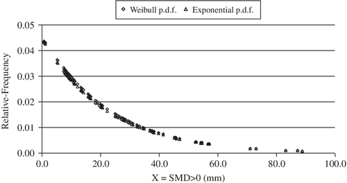
A comparison between the estimated exponential PDF (12) with that of weibull density (11) is shown in Figure 4, which confirms a close agreement between the two density functions.

5 THRESHOLD SOIL MOISTURE DEFICIT

Values of the threshold soil moisture deficit (TSM) are achievable target SMD levels computed to increase the harvested crop-yield (potato in this study) close to a specified proportion of the maximum possible yield in the region; this may require additional water supply. To find an empirical relationship between SMD and evapotranspiration, Sx = Pw × RF, where RF, the rainfall (mm/month) is defined as the proportion of rainfall depleted at the rate of maximum evapotranspiration, Em. It is expected that [Ea/Em] would decrease with the increase of [SMD/Sx] and vice versa, that is, a negative correlation between them. A linear relationship between these two variables is shown below.

[SMD / Sx] = ω_{1} + ω_{2} [Ea / Em],

(13)

where, the regression constant, ω₁ = 33.15, regression coefficient ω₂ = − 32.78, and R² = 51%. Estimated Equation (13) is shown in Figure 5 by a solid straight line. A reasonable maximum value of [SMD/Sx] corresponding to the minimum [Ea/Em] and a minimum value of [SMD/Sx] corresponding to the maximum [Ea/Em] are identified by shifting the line (13) downward by changing values of ω₁ and ω₂ through “trial and error”. Initial threshold values of TSM are estimated by replacing values of ω₁ and ω₂ in (13) by their new values, ω₃ = 16.808 and ω₄ = − 16.214 respectively as shown below and by a broken line in Figure 5.

TSM = Sx (ω_{3} + ω_{4} [Ea / Em]),

(14)

where, ω₃ = 16.808 and ω₄ = − 16.214.

The min[TSM] = 2.12 and max[TSM] = 74.52 are estimated incorporating the max[Ea/Em] = 1.0 and min[Ea/Em] = 0.484, respectively in Equation (14). Other initial values of TSM are also computed repeating the above procedure. The above approach although tentative, provides a workable means for computing the initial TSM values. The effect of water stress in the plant and yield loss is generally measured by the following linear equation7, 61:

ky [1 - (Ea / Em)] = [1 - (Ya / Ym)],

(15)

where, Ya and Ym respectively are the actual and maximum harvested yield (tons/ha), ky = 1.12, the yield response factor of crop (potato) over the growing season.7 To increase the harvested yield (potato) close to a specified proportion of the maximum yield, a target 95 % = (Ya/Ym) is set and substituted in Equation (15) to estimate a fixed [Ea/Em] as follows:

[Ea / Em] = 1 - [1 / 1.12] \times [1 - .95] = 0.9554 \approx 0.96 .

Thus, the initial TSM values approximately ensuring a relative yield close to 95% is given by:

Y = TSM = Sx \times (ω_{3} + ω_{4} [Ea / Em]),

(16)

where, [Ea/Em] ≈ 0.96, ω₃ = 16.808 and ω₄ = − 16.214.

The Kolmogorov-Smirnov goodness of fit test (K-S test) confirmed at the 95% level that the PDF of initial TSM (Y) could be approximated by an exponential distribution. The initial estimates of Y from Equation (16) are compared with the data, generated from an exponential distribution with the mean of initial Y values, which is 17.21 mm. Figure 6 shows that a few points at the upper end needs adjustment. Finally, the estimated Y values are adjusted and the PDF of adjusted TSM, Y is estimated as follows:

f_{Y} (y) = a_{2} \exp (- a_{2} y), y > 0 .

(17)

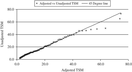
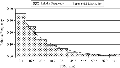
For the PDF (17), the rate parameter, a2 = 0.0575 and the mean, 1/a2 = 17.388.

A comparison between the frequency distribution of TSM data and its approximation by the exponential distribution (17) is reasonable as shown in Figure 7.

6 PROBABILITY DISTRIBUTION OF (SMD-TSM)

The variable (SMD-TSM) is a mixture of two independent variables. They are (SMD − TSM) > 0, the subnormal state and SMD-TSM) ≤ 0, the normal state of the CGP, which follows from the definition of drought in Section 2.1 and Figure 2. Thus the PDF of (SMD-TSM) is a mixture of two independent probability distributions; the PDF of (SMD − TSM) > 0, and the PDF of SMD-TSM) ≤ 0. The PDF of SMD = X is f_x(x) = a₁exp(−a₁x) for x > 0 and that of TSM = Y is f_y(y) = a₂exp(−a₂y) for y > 0 from Equations 12-17 respectively. By independence the joint PDF of X and Y is

a_{1} a_{2} \exp (- a_{1} x) \times \exp (- a_{2} y), x, y > 0 .

(18)

Let R = (X − Y). The intention is to find the probability distribution of R from the joint distribution (18). Consider R = r is fixed. When R > 0, implies the CGP is in subnormal state and for R ≤ 0 the CGP in normal state. We first formulate the cumulative distribution function (CDF), F_R(r), that is, Pr(R < r) = Pr(X − Y < r) then differentiate F_R(r) to get the PDF, f_R(r). From Equation (18) it appears that the PDF, f_R(r) of R will occur in pair, where the pair is separated at r = 0. We first consider the Case 1, when r ≤ 0 and then Case 2, when r > 0.

Case 1.r ≤ 0.

\begin{align} F_{R} (r) = \Pr (R \leq r) & = \Pr (X - Y \leq r) \\ = \Pr (Y \geq X - r) \\ = \int_{0}^{\infty} a_{1} \exp (- a_{1} x) [\int_{x - r}^{\infty} a_{2} \exp (- a_{2} y) dy] dx [From (18)] \\ = \int_{0}^{\infty} [a_{1} \exp (- a_{1} x) \exp (a_{2} r) \exp (- a_{2} x)] dx \\ F_{R} (r) & = \Pr (R \leq r) = [a_{1} / (a_{1} + a_{2})] \exp (a_{2} r) . \end{align}

Differentiating the above CDF, the PDF, f_R(r) for r ≤ 0 is

f_{R} (r) = [a_{1} / (a_{1} + a_{2})] a_{2} \exp (a_{2} r), r \leq 0

(19)

Case 2.r > 0.

\begin{array}{l} F_{R} (r) & = \Pr (R < r) = \Pr (X - Y < r) \\ = 1 - \Pr (X - Y > r) \\ = 1 - \Pr (Y < X - r), since r > 0 \\ = 1 - \int_{r}^{\infty} a_{1} \exp (- a_{1} x) [\int_{0}^{x - r} a_{2} \exp (- a_{2} y) dy] dx [From (18)] \\ = 1 - \exp (a_{2} r) \int_{r}^{\infty} a_{1} \exp - (a_{1} + a_{2}) x dx - \int_{r}^{\infty} a_{1} \exp (- a_{1} x)] dx \\ = 1 + [a_{1} \exp (a_{2} r) / - (a_{1} + a_{2})] - \exp (a_{1} r) \\ F_{R} (r) & = \Pr (R < r) = 1 - [a_{2} / (a_{1} + a_{2})] \exp (- a_{1} r) . \end{array}

Differentiating the above CDF., the PDF, f_R(r) for r > 0 is

f_{R} (r) = [a_{2} / (a_{1} + a_{2})] a_{1} \exp (- a_{1} r), for r > 0 .

(20)

From Equations 19-20, the PDF of r is.

\begin{array}{l} \{[a_{1} / (a_{1} + a_{2})] a_{2} \exp (a_{2} r), for r \leq 0 \\ f_{R} (r) = \\ \{\{[a_{2} / (a_{1} + a_{2})] a_{1} \exp (- a_{1} r), for r > 0 . \end{array}

(21)

This is an asymmetric Laplace distribution with parameters a₁ and a_2.62 The PDF (21) is rescaled introducing the asymmetric parameter Sk to express a1 and a2 (rate parameters of f_x(x) and f_y(y) respectively) in terms of the rate parameters of r > 0 and r ≤ 0 in Equation (21) as follows. From Kozubowski and Podgorski,63 we have

Sk = (2 / γ) / (m_{1} + {[(4 / γ^{2}) + {(m_{1})}^{2}]}^{1 / 2}), where

$m_{1} = \sum_{i = 1}^{n} R_{i} / n = 4.969 is the mean of R = (X - Y) and n = 120, the sample size .$

Since the scale parameter γ of r is unknown, the maximum likelihood estimate of γ is computed from the sample as62:

$1 / γ = \sum_{i = 1}^{n} |R_{i}| / n = \sum_{i = 1}^{n} |X_{i} - Y_{i}| / n = 22.798, γ = 0.0439, n = 120 .$

The estimate of Sk = 0.8969 from the above formula for Sk.

Substituting a1 = γ Sk and a2 = γ/Sk, the PDF (21) becomes.

\begin{align} \{[{Sk}^{2} / (1 + {Sk}^{2})] [(γ / Sk) \exp[(γ / Sk) r] = f_{R} (r_{(-)}), for r \leq 0 \\ f_{R} (r) = { \\ \{[1 / (1 + {Sk}^{2})] (γ Sk) \exp - [(γ Sk) r] = f_{R} (r (+)), for r > 0 . \end{align}

(22)

Writing r₊ for r > 0 and r₋ for r ≤ 0, the proportion of the area of PDF, f_R(r₍₊₎) is 1/(1 + Sk²) = 0.554 as shown by the right hand side of Figure 8. Similarly, the proportion of the area of PDF, f_R(r₍₋₎) is Sk²/(1 + Sk²) = 0.446, the left hand side of Figure 8, such that f_R(r) = f_R(r₍₋₎) + f_R(r₍₊₎) = 1 is the total area of PDF, f_R(r) in Figure 8. Figure 8 shows that subnormal state of the CGP is likely to occur marginally more frequently than the normal state in East Anglia. The above proportions of area for f_R(r₍₊₎) and f_R(r₍₋₎) respectively are not significantly different from the estimates, a₂/(a₁ + a₂) = 0.563 for r > 0 and a₁/(a₁ + a₂) = 0.438 for r ≤ 0 as shown by Equation (21). This indicates, rewriting 21-22 by introducing Sk does not change properties of the original f_R(r) in Equation (21). The PDF f_R(r), in Equation (22) is an alternate form of Equation (21) with γ₁ = γSk = 0.03934 and γ₂ = γ/Sk = 0.04894, the scale parameters for f_R(r₍₊₎) and f_R(r₍₋₎), respectively. The parameter, Sk simply measures the extent of asymmetry between the PDF f(r₍₊₎) (subnormal state of the CGP) and the PDF f(r₍₋₎) (normal state of the CGP) measured by (SMD-TSM). The asymmetric Laplace distribution (22) is a mixture of a positive and a negative exponential distributions, since f_R(r) in Equation (22) can be written as64:

f_{R} (r) = [1 / (1 + {Sk}^{2})] f_{R} (r_{(+)}) + [{Sk}^{2} / (1 + {Sk}^{2})] f_{R} (r_{(-)}) .

(23)

Thus the PDF of r₍₊₎ is f_R(r₍₊₎) = γ₁exp(−γ₁r₍₊₎) and that of r₍₋₎ is f_R(r₍₋₎) = γ₂exp(γ₂ r₍₋₎), where γ₁ = (γ Sk) and γ₂ = (γ/Sk). This study requires the PDF of (SMD − TSM) > 0, that is, the PDF of r₍₊₎ to estimate of the PDF of run-sum defined in Section 7. From Equation (23), the PDF, f_R(r₍₊₎) for r₍₊₎ is given by:

f_{R} (r_{(+)}) = γ_{1} \exp (- γ_{1} r_{(+)}), r_{(+)} > 0 .

(24)

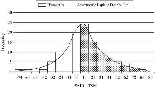
Estimates of the rate parameter, γ₁ = 0.03934 and the mean of r₍₊₎ (the positive SMD-TSM values) is 1/γ₁ = 25.419 mm in East Anglia.

7 AGRICULTURAL DROUGHT COMPONENTS

The variables, run-length (T), WSP-sum (W), and run-sum (Z) for agricultural drought are defined as follows:

Suppose,

T = t_{i,} i = 1, 2, 3 \dots m,

(25)

where, T is the number of consecutive monthly SMD (mm) greater than monthly TSM (mm), preceded and followed by a SMD less than or equal to a TSM for the ith dry period/drought event; Equation (25) defines the run-length or the duration T (months) of the ith event and m is the total number of dry period/drought events. The WSP-sum, W (in mm) is defined as the total amount of WSP given by (Em_j-Ea_j) >0 over t_i consecutive months for the ith drought.

W = \sum_{j = 1}^{t_{i}} ({Em}_{j} - {Ea}_{j}), {Em}_{j} > {Ea}_{j},

(26)

where, Em_j and Ea_j are the maximum and actual evapotranspiration respectively in month j during the ith drought event of duration t_i (months).

The run-sum, Z (in mm) over the duration t_i of the ith drought is

Z = \sum_{j = 1}^{t_{i}} (X_{j} - Y_{j}) = \sum_{j = 1}^{t_{i}} r_{(+) j}, X > Y, r_{(+)} > 0 .

(27)

8 PROBABILITY DISTRIBUTIONS OF RUN-LENGTH AND RUN-SUM

8.1 Probability distribution of run-length

Methods for the derivation of the probability distribution of Run-length (T) are discussed in Section 2.2.1. The probability mass function (p.m.f.) of run-length, T = t, a discrete random variable (r.v.) has geometric distribution with the mean 1/p,15 where p is the probability of normal state and q = 1 − p, the probability of subnormal state of the CGP and the distribution is.

\Pr (T = t) = p q^{t - 1}, n = 1, 2, 3, \dots

(28)

If T = t is a continuous and differentiable r.v., the PDF of T is the exponential distribution as follows.9

f_{1} (t) = λ_{1} \exp (- λ_{1} t), t > 0 .

(29)

The scale parameter is λ₁ = p and the mean, 1/λ₁ = θ/p = 1/p, since the interval between t_i and t_i + 1 is θ =1 (month) in this study. Two alternate distributions 28-29 of run-length follows from the unique property of the exponential and geometric distributions discussed in Section 2.2.1.9, 26 The MLE of parameters for (28) are P = 0.4225 and the mean 1/p = 2.367. The rate parameter for (29) is λ₁ = p = 0.4225 and the mean 1/λ₁ = 1/p = 2.37, since θ = 1.

8.2 Probability distribution of run-sum

The theorem, Sum of Random Number of Continuous Random Variables (r.v.) states the following9:

If R_(+)1,R_(+)2,R_(+)3,………R_(+)n_, are identically and independently distributed (i.i.d.) exponential r.v. with the common mean 1/γ₁, (ie, the PDF (24)) and that n = t_i, the total number of consecutive dry periods of the ith drought (run-length) and
the probability distribution of T_i is given by (28), a geometric distribution with the mean 1/p and that T_i is independent of R₍₊₎,

then the PDF of Z = R₍₊₎₁ + R₍₊₎₂ + R₍₊₎₃ + … + R_(+)n is given by:

f_{2} (z) = λ_{2} \exp (- λ_{2} z), z > 0 .

(30)

The MLE of the rate parameter λ₂ = pγ₁ = p(γSk) = 0.4225 × 0.03934 = 0.0166 and the mean 1/λ₂ = 60.16. It may be noted that 1/λ₂ = 54.497 ≈ 54.5 estimated from observed run-sum is marginally lower due to approximate value of γ in Equation (22). For the same reason λ₂ = 0.0183, estimated from the sample is marginally higher than λ₂ = 0.0166.

9 PROBABILITY DISTRIBUTION OF WSP-SUM AND FAILURE RATE FUNCTION

9.1 Probability distribution of WSP-sum

The increase of crop-water stress, WSP-sum (W) with increase of run-length (T), the duration and run-sum (Z), the severity during drought is discussed in Section 2.1. The dependence of W on T and Z is given by the crop-water Stress function (as in Section 2.1) as follows:

w = B 1 . t + B 2 . z, w, y, z > 0,

(31)

where, w, t, z are variate values of W, T and Z and B1, B2 are constants, such that B1, B2 > 0 and B1 ≠ B2. The coefficient, B1 measures the change in WSP-sum, W per unit change in run-length, T and B2, measures the same for run-sum, Z. The Stress function (31) measures the subnormal state of CGP as the total WSP-sum, W during a drought; where the WSP-sum is defined in Equation (31) as the sum of two components, (a) the run-length component (B1.t), and (b) the run-sum component (B2.z). For the derivation of the PDF of W, the run-length is assumed as a continuous random variable and the marginal PDF of run-length is exponential on the basis of the unique property as in Section 2.2.1 and Section 8.1. Under independence, the PDF of W is derived from the joint PDF of run-length, T in Equation (29) and run-sum, Z in Equation (30) as follows:

\begin{align} g (w) & = f_{1} (t) \times f_{2} (z), w, y, z > 0 \\ g (w) & = λ_{1} \exp {(- λ_{1} t)}^{*} λ_{2} \exp (- λ_{2} z) [From (29) and (30)] . \end{align}

(32)

\begin{matrix} Let B 1 t & = u implies t = (1 / B 1) u = k_{1} u, where, 1 / B 1 = k_{1}, u > 0 and \\ B 2 z & = v implies z = (1 / B 2) v = k_{2} v, where, 1 / B 2 = k_{2}, v > 0, \end{matrix}

where, g(w) is the PDF of W. Now, substituting u and v in Equation (31)

w = u + v, u > 0, v > 0 .

(33)

In (33), u = run-length component B1.t and v = run-sum component B2.z.

Substituting, t = k₁u and z = k₂v, one obtains from Equation (32)

\begin{align} g (w) & = λ_{1} k_{1} \exp {(- λ_{1} k_{1} u)}^{*} λ_{2} k_{2} \exp (- λ_{2} k_{2} v) du dv \\ = α_{1} \exp (- α_{1} u) du α_{2} \exp (- α_{2} v) dv, \end{align}

(34)

where, α₁ = λ₁k₁ and α₂ = λ₂k₂

From Equation (33), v = w – u, implying that 0 < w – u < ∞ and 0 < u < w, u, w > 0.

Thus, from Equation (34), we have

\begin{align} g (w) & = α_{1} \exp (- α_{1} u) du α_{2} (\exp - α_{2} (w - u)) dw \\ = α_{2} \exp (- α_{2} w) α_{1} \exp (- (α_{1} - α_{2}) u) du dw . \end{align}

Integrating u out gives.

\begin{align} g (w) & = α_{2} \exp (- α_{2} w) [\int_{0}^{w} α_{1} \exp (- (α_{1} - α_{2}) u) du] dw \\ = α_{2} \exp (- α_{2} w) [(α_{1} / (α_{1} - α_{2})) - (α_{1} / (α_{1} - α_{2})) \exp (- (α_{1} - α_{2}) w)] dw \end{align}

Thus, the PDF, g(w) of WSP-sum (W) is

g (w) = [α_{1} α_{2} / (α_{1} - α_{2})] [\exp (- α_{2} w) - \exp (- (α_{1} w)], w > 0, α_{1} \neq α_{2} .

(35)

Alternately, Equation (35) can be presented as:

g (w) = A 1 [α_{2} \exp (- α_{2} w)] + A 2 [α_{1} \exp (- (α_{1} w)], w > 0, α_{1} \neq α_{2} .

(36)

Equations 35-36 are the same hypoexponential distribution [hypo∼(α₁, α₂, w)] in two alternate forms with parameters α₁ and α₂.9, 65, 66 The PDF g(w) of WSP-sum (W) defines the subnormal state of CGP as a sum of two independent exponentially distributed sequential phases; Phase-1 influenced by the average run-length and Phase-2 influenced by the average run-sum. The PDF, g(w) therefore divides the failure probability of WSP-sum estimated from Equation 35-36 into two phases, representing the likelihood of the overall subnormal state (failure) of CGP to occur during drought.

The density function g(w), Equation (35) appears in Equation (36) as a weighted sum of two exponential density functions in two phases into a series, though one of the weights can be negative. The weights in Equation (36) are A1 = α₁/(α₁ − α₂) and A2 = α₂/(α₂ − α₁) such that A1 + A2 = 1. The notion of “sum” does not mean “arithmetic sum” but a “mixture” of two subpopulations (Phases-1 and 2), each of which is exponentially distributed with the rate parameters α₁ and α₂, respectively.9 The physical interpretation of α₁ and α₂ may be given as follows:

From Equation (34), α₁ = λ₁k₁ = 1/[(1/λ₁) × B1)], where λ₁= rate parameter of the PDF of run-length and 1/λ₁= mean of rum-length as in Equation (29) and 1/k₁ = B1, the WSP-sum per unit run-length. Similarly, α₂ = λ₂k₂ = 1/[(1/λ₂) × B2)], where λ₂ = rate parameter of the PDF of run-sum and 1/λ₂ = mean of rum-sum as in Equation (30) and 1/k₂ = B2, the WSP-sum per unit run-sum as defined in Equation (31). Substituting 1/λ₁ and 1/λ₂ in Equation (31) the mean WSP-sum to failure, μ per drought event is:

\begin{align} μ & = B 1 \times (1 / λ_{1}) + B 2 \times (1 / λ_{2}) \\ = [(WSP - sum per unit run - length) \times (mean of rum - length) + \\ (WSP - sum per unit run - sum) \times (mean of rum - sum)] \\ = (mean of Phase - 1) + (mean of Phase - 2) \\ = (1 / α_{1}) + (1 / α_{2}) . \end{align}

It can be shown that the variance of WSP-sum, σ² = 1/(α₁)² + 1/(α₂)² and the coefficient of variation, (c. v.) = σ/μ. The estimated mean (μ) and variance (σ²) of hypo∼(α₁, α₂, w) are combinations of the mean and variance of two independent exponential distributions of Phases-1 and 2.9

Integrating (35), the CDF G(w) of WSP-sum is given as follows:

Writing W * = [α₁α₂/(α₁ − α₂)]

\begin{align} G (w) & = W^{*} [\{(1 / α_{2}) - (1 / α_{2}) \exp (- α_{2} w)\} - \{(1 / α_{1}) - (1 / α_{1}) \exp (- α_{1} w)\}] \\ G (w) & = 1 - \{[1 / (α_{1} - α_{2})] [α_{1} \exp (- α_{2} w) - α_{2} \exp (- α_{1} w)]\} . \end{align}

(37)

Thus, the reliability or survival function R* of the CGP in terms of W is:

R^{*} = 1 - G (w)

(38)

9.2 Failure (or Hazard) rate function [h(w)]

The failure (or hazard) rate function h(w) of WSP-sum, W is as follows66:

h (w) = g (w) / (1 - F (w), where, F (w) = \Pr (W < w) .

(39)

From Equations 37-39 follows that

h (w) = α_{1} α_{2} [\exp (- α_{1} w) - \exp (- α_{2} w)] / [α_{2} \exp (- α_{1} w) - α_{1} \exp (- α_{2} w)] .

(40)

The failure rate function h(w) indicates the speed (or risk) at which the subnormal state of CGP occurs. It determines either a premature end of the CGP, which may occur due to wilting of the crop or a successful end of the CGP, if it survives until the end of cropping season. In other words h(w) describes the lifetime of CGP66 discussed further in Section 11.1.

10 EXPECTED DROUGHT COMPONENTS FOR SPECIFIED RETURN PERIODS

While return periods of observed droughts are estimated from the failure probabilities of the CGP from Equation (37), the following procedures estimate (the other way round), the expected run-sum, run-length and WSP-sum components of designed droughts for specified return periods. The expected WSP-sum,

{\hat{w}}_{(Rp)}

for specified return periods, Rp of agricultural droughts are estimated from the nonlinear Equation (37), which is solved by the Newton's iteration method as follows. Setting the failure probability, P_Rp = [1 − (1/Rp)], for a given return period Rp, the iteration process is:

w_{i} = w_{i - 1} + [G (w) / G^{/} (w)] - P_{Rp},

(41)

where, the CDF of WSP-sum (W) from Equation (37) is

G (w) = 1 - \{[1 / (α_{1} - α_{2})] \times [α_{1} \exp (- α_{2} w) - α_{2} \exp (- α_{1} w)]\} .

Differentiating G(w),

G^{/} (w) = [α_{1} α_{2} / (α_{1} - α_{2})] \times [\exp (- α_{2} w) - \exp (α_{1} w)] .

The iteration process (41) is continued until w_i = w_i − 1, denoted by

{\hat{w}}_{(Rp)}

. Denoting ŵ as the estimate of w from Equation (31), the proportion of WSP-sum explained by the run-length component, B1.t and run-sum component, B2.z are as follows:

1 = (B 1 t / \hat{w}) + (B 2 z / \hat{w}),

(42)

(B 2 z / \hat{w}) = 1 - (B 1 t / \hat{w}) .

(43)

Define (B1t/ŵ) as a linear function of

\hat{w}

as follows:

(B 1 t / \hat{w}) = g 1 + (g 2 / \hat{w}), R^{2} = 51 %,

(44)

where, the least square estimates of g1 = 0.471 and g2 = 4.334. Thus,

t = [g 1 + (g 2 / \hat{w})] \times [\hat{w} / B 1] .

(45)

From Equations (43) and 44)

z = [1 - (g 1 + (g 2 / \hat{w})] \times[\hat{w} / B 2] .

(46)

Suppose,

{\hat{w}}_{(Rp)}

is a fixed WSP-sum for a specified return period Rp estimated from Equation (41). The corresponding estimate of run-length

{\dot{t}}_{(Rp)}

, which is unknown, can be computed from Equation (45) as follows.

{\dot{t}}_{(Rp)} = [g 1 + (g 2 / {\hat{w}}_{(Rp)})] \times [{\hat{w}}_{(Rp} / B 1] .

(47)

Similarly, the estimate of run-sum, Z_(Rp) (which is unknown) corresponding to ŵ_(Rp) can be computed from Equation (46) as follows.

{\hat{z}}_{(Rp)} = [1 - (g 1 + (g 2 / {\hat{w}}_{(Rp)})] \times[{\hat{w}}_{(Rp)} / B 2] .

(48)

The expected values ${\hat{w}}_{(Rp}$ and ${\hat{z}}_{(Rp)}$ are water stress in the plant and severity (run-sum,) respectively over the expected duration ${\dot{t}}_{(Rp)}$ (run-length,) of agricultural drought for the specified return period of Rp.

11 RESULTS AND CONCLUSIONS

11.1 Results and discussions

Proportions of soil-water depletion (Pw) at the rate of daily maximum evapotranspiration (em) for the crop (potato), discussed in Section 3 is estimated from the data available from Doorenbos and Kassam7 as follows:

Pw = β1 \times {em}^{β2}, β1 = 2.35, β2 = 0.508, R^{2} = 98.6 % .

Substituting the observed em values in the above equation the corresponding Pw values are computed. The monthly effective rainfall (IP) and the corresponding total rainfall (RF) data are available from the FAO study on the irrigation and water management.8 A statistical relationship between IP and RF (>20 mm) is defined using the FAO data as follows:

IP = a + b {RF}_{,} R^{2} = 99.7 %, where, a = - 13.773, b = 0.6864 .

The observed monthly rainfall data of East Anglia are substituted in the above formula to estimate the corresponding IP for the estimation of SMD as in Section 3.

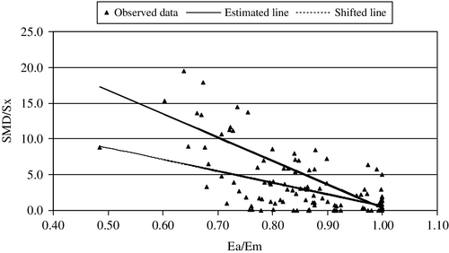
Monthly soil moisture deficit (SMD), the maximum and actual evapotranspiration (Em and Ea, respectively) are computed as in Section 3. PDFs of SMD, threshold SMD (TSM) and (SMD-TSM) and their parameters are discussed in Sections 4-6, respectively. Density functions of run-length and run-sums and their parameters are presented in Section 8. The WSP-sum (W) and run-sum (Z) over the duration (T) of drought as discussed in Section 7 are shown in Figure 9.

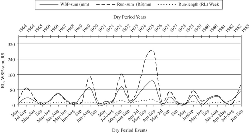
The agricultural activities in East Anglia extend from April-September (6 months) followed by the winter; the maximum drought duration (run-length) of 6 months is considered in this study.

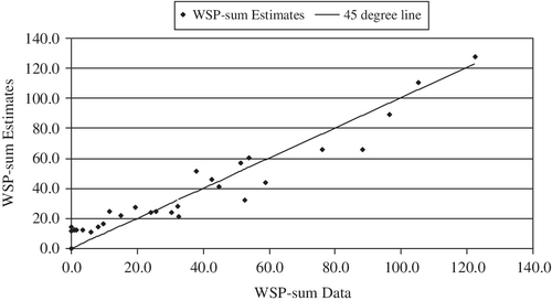
The increase of WSP-sum (W) with increase of run-length (T) and run-sum (Z) as in Figure 9 provides a reasonable evidence of positive correlation of WSP-sum with run-length (88.3%) and run-sum (84.3%). The estimated Stress function (31) defines a linear relationship of (W) with (T) and (Z) as in Figure 10. The coefficient, B1 = 9.9211 in Equation (31) indicates the increase of WSP-sum (W in mm) for unit increase of the run-length (T in month). The coefficient, B2 = 0.2449 in Equation (31) measures the same for run-sum (Z in mm). The Stress function (31) explains over 96% of variations of the water stress in the plants (W) due to run-length (duration T) and run-sum (severity Z) during dry periods in East Anglia. Figure 10 also shows the degree of closeness between the observed and estimated WSP-sum relative to the 45° line.

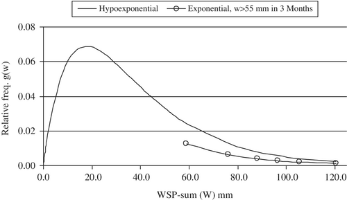
The PDF of W, given by g(w) is a [hypo∼(α₁, α₂, w)] derived from the Stress function (31) and the joint distribution of T and Z as shown in Figure 11. Figure 11 shows that g(w) is a long tailed distribution, skewed to the right, which generally characterizes such rare events as droughts and floods in hydrological studies. The PDF g(w) consists of two independent exponentially distributed phases, Phases-1 and 2 as in Equations 35-36 discussed in Section 9.1. Estimated parameters of g(w) are α₁ = 0.0412 and α₂ = 0.0749, A1 = α₁/(α₁ − α₂) = − 1.219 and A2 = α₂/(α₂ − α₁) = 2.219 such that A1 + A2 = 1. For the PDF g(w) from Section 9.1, the estimated mean, μ = 37.612, variance, σ² = 768.069, SD, σ = 27.71 and the coefficient of variation, c.v. = 0.74 (which is <1). The PDF g(w) is a hypo∼(α₁, α₂, w), since the coefficient of variation, c.v. < 1 (,9 p. 29). The mode of WSP-sum occurs in between 10 and 20 mm in East Anglia (Figure 11).

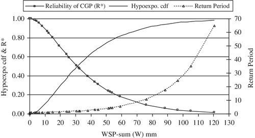
The CDF G(W) (37) and reliability R* (38) of the PDF g(w) as in Figure 12 show that the chance of survival (reliability) of the CGP (measured by the WSP-sum, W) gradually decreases with the increase of failure probability. The point of intersection between the CDF and the reliability function, where WSP-sum = 30 mm and a 50% chance for the CGP to be in subnormal state in East Anglia. Figure 12 also shows, the reliability of CGP starts decreasing exponentially for the WSP-sum greater than 40 mm and the failure probability is about 60%. A summary of Figure 12 presented in Table 1 contains the average values of crop-water stress, (WSP-sum), severity (run-sum) over droughts durations (run-length) ranging from 1 to 6 months. Table 1 also shows the failure and survival probabilities (reliability) and estimated return periods of observed drought events. As in Table 1, there are 17 out of 29 drought events have duration 1 or 2 months in East Anglia. The Crop-water stress and run-sum are not very high; the probability of survival for the CGP stays between 98% down to 64%. September, the likely dry month for these events is really the harvesting period, when the water supply ceases to exist. The extreme dry months in East Anglia are June, July and August. During these months, about 20% of drought events have duration, 3 months and return period, 6 years; the severity (run-sum) is about 80 mm, crop-water stress, 54 mm and reliability of the CGP is 84%.

Table 1. Dry period frequency, averages of WSP-sum, run-sum, failure probability, reliability and return periods for run-length 1 to 6 months

(1)	(2)	(3)	(4)	(5)	(6)	(7)	(8)
Run-length	Dry period frequency	Average WSP-sum	Average run-sum	Failure prob. of WSP-sum	Reliability of WSP-sum	Return period of drought (Year)	Likely dry period months
1	9	4.0	12.7	0.032	0.968	1	May; Sep
2	8	24.0	19.8	0.361	0.639	2	May-Jun; Jul-Aug
3	6	54.1	79.1	0.836	0.164	6	Jun-Aug; Jul-Sep
4	3	81.5	114.1	0.914	0.086	12	Jun-Sep; Apr-Jul
5	2	101.0	204.1	0.966	0.034	30	May-Sep
6	1	120.5	278.4	0.985	0.015	65	Apr-Sep
Total events	29

Note: (1) Run-length (RL): Duration of dry period/drought event. (2) Drought frequency: Number of dry period/drought events. (3) Average WSP-sum: Average Crop-water Stress. (4) Average Run-sum (RS): Average severity (RS) of drought. (5) Failure Prob. of WSP-sum: Failure probability of WSP-sum. (6) Reliability of WSP-sum: Survival probability of WSP-sum. (7) R.P. of drought: Average Return Period (R.P.) of WSP-sum. (8) Dry period months: Likely dry period months for WSP-sum ≥40 mm.

A drought event with duration greater than or equal to 3 months is a warning sign for the WSP-sum, which may become greater than 40 mm in East Anglia. There are only 6 drought events (out of 29), which have durations in the range of 4 to 6 months and return periods 12 to 65 years, indicating a very low reliability of the CGP between 8.6% down to 1.5%. During these drought events the cumulative water-stress in the plant (WSP-sum) could be as high as 81 mm to 121 mm and run-sum 114 mm to 248 mm. The drought of 6 months duration (or higher) occurred in 1975/76 was one of the most severe drought in the recent years in England and Wales. In general, Table 1 indicates that dry periods/droughts are seasonal phenomena in East Anglia.

When agricultural drought gradually approaches a very high severity and longer duration, the PDF g(w), (35) tends to the exp∼(α_k, w) with the rate parameter α_k, where, α_k = min{α₁, α₂}, α₁ = 0.0412 and α₂ = 0.0749 are the failure rate parameters of PDF g(w) (35). In other words, PDF g(w), a hypo∼(α₁, α₂, w) becomes exp∼(α₁, w), since α_k = α₁ = 0.0412. This can be proved multiplying the numerator and denominator of (40) by exp(−α₁w); as w → ∞, h(w) = α₁ = 0.0412 = α_k. Figure 11 shows a comparison of the exponential PDF α₁exp(−α₁w) (shown by circles) with the lower part of hypo∼(α₁, α₂, w). The PDF α₁exp(−α₁w) with the failure rate parameter α_k = α₁ = 0.0412 (similar to Equation (12a) in Section 4) defines the lifetime of the CGP as in Figure 13.

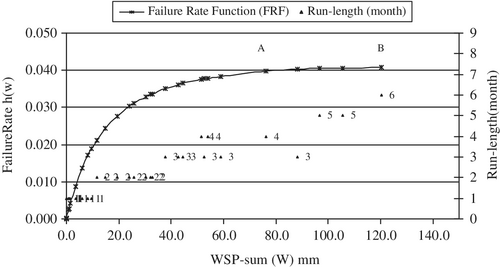
The gradual rise of the failure (or hazard) rate function to α_k is generally very sharp (or faster) for events like the mechanical device failure due to their nature of sudden occurrence and their estimated lifetime is given with respect to time. But for drought the process is very slow due to the occurrence of drought is creeping in nature and gradually becomes severe with the increase of run-length (T) and run-sum (Z) and WSP-sum (W). A section of the failure rate function, h(w), starting approximately at the point A and ending at B is almost a straight line as in Figure 13. The line A to B represents the failure rate function α_k = α₁ = 0.0412 (constant, similar to Equation (12a) in Section 4) and the distribution, α₁exp(−α₁w) defines the lifetime of the CGP, provided it survives beyond the point A.

Figure 13 shows for α_k = α₁ = 0.0412 and the corresponding WSP-sum is somewhere between 105.4 and 120.5 mm over run-lengths 5 (April to August) and 6 months (April to September) respectively and the monthly average WSP-sum is about 21 mm computed from 105.4/5 and 120.5/6, which is not significantly high. At this stage, the CGP is less likely to survive unless there is additional water supply or it is the harvesting time, that is, the end of CGP. Figure 13 indicates that the CGP somehow survived nearly the end of the crop growing session but may not be up to its full potential. In East Anglia, June, July and August are the driest months (see Figure 9), when the crop water demand is high. If the failure rate function, h(w) reaches α_k (=α₁) long before the harvesting period then the stolonization, tuber initiation followed by yield formation would be in a critical state. As a result wilting of the crop or yield reduction would occur unless the required irrigation or rainfall is available.

While Figure 12 shows estimated return periods of observed droughts, Figure 14 shows the other way round, that is, a profile of designed droughts depicted by their expected run-sum (Z_(Rp)), run-length (t_Rp)) and WSP-sum (ŵ_(Rp)) estimated from 41-48 respectively for specified return periods of 5 years and then 10 to 100 years at a 10 years interval as in Section 10.

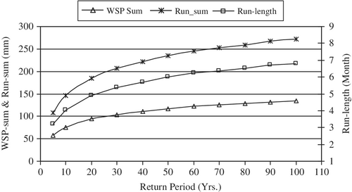
In East Anglia, the longest return period of drought is just about 65 years as evidenced by the drought in 1975/1976 (Figure 12), which was a severe drought relative to the climate in England and Wales. For a 60 years return period, the expected WSP-sum is about 120 mm and the corresponding run-length, about 6 months and rum-sum, 245 mm as in Figure 14.These values of WSP-sum, run-length and run-sum are very close to those in Table 1 for a 65 years return period. The expected drought components for return periods greater than 65 years as in Figure 14 are less likely to occur in England and Wales. The designed drought run-sums are the expected amount of soil-water loss due to droughts (opportunity loss), which could have been used for potato production had the period been a normal year. The above information and the others would be useful for proactive water resources planning to mitigate the impact of droughts.

11.2 Conclusions and recommendations

The study establishes that the Crop Growing Process (CGP) is very similar to the functioning of a mechanical device and its components subject to failure. The subnormal state (or failure) of the CGP in East Anglia is in general a seasonal phenomenon with the average drought duration of about 2.37 months. The WSP-sum greater than 40 mm and drought duration of 3 months or greater is a warning sign of critical soil moisture shortage for the crop. The failure rate function, h(w) rises slowly due to creeping nature of drought occurrence measures the speed (or risk) of the failure and the lifetime of CGP. Return periods of severe droughts in East Anglia are less likely to exceed 70 years or so. The study suggests that the probabilistic characterizations of agricultural drought could be well depicted by the:

run-length, run-sum and WSP-sum, the failure rate function (Figure 13) and failure probabilities of the subnormal CGP and return periods (Figure 12 and Table 1) of observed droughts as well as
expected run-length, run-sum and WSP-sum estimated from designed droughts for a set of specified return periods (Figure 14).

In general, the combined influence of all the drought components upon the WSP-sum probabilistically characterizes agricultural drought, given the CGP. There is a scope for improving the TSM estimation procedure. A generalization of this study considering the weibull distribution is a topic recommended for future research.

ACKNOWLEDGEMENTS

The author is grateful to the anonymous reviewers for their very thoughtful and constructive comments and suggestions. Most of the data provided by the Anglian Water Authority and Meteorology Department, U.K. are thankfully acknowledged. Thanks are due to East Anglia University, Environment Science Department for providing the information on land use for agriculture and water supply in East Anglia region. Thanks are also due to Dr Amit Banerjee for proofreading the paper and Dr Alex Miller for his helpful suggestions in deriving the Asymmetric Laplace Distribution.

CONFLICT OF INTEREST

The authors have no conflict of interest relevant to this article.

REFERENCES

1 Cumani M, Rojas O. Characterization of the Agricultural Drought Prone Areas on a Global Scale: Using the FAO Agricultural Stress Index System (ASIS) to Enhance the Understanding of, and Boost Resilience to, Water Stress Conditions in Drought-Prone Areas. Rome, Italy: FAO; 2016.
Google Scholar
2Luo L, Apps D, Arcand S, Xu H, Pan M, Hoerling M. Contribution of temperature and precipitation anomalies to the California drought during 2012–2015. Geophys Res Lett. 2017; 44: 3184-3192.
10.1002/2016GL072027
Web of Science® Google Scholar
3Hao Z, Vijay P, Singh VP, Xia Y. Seasonal drought prediction: advances, challenges, and future prospects. Rev Geophy. 2018; 56(1): 108-141.
10.1002/2016RG000549
Web of Science® Google Scholar
4Mishra AK, Singh VP. A review of drought concept. J Hydrol. 2010; 403(1–2): 202-216.
10.1016/j.jhydrol.2010.07.012
Web of Science® Google Scholar
5Aboukhaled A. In: A Arar, AM Balba, BG Bishay, et al., eds. Research on Crop Water Use, Salt Affected Soils and Drainage in the Arab Republic of Egypt. Cairo, Egypt: FAO, The United Nations, Near East Regional Office; 1975.
Google Scholar
6Ramdas M, Govindaraju RS. Probabilistic assessment of agricultural droughts using graphical models. J Hydrol. 2015; 526: 151-163.
10.1016/j.jhydrol.2014.09.026
Web of Science® Google Scholar
7Doorenbos J, Kassam AH. Yield response to water. In: CLM Bentvelsen, V Brancheid, JMGA Plusje, M Smith, GO Uttenbogaard, HK Van der wal, eds. Food and Agric. Rome, Italy: Organisation of the United Nations; 1979: 33.
Google Scholar
8Brouwer C, Heibolem M. Irrigation and water management: irrigation water needs. Training Manual no. 3. Rome, Italy: FAO, UNO; 1986.
Google Scholar
9Medhi J. Stochastic Processes. 3rd ed. New Delhi, India: New Age Inter. Publishers; 2009.
Google Scholar
10Lockyer K, Muhlelman A, Oakland J. Production and Operations Management. 5th ed. London, UK: Pitman Publishing; 1988.
Google Scholar
11Epstein, B. The Exponential Distribution and its Role in Life Testing”. Technical Report No, 2, Dept. of Mathematics, Wayne State Univ., Michigan; 1958.
Google Scholar
12 Potopova V, Boroneant C, Boincean B, Souku J. Impact of agricultural drought on main crop yields in the Republic of Moldova. Int. J. Climatol. 2015; 36(4): 2063-2082. https://doi.org/10.1002/joc.4481.
10.1002/joc.4481
Web of Science® Google Scholar
13Sellam V, Poovammal E, Periasamy P. Estimating the impact of drought on crop yield using principal component analysis. J Web Eng. 2018; 17(6): 1980-1992.
Google Scholar
14Mishra AK, Singh VP. Drought modelling—a review. J Hydrol. 2011; 391(1–2): 157-175.
10.1016/j.jhydrol.2011.03.049
Web of Science® Google Scholar
15Kottegoda NT. Stochastic Water Resources Technology. London, UK: The Macmillan Press Ltd.; 1980.
10.1007/978-1-349-03467-3
Web of Science® Google Scholar
16Sharma A, Turboton DG, Lall U. Streamflow simulation: a nonparametric approach. Water Resor Res. 1997; 33(2): 291-308.
10.1029/96WR02839
Web of Science® Google Scholar
17Yevjevich V. An objective approach to definitions and investigations of continental hydrologic droughts. Hydrology Paper No. 23. Fort Collins, Colorado: Colorado State University; 1967.
Google Scholar
18Shiau JT, Shen HW. Recurrence analysis of hydrologic droughts of differing severity. J Water Resour Plann Manage. 2001; 127: 30-40.
10.1061/(ASCE)0733-9496(2001)127:1(30)
Web of Science® Google Scholar
19Dent D, Cook H. Performance of Agricultural Land. Norwich, UK: School of Environmental Sciences, University of East Anglia; 1986.
Google Scholar
20Dent D, Scammell RP. Assessment of long-term irrigation need by integration of data for soil and crop characteristics and climate. Soil Surv Land Eval. 1981; 1(3): 51-57.
Google Scholar
21Evans D. Agricultural demand for water in lowland areas. J Inst Water Eng Sci. 1983; 37: 513-521.
Google Scholar
22 Ansley J. On rocky ground-ALC System in England and Wales, Lichfields, England: Ministry of Agriculture, Fisheries and Food (MAFF); 2018. https//lichfields.uk/blog2018/december/4 onrocky-ground/. Accessed December 4, 2018.
Google Scholar
23Cancelliere A, Salas JD. Drought length properties for periodic stochastic hydrologic data. Water Resour. Res. 2004; 40: W02503. https://doi.org/10.1029/2002WR001750.
10.1029/2002WR001750
Web of Science® Google Scholar
24Gupta VK, Kisiel CC, Duckstein L. Droughts as extreme distribution from point rainfall process. Proceedings of the Second International Symposium in Hydrology. Fort Collins, Colorado: Water Resources Research Publications; 1973.
Google Scholar
25 White, N. (2015). Understanding Waiting Times Between Events with the Poisson and Exponential Distribution. https://nicolewhite.github.io/2015/05/23/understanding-waiting-times.html. Accessed May 23, 2015.
Google Scholar
26Prochaska BK. A note on the relationship between the geometric and exponential distributions. Am Stat. 1973; 27(1): 27.
Web of Science® Google Scholar
27Sen Z. Wet and dry periods of annual flow series. J. Hydrolic. Div., Proceedings of the ASCE. 1976; 35: HY10.
Google Scholar
28Sen Z. Run-sums of annual flow series. J Hydrol. 1977; 35: 311-324.
10.1016/0022-1694(77)90009-9
Web of Science® Google Scholar
29Chander S, Kambo NS, Spolia SK, Kumar A. Analysis of surplus and deficit using runs. J Hydrol. 1981; 49: 193-208.
10.1016/0022-1694(81)90212-2
Web of Science® Google Scholar
30Johnson NL, Kotz S. Distribution in Statistics: Continuous Multivariate Distributions. New York, NY: John Wiley & Sons; 1972.
Google Scholar
31Bonaccorso B, Cancelliere A, Rossi G. An analytical formulation of return period of drought severity. Stochastic Environ Res Risk Assessment. 2003; 17: 157-174.
10.1007/s00477-003-0127-7
Web of Science® Google Scholar
32Cancelliere A, Salas JD. Drought probabilities and return period for annual streamflow series. J Hydrol. 2010; 391: 77-89.
10.1016/j.jhydrol.2010.07.008
Web of Science® Google Scholar
33Mishra AK, Singh VP. Analysis of drought severity-area-frequency curves using a general circulation model scenario uncertainty. J Geophy Res. 2009; 114:D06120. https://doi.org/10.1029/2008JD010986.
10.1029/2008JD010986
Web of Science® Google Scholar
34Salas JD, Cancelliere A, Dustin D, Bode D, Pineda A, Vincent E. Characterising the severity and risk of drought in the Poudre River, Colorado. J Water Resour Plann Manage. 2005; 131(5): 383-393.
10.1061/(ASCE)0733-9496(2005)131:5(383)
Web of Science® Google Scholar
35Mukherjee D, Mansour N. A bivariate stochastic approach to estimate reliability of a pumped storage reservoir. J Hydrol. 1991; 125: 293-310.
10.1016/0022-1694(91)90034-F
Web of Science® Google Scholar
36Shiau JT. Fitting drought duration and severity with two-dimensional copulas. Water Resour Manage. 2006; 20: 795-815.
10.1007/s11269-005-9008-9
Web of Science® Google Scholar
37 Nelsen RB. An introduction to Copulas. New York, NY: Springer; 2006.
Google Scholar
38Reddy MJ, Ganguli P. Application of copulas for derivation of drought severity–duration–frequency curves. Hydrol Processes. 2012a; 26: 1672-1685.
10.1002/hyp.8287
Web of Science® Google Scholar
39Ganguli P, Ganguly A. Space-time trends in U.S. meteorological droughts. J. Hydrol. 2016; 8: 235-259.
10.1016/j.ejrh.2016.09.004
Web of Science® Google Scholar
40 Yan G, Tushar A, Ximing C. Spatial and temporal patterns of drought in the continental U.S. during the past century. Geophys Res Lett. 2016; 43: 6294-6303.
10.1002/2016GL069660
Web of Science® Google Scholar
41Tosunoğlu F, Onof C. Joint modelling of drought characteristics derived from historical and synthetic rainfalls: application of generalized linear models and copulas. J Hydrol. 2017; 14: 167-181.
10.1016/j.ejrh.2017.11.001
Web of Science® Google Scholar
42Ganguli P, Reddy MJ. Evaluation of trends and multivariate frequency analysis of droughts in three meteorological subdivisions of western India. Int J Climatol. 2014; 34: 911-928. https://doi.org/10.1002/joc.3742.
10.1002/joc.3742
Web of Science® Google Scholar
43DeMichele C, Salvadori G, Vezzoli R, Pecora S. Multivariate assessment of droughts: frequency analysis and dynamic return period. Water Resour Res. 2013; 49: 6985-6994.
10.1002/wrcr.20551
Web of Science® Google Scholar
44Song SB, Singh VP. Meta-elliptical copulas for drought frequency analysis of periodic hydrologic data. Stoch Environ Res Risk Assess. 2010; 24: 425-444.
10.1007/s00477-009-0331-1
Web of Science® Google Scholar
45Luetkemeier R, Stein L, Drees L, Liehr S. Blended drought index: integrated drought Hazard assessment in the Cuvelai-Basin. Climate. 2017; 5: 51.
10.3390/cli5030051
Web of Science® Google Scholar
46Samantaray AK, Gurjeet Singh G, Ramadas M, Panda RK. Drought hotspot analysis and risk assessment using probabilistic drought monitoring and severity–duration–frequency analysis. Hydrol Process. 2019; 33(3): 432-449. https://doi.org/10.1002/hyp.13337.
10.1002/hyp.13337
Web of Science® Google Scholar
47Alamgir M, Shahid S, Mohsenipour M, Ahmed K. Return periods of extreme meteorological droughts during monsoon in Bangladesh. Appl Mech Mater. 2015; 735: 186-189.
10.4028/www.scientific.net/AMM.735.186
Google Scholar
48Qutbudin I, Shiru MS, Sharafati A, et al. Seasonal drought pattern changes due to climate variability: case study in Afghanistan. Water. 2019; 11(5): 1096. https://doi.org/10.3390/w11051096.
10.3390/w11051096
Web of Science® Google Scholar
49Weatherhead EK, Knox JW. Predicting and mapping the future demand for irrigation water in England and Wales. Agr Water Manage. 2000; 43: 203-218.
10.1016/S0378-3774(99)00058-X
Web of Science® Google Scholar
50Knox J, Haro D, Hess T. Agricultural Water Demand Forecasts: Baseline Demand (Part I). UK: Cranfield Water Science Institute; 2017.
Google Scholar
51Dalezios NR, Blanta A, Spyropoulos NV, Tarquis AM. Risk identification of agricultural drought for sustainable agro-ecosystems. Nat. Hazards Earth Syst. Sci. 2014; 14: 2435-2448.
10.5194/nhess-14-2435-2014
Web of Science® Google Scholar
52Zeng Z, Wu W, Li Z, Zhou Y, et al. Agricultural drought risk assessment in Southwest China. Water. 2019; 11: 1064. https://doi.org/10.3390/w11051064.
10.3390/w11051064
Web of Science® Google Scholar
53Brahim H, Mohamed M, JJFT P, Remaoun M, van HAJ L. Characteration and prediction of meteorological drought using stochastic models in the semi-arid Cheliff basin (Algeria). J Hydrol. 2018; 16: 15-31.
Web of Science® Google Scholar
54Alkhuzai KA. Hydrological analysis of rainfall data for drought investigation in Albaha City. Int J Sci Eng Res. 2019; 10: 88-107.
Google Scholar
55Cavus Y, Aksoy H. Spatial drought characterization for Seyhan River basin in the Mediterranean region of Turkey. Water. 2019; 11(7): 1331.
10.3390/w11071331
Web of Science® Google Scholar
56Ajaz A, Taghvaeian S, Khand K, Gowda PH. Development and evaluation of an agricultural drought index by Harnessing Soil Moisture and Weather Data. Water. 2019; 11: 1375-1393.
10.3390/w11071375
Web of Science® Google Scholar
57 Stegman EC, Musick JT, Stewart JI. Irrigation water management. In: ME Jensen, ed. Design and Operation of Firm Irrigation Systems. St. Joseph, MI: American Society of Agricultural Engineers (ASAE); 1980.
Google Scholar
58Clark C. Measured and estimated evaporation and soil moisture deficit for growers and the water industry. Meteorol. Appl. 2002; 9: 85-93.
10.1017/S1350482702001093
Web of Science® Google Scholar
59 Iyer RK. Hazard and Reliability Functions, Failure Rates, ECE 313 Probability with Engineering Applications, Lecture 20. Dept. of Electrical and Computer Engineering University of Illinois at Urbana Champaign; 2013a. https://courses.engr.illinois.edu/ece313/fa2013/SectionB/Lectures/lec_21.pdf. Accessed 2013.
Google Scholar
60Johnson NL, Kotz S. Distribution in Statistics: Continuous Univariate Distributions. Vol 1. New York, NY: John Wiley & Sons; 1970a.
Google Scholar
61Bennett RD, Harms TE. Crop yield and water requirement relationships for major irrigated crops in southern Alberta. Canadian Water Resour J. 2011; 36(2): 159-170.
10.4296/cwrj3602853
Web of Science® Google Scholar
62Johnson NL, Kotz S. Distribution in Statistics: Continuous Univariate Distributions. Vol 2. New York, NY: John Wiley & Sons; 1970b.
Google Scholar
63Kozubowski TJ, Krzysztof P. A multivariate and asymmetric generalization of Laplace distribution. Comput Stat. 2000; 15: 531-540.
10.1007/PL00022717
Web of Science® Google Scholar
64Jammalamadaka SR, Kozubowski TJ. New families of wrapped distributions for Modelling skew circular data. Commun Stat. 2004; 33(9): 2059-2074.
10.1081/STA-200026570
Web of Science® Google Scholar
65Smaili K, Kadri T, Kadry S. Hypoexponential distribution with different parameters. Appl Math. 2013; 4: 624-631. https://doi.org/10.4236/am.2013.44087.
10.4236/am.2013.44087
Google Scholar
66 Iyer RK. Hypoexponential, Erlang, and Gamma Distributions, TMR/Simplex, ECE 313 Probability with Engineering Applications, Lecture 21. Dept. of Electrical and Computer Engineering University of Illinois at Urbana Champaign; 2013b. https://courses.engr.illinois.edu/ece313/fa2013/SectionB/Lectures/lec_21.pdf. Accessed 2013.
Google Scholar

Citing Literature

Volume1, Issue5

December 2019

e12081

Stochastic model for crop water stress during agricultural droughts

Abstract

1 INTRODUCTION AND OBJECTIVES

2 AGRICULTURAL DROUGHT: DEFINITIONS AND LITERATURE REVIEW

2.1 Definitions

2.2 Literature review

2.2.1 Univariate and bivariate analyses

2.2.2 Copulas-based models

2.2.3 Return period analyses

2.2.4 Conceptual models

2.2.5 Crop groups and water-stress models

3 EVAPOTRANSPIRATION AND SOIL MOISTURE DEFICIT (SMD)

4 PROBABILITY DISTRIBUTION OF SOIL MOISTURE DEFICIT

5 THRESHOLD SOIL MOISTURE DEFICIT

6 PROBABILITY DISTRIBUTION OF (SMD-TSM)

7 AGRICULTURAL DROUGHT COMPONENTS

8 PROBABILITY DISTRIBUTIONS OF RUN-LENGTH AND RUN-SUM

8.1 Probability distribution of run-length

8.2 Probability distribution of run-sum

9 PROBABILITY DISTRIBUTION OF WSP-SUM AND FAILURE RATE FUNCTION

9.1 Probability distribution of WSP-sum

9.2 Failure (or Hazard) rate function [h(w)]

10 EXPECTED DROUGHT COMPONENTS FOR SPECIFIED RETURN PERIODS

11 RESULTS AND CONCLUSIONS

11.1 Results and discussions

11.2 Conclusions and recommendations

ACKNOWLEDGEMENTS

CONFLICT OF INTEREST

REFERENCES

Citing Literature

Figures

References

Information

About Wiley Online Library

Help & Support

Opportunities

Connect with Wiley

Stochastic model for crop water stress during agricultural droughts

Abstract

1 INTRODUCTION AND OBJECTIVES

2 AGRICULTURAL DROUGHT: DEFINITIONS AND LITERATURE REVIEW

2.1 Definitions

2.2 Literature review

2.2.1 Univariate and bivariate analyses

2.2.2 Copulas-based models

2.2.3 Return period analyses

2.2.4 Conceptual models

2.2.5 Crop groups and water-stress models

3 EVAPOTRANSPIRATION AND SOIL MOISTURE DEFICIT (SMD)

4 PROBABILITY DISTRIBUTION OF SOIL MOISTURE DEFICIT

5 THRESHOLD SOIL MOISTURE DEFICIT

6 PROBABILITY DISTRIBUTION OF (SMD-TSM)

7 AGRICULTURAL DROUGHT COMPONENTS

8 PROBABILITY DISTRIBUTIONS OF RUN-LENGTH AND RUN-SUM

8.1 Probability distribution of run-length

8.2 Probability distribution of run-sum

9 PROBABILITY DISTRIBUTION OF WSP-SUM AND FAILURE RATE FUNCTION

9.1 Probability distribution of WSP-sum

9.2 Failure (or Hazard) rate function [h(w)]

10 EXPECTED DROUGHT COMPONENTS FOR SPECIFIED RETURN PERIODS

11 RESULTS AND CONCLUSIONS

11.1 Results and discussions

11.2 Conclusions and recommendations

ACKNOWLEDGEMENTS

CONFLICT OF INTEREST

REFERENCES

Citing Literature

Figures

References

Related

Information