Enhanced Seismic Ground Motion Modeling With Conditional Variational Autoencoder
ABSTRACT
The current research focuses on creating a Conditional Variational Autoencoder designed for encoding and reconstructing 5% damped spectral acceleration (). This model integrates parameters related to the characteristics of the seismic source, propagation path, and site conditions, utilizing them as conditional inputs through the bottleneck layer. Unlike conventional Ground Motion Models, which typically use these parameters in a deterministic fashion, our model captures complex, nonlinear interactions between these parameters and ground motion through a probabilistic framework. The model is trained on an extensive data set comprising 23,929 ground-motion records from both horizontal and vertical directions, sourced from 325 shallow-crustal events in the updated NGA-West2 database. The input parameters encompass moment magnitude (), Joyner–Boore distance (), fault mechanism (), hypocentral depth (), average shear-wave velocity up to 30 m depth (), and the direction of ground motion (). To validate the model's reliability, both interevent and intraevent residual analyses are conducted, affirming its robustness and applicability. Furthermore, the model's performance is assessed through residual analyses. Thus, this study contributes to advancing techniques in ground motion modeling, specifically enhancing seismic hazard assessment and the reconstruction of ground-motion data.
1 Introduction
Ground Motion Models (GMMs) are essential tools in seismic hazard analysis, used to predict ground-motion intensity parameters such as Peak Ground Acceleration (PGA), Peak Ground Velocity, and Spectral Acceleration () based on seismic source parameters, path effects, and local site conditions. Their importance is highlighted by their widespread application in earthquake engineering for designing resilient structures and assessing seismic risk. Accurate predictions of ground motions help estimate the forces and displacements imposed on buildings, bridges, and other infrastructure during seismic events, ensuring they are designed to withstand potential damage [1].
GMMs typically relate the intensity of ground motion to factors such as earthquake magnitude, distance from the seismic source, and site conditions using both empirical and semiempirical approaches [2, 3]. These models are developed using ground-motion data from past seismic events, making them indispensable tools in seismic hazard analysis and risk assessment. Their key role is to predict the potential seismic demand at a site, which is crucial for informing design codes for buildings and infrastructure.
The formulation of GMMs involves selecting appropriate predictor variables, such as moment magnitude (), distance metrics, like, Joyner–Boore distance (), hypocentral depth (), fault mechanism (), and site conditions (e.g., the shear-wave velocity at 30 m depth, ). These parameters are chosen based on their influence on seismic wave propagation and local amplification effects [4]. For instance, the magnitude of an earthquake directly affects the amplitude of ground motion, while the distance between the site and the rupture zone influences attenuation [5].
The importance of GMMs in seismic hazard analysis is underscored by their role in probabilistic seismic hazard assessments (PSHAs), which estimate the likelihood of different levels of seismic events at a given location over a specified period. PSHA is critical for formulating building codes, land-use planning, and risk mitigation strategies. Inaccurate predictive models may lead to unsafe or overly conservative designs [6, 7]. The reliability of GMMs directly impacts the accuracy of these assessments, making the continuous refinement of these models a priority for seismologists and engineers alike.
Recent advancements in GMMs have explored both empirical and nonparametric approaches, as well as emerging data-driven methodologies. Empirical GMMs, such as the NGA-West2 models, are based on regression techniques applied to historical earthquake records and are widely used due to their interpretability and computational efficiency [8]. However, these models often assume predefined functional forms, which may not fully capture the complexities of seismic wave propagation [9]. Nonparametric models, on the other hand, offer greater flexibility by employing data-driven techniques to uncover complex relationships [10]. Despite their advantages, these models are often computationally expensive and lack interpretability, making their adoption in engineering practice challenging [11, 12].
In recent years, machine learning (ML)–based approaches have emerged as powerful alternatives to traditional GMMs. ML algorithms excel at handling large data sets and capturing nonlinear relationships between input parameters and ground-motion responses [13-15]. For example, Random Forests and Support Vector Machines have been used to improve ground-motion predictions, while deep learning models like Artificial Neural Networks (ANNs) have demonstrated their ability to approximate highly complex functions [16, 17] demonstrated an ML framework that uses simulated ground motions to develop predictive models, showcasing the potential of these methods to overcome limitations of traditional GMMs. Similarly, Mohammadi et al. [18] and Seo et al. [19] applied ML algorithms to develop region-specific models for Turkey and South Korea, respectively, highlighting the adaptability of ML-based approaches to different tectonic settings.
Deep learning techniques such as Variational Autoencoders (VAEs) [20] and Generative Adversarial Networks [21] have further advanced ground motion modeling by enabling the generation of synthetic data sets and capturing inherent variability. For example, Li et al. [22] employed a deep learning-based vertical GMM using the NGA-West2 database, while Ji et al. [23] developed second-order deep neural networks for ground-motion prediction, demonstrating the accuracy and robustness of these methods in seismic hazard assessment.
This study builds upon these advancements by employing a Conditional Variational Autoencoder (CVAE) for encoding and reconstructing 5% damped spectral accelerations (). Unlike conventional GMMs or other ML-based models, the CVAE framework leverages deep generative modeling to capture the full complexity of the seismic response spectrum while accounting for variability in ground motions. The CVAE also offers the unique advantage of generating a distribution of possible ground-motion outcomes, providing a more comprehensive understanding of uncertainty—a critical aspect in seismic hazard analysis [24].
The proposed CVAE model integrates conditional inputs, such as moment magnitude (), distance metrics (), fault mechanism (), hypocentral depth, , and ground-motion direction, through its latent space to capture complex, nonlinear relationships. The model is validated using a data set of 23,929 ground-motion records from the NGA-West2 database, encompassing shallow-crustal events in various tectonic settings. By addressing limitations of traditional approaches, the CVAE provides a flexible and reliable framework for seismic hazard analysis, contributing to the development of more accurate and efficient GMMs.
2 Database
This study leverages the CVAE model, utilizing the recently updated PEER-NGA-West2 database [25], a comprehensive resource provided by the Pacific Earthquake Engineering Research Center. The database comprises 23,929 ground-motion records, which serve as the training data for the model. These records encompass a wide range of seismic events and site conditions, ensuring robust model development and validation. Key input parameters used in the model include moment magnitude (), fault type (), hypocentral depth (), Joyner–Boore distance (), site condition parameter (, logarithmically scaled), and the direction of ground-motion records (). These parameters collectively capture the characteristics of seismic events and site responses, enabling the model to accurately analyze and predict ground motion. The detailed consideration of these parameters ensures the model is capable of addressing both interevent and intraevent variability in seismic data. Similarly, the spectral acceleration values are also log-transformed to improve numerical stability and model performance. Log transformation is applied to normalize their spread and create more linear relationships with other features. Additionally, after transformation, input and output values are scaled using a min-max normalization approach, mapping them to a fixed range (−1 to 1) to enhance model training efficiency and prevent numerical instability.
In the input parameters, “” represents the orientation of the measured ground motion, distinguishing between horizontal and vertical components. The horizontal motion is expressed using the RotD50 metric [26], which simplifies the two horizontal components (east–west and north–south) into a single value that reflects the median horizontal ground motion in the direction of maximum expected movement. This metric provides a clearer representation of horizontal motion, which is critical for seismic hazard analysis. Horizontal motions, as represented by RotD50, are often more damaging due to their ability to induce lateral forces on structures, whereas vertical motions primarily affect stability and load distribution. In this study, a “” value of zero corresponds to the horizontal component (RotD50), while a value of one represents the vertical component. This distinction is essential for accurately modeling ground-motion impacts.
While horizontal and vertical components exhibit distinct characteristics—such as differing frequency content, amplitude, and propagation patterns—these components are inherently correlated due to their shared seismic source and the common geological medium through which seismic waves propagate. Empirical studies [27, 28] have shown that the horizontal and vertical components are not independent but are related, which is important for seismic hazard analysis. As a result, using separate models for horizontal and vertical components would break this correlation, potentially leading to inconsistent or unrealistic predictions.
In our approach, we use a single model to learn both the horizontal and vertical components simultaneously, leveraging the ability of the CVAE to capture both the shared latent factors and the distinct characteristics of each direction. This allows the model to respect the correlation between the components while accounting for their differences. By learning both components in a shared latent space, we maintain a consistent representation of the ground motion, which is crucial for generating accurate and coherent predictions for seismic hazard assessments. This approach aligns with the findings from previous studies that suggest joint modeling of horizontal and vertical components is beneficial for capturing the inherent correlation between them and improving model performance.
- 1.
Only earthquake records that correspond to shallow-crustal tectonics are considered [29].
- 2.
Earthquake recordings that have an greater than 500 km are removed [30].
- 3.
Earthquake records with a magnitude less than 4 are removed, with the number of recordings less than 10. The current step involves the removal of records without any significant ground-motion or sufficient data for reliable analysis [30, 31]. Additionally, it should be noted that the reliability of an analysis is compromised if the number of recordings for a particular event is less than 10. In statistical terms, a larger sample size is preferred as it results in a more precise estimation of the population parameters.
- 4.
Earthquake records with greater than 25 are removed, which are unlikely to cause significant ground motion at the surface [32, 33].
- 5.
Recordings that have incomplete or missing data are eliminated.
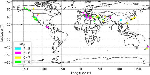
After implementing the previously mentioned data processing steps, the resulting data set contains 23,929 ground-motion records from 325 distinct earthquake events. This refined data set is then employed for the development and execution of the CVAE model. The geographical distribution of these 325 seismic events across the tectonic map is illustrated in Figure 1. Additionally, the focal mechanisms of these earthquakes, categorized based on the rake angle as documented in [25], are summarized in Table 1. The focal mechanism data include 14164 strike-slip events, 484 normal faulting events, 6479 reverse faulting events, 1722 reverse oblique faulting events, and 1080 normal oblique faulting events, all classified according to their respective rake angles.
| Fault mechanism | F | Rake angle range (°) |
|---|---|---|
| Strike slip | 0 | −180 < Rake < −150 to –30 < Rake < 30 |
| Normal | 1 | 150 < Rake < 180 to –120 < Rake < −60 |
| Reverse | 2 | 60 < Rake < 120 |
| Reverse oblique | 3 | 30 < Rake < 60 to 120 < Rake < 150 |
| Normal oblique | 4 | −150 < Rake < −120 to 60 < Rake < −30 |
The CVAE model in this study employs an encoder to synthesize the latent space of the response spectra, including PGA. This encoder network creates the latent space by considering the conditional inputs and their corresponding spectral accelerations as the initial input. However, the transformation from latent space to response spectra relies on a set of conditional inputs, which play a pivotal role in the entire CVAE architecture. These conditional inputs consist of key attributes, such as , , and . These features are crucial for accurately encoding the response spectra and accessing the latent space.
The focal mechanism, also referred to as the mechanism based on the rake angle, is a seismic parameter that describes the orientation of fault slip during an earthquake. This parameter provides essential insights into the tectonic setting and the dynamics of the seismic source, as detailed in Table 1. These classifications are used to quantitatively characterize the focal mechanism of an earthquake, which in turn informs our understanding of the tectonic environment. Figure 2 illustrates the variation of with respect to , elucidating that ground-motion variations become less sensitive to near-field complexities and are affected by regional geological conditions.
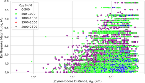
Table 2 presents the statistical measures of the data set, which includes conditional inputs and 24 output variables for spectral acceleration with 5% damping across a range of spectral periods from 0.01 to 4.0 s. Further, the statistical analysis indicates that demonstrates positive skewness, suggesting a significant asymmetry in the data distribution. Additionally, the observed kurtosis value for points to a heavy-tailed distribution, which deviates from a Gaussian distribution.
| Variable | Mean | Standard deviation | Minimum | Maximum | Kurtosis | Skewness | |
|---|---|---|---|---|---|---|---|
| 5.154 | 1.029 | 4.000 | 7.900 | 1.838 | 0.706 | ||
| Hd | 9.946 | 3.706 | 1.800 | 24.000 | 7.197 | 1.450 | |
| (km) | 137.277 | 92.646 | 0.370 | 498.580 | 5.486 | 1.894 | |
| ( | 6.071 | 0.388 | 4.492 | 7.650 | 1.240 | 6.485 | |
| PGA ( | 0.036 | 0.094 | 5.43e-07 | 1.762 | 55.109 | 6.151 | |
| at T = | 0.01 s ( | 0.035 | 0.095 | 5.43e-07 | 1.793 | 55.135 | 6.155 |
| 0.02 s ( | 0.035 | 0.096 | 5.43e-07 | 1.830 | 55.166 | 6.164 | |
| 0.03 s ( | 0.042 | 0.105 | 5.43e-07 | 2.161 | 56.755 | 6.376 | |
| 0.04 s ( | 0.043 | 0.114 | 5.43e-07 | 2.349 | 68.202 | 6.581 | |
| 0.05 s ( | 0.046 | 0.121 | 5.43e-07 | 2.442 | 58.601 | 6.676 | |
| 0.06 s ( | 0.051 | 0.139 | 5.43e-07 | 2.699 | 58.473 | 6.683 | |
| 0.07 s ( | 0.057 | 0.155 | 5.44e-07 | 2.910 | 58.127 | 6.639 | |
| 0.08 s ( | 0.061 | 0.151 | 5.44e-07 | 3.019 | 57.736 | 6.594 | |
| 0.09 s ( | 0.065 | 0.171 | 5.45e-07 | 3.298 | 58.018 | 6.626 | |
| 0.15 s ( | 0.082 | 0.205 | 6.34e-07 | 3.707 | 58.255 | 6.632 | |
| 0.2 s ( | 0.084 | 0.211 | 7.48e-07 | 4.299 | 68.097 | 6.604 | |
| 0.3 s ( | 0.078 | 0.165 | 9.15e-07 | 4.702 | 58.030 | 6.595 | |
| 0.5 s ( | 0.062 | 0.155 | 8.82e-07 | 3.206 | 58.438 | 7.667 | |
| 0.6 s ( | 0.052 | 0.141 | 5.32e-07 | 3.405 | 68.327 | 7.659 | |
| 0.7 s ( | 0.047 | 0.130 | 5.32e-07 | 4.358 | 57.715 | 7.597 | |
| 0.8 s ( | 0.042 | 0.123 | 4.07e-07 | 2.458 | 67.364 | 7.558 | |
| 0.9 s ( | 0.038 | 0.111 | 3.21e-07 | 2.512 | 67.716 | 7.607 | |
| 1.0 s ( | 0.032 | 0.101 | 2.59e-07 | 2.057 | 67.486 | 7.584 | |
| 1.2 s ( | 0.028 | 0.063 | 1.80e-07 | 2.036 | 67.464 | 7.601 | |
| 1.5 s ( | 0.021 | 0.045 | 1.15e-07 | 1.157 | 67.274 | 7.579 | |
| 2.0 s ( | 0.017 | 0.037 | 6.47e-08 | 1.157 | 67.492 | 7.632 | |
| 3.0 s ( | 0.011 | 0.031 | 2.87e-08 | 1.054 | 67.709 | 7.673 | |
| 4.0 s ( | 0.005 | 0.022 | 1.61e-08 | 0.354 | 68.590 | 7.825 | |
- Abbreviation: PGA, Peak Ground Acceleration.
Dhanya and Raghukanth [34] examined the same database and utilized the Shapiro–Wilk method as an initial step to assess the normality of the data. In their methodology, the data points (N) were first arranged in ascending order, and the W statistics were computed following [35]. Using the computed W statistics and the number of data points (N), the mean and standard deviation of the distribution were derived based on the approach outlined by Royston. Their analysis confirmed, with a confidence level of 99%, that the data distribution does not follow a Gaussian distribution. Additionally, the study highlighted the heavy-tailed and skewed nature of the spectral acceleration () distribution, reinforcing the importance of recognizing its deviation from a typical Gaussian model. The positive skewness in the values indicates that there are more instances of lower spectral acceleration values, with fewer occurrences of extremely high values. This skewness reveals an imbalance, where most of the data clusters toward the lower end of the scale, creating a long tail on the higher end. Similarly, the high kurtosis value signifies that the distribution has a propensity for outliers, indicating that extreme values are more frequent than what would be expected in a normal distribution.
CVAEs consist of two main components: the encoder and the decoder. The encoder's role is to create the latent space representation, while the decoder's function is to derive the response spectra back from the derived latent space. These two components undergo simultaneous training, with the encoder striving to encode samples that the decoder tries to back-track, and the decoder aiming to accurately decode the corresponding with good accuracy. This continuous training process drives the encoder to create an increasingly compressed representation of , thereby enhancing the model's ability to capture the complex, multimodal nature of ground-motion recordings.
An additional advantage of CVAEs is their capability to model the entire data distribution, rather than focusing solely on the mean or median, as is often the case with ANNs. By modeling the full data distribution, CVAEs provide a more comprehensive understanding of ground-motion recordings, which can lead to more accurate and reliable representations. This holistic approach to data modeling ensures that the nuances and variations in the data are better captured, ultimately improving the robustness and applicability of the model in real-world scenarios.
Therefore, the use of CVAEs represents a significant advancement over traditional modeling techniques, offering improved performance in scenarios involving complex and multimodal data distributions. Furthermore, CVAEs have the ability to incorporate prior knowledge or constraints into the model, such as physical laws or domain-specific rules. This feature can significantly aid the learning process and enhance the model's performance, especially when working with limited or noisy data. By integrating these constraints, the model can be better guided during training, leading to more accurate and reliable data compression.
However, training CVAEs presents its own set of challenges. It requires meticulous tuning of the model architecture and hyperparameters to achieve optimal performance. This careful calibration is essential to ensure that the model can effectively learn from the data and effectively reproduce the data. Despite these challenges, the potential advantages of using CVAE for capturing complex, multimodal data, such as ground-motion recordings, make it a promising area for future research and application in ground-motion analysis. This is one of the primary objectives of this paper.
The subsequent section of the paper delves into the technical details of the CVAE model. It elaborates on the architecture, the nuances of the training process, and how input parameters are incorporated to accurately represent and encode ground motion. This detailed examination aims to provide a comprehensive understanding of how CVAEs can be effectively employed in the context of ground-motion analysis.
3 Model Construction and Training Strategy
The development of CVAE has been done based on VAE, which represents a powerful class of generative models that learn to approximate complex probability distributions. VAEs are proven to address the fundamental challenges in unsupervised learning, thus helping in capturing high-dimensional data distributions and enabling efficient sampling. To understand the necessity and the foundations of CVAE implementation, it is indeed important to comprehend the functioning of VAE and its technicalities concerning probabilistic modeling. This offers a principled approach to learning the latent variable models and generating new samples. An overview of the network architecture is provided in Figure 3. The corresponding mathematical formulations in the current section are in tune with the preliminary research work [36-38].
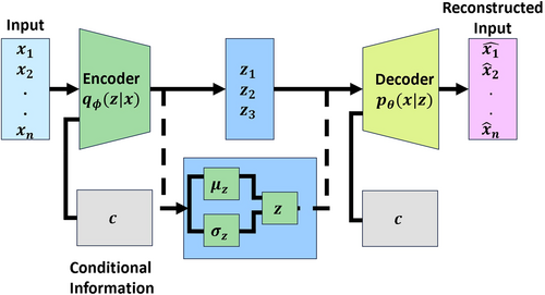
During the training phase, the encoder and decoder networks are jointly optimized to maximize the ELBO. The encoder parameterized by approximates the posterior distribution , while the decoder parameterized by reconstructs the input from samples of .
| ALGORITHM 1Training Conditional Variational Autoencoder (CVAE). | |
|---|---|
| Require: | |
| 1: | Input: Training data set , number of epochs , learning rate , batch size |
| 2: | Initialize parameters (encoder), (decoder) |
| 3: | Initialize the optimizer (Adam) with learning rate |
| 4: | for to do |
| 5: | Randomly shuffle and partition the data set into mini-batches |
| 6: | for each mini-batch do |
| 7: | //Encoder Forward Pass |
| 8: | Compute encoder outputs: |
| 9: | , = encoder() |
| 10: | Sample |
| 11: | Compute latent components: |
| 12: | |
| 13: | //Decoder Forward Pass |
| 14: | Compute decoder outputs: |
| 15: | = decoder() |
| 16: | //Loss Computation |
| 17: | Compute reconstruction loss: |
| 18: | |
| 19: | Compute KL divergence: |
| 20: | |
| 21: | //Total Loss |
| 22: | |
| 23: | //Backward Pass |
| 24: | Compute Gradients: |
| 25: | |
| 26: | Update encoder and decoder parameters using optimizer: |
| 27: | |
| 28: | |
| 29: | end for |
| 30: | end for |
Particularly, VAEs focus on maximizing the ELBO to learn the latent representations. The latent variables are typically Gaussian distributed, which simplifies the computation limits but limits the model's ability to capture complex latent representations. This premise can lead to suboptimal representations, particularly in situations, where the true latent space is non-Gaussian or highly structured. Along with the same, the aforementioned phenomenon of mode collapse occurs when the decoder fails to utilize the entire latent space efficiently, resulting in the generation of limited and repetitive samples. This issue arises because VAEs prioritize reconstruction over latent space exploration, leading to poor diversity in generated outputs. While the VAEs aim to learn the disentangled representations, ensuring that each latent variable corresponds to a meaningful and independent feature of the data remains challenging. In practice, it is often observed that latent variables often capture mixed or irrelevant factors, hindering the interpretability and generative performance of the developed model.
To address the following challenge, CVAE is used to extend the aforementioned VAE framework detailed above by incorporating conditional information in both the encoder and decoder. This extension allows for more flexible and precise modeling of data distributions, particularly in tasks requiring structured outputs or fine-grained control over generated samples. This is more vital in the accurate representation of the data.
Therefore, CVAEs exhibit greater flexibility in modeling diverse data distributions compared with standard VAEs. The conditional framework allows for the incorporation of structured information and temporal dependencies, resulting in more accurate and context-aware generation of .
Along with the same, the incorporation of also resolves the problem of mode collapse by encouraging the exploration of diverse regions in the latent space corresponding to different conditions. This leads to more varied and realistic samples compared with traditional VAEs.
On the other hand, the decoder network reconstructs the input data from sampled latent variables conditioned on . The likelihood function models the conditional distribution of given and . It is typically parameterized by and outputs the parameters of the data distribution, like, mean and variance.
This transformation ensures that the predicted values remain nonnegative and better align with the true distribution of ground-motion data. The final spectral acceleration values are obtained by exponentiating the decoder's outputs. This log-normal assumption improves numerical stability, reduces bias in reconstruction, and enhances the model's ability to learn skewed distributions, making it a better fit for ground motion modeling.
-
Encoder and decoder initialization: The algorithm starts by initializing the parameters for the encoder and for the decoder. These parameters will be updated iteratively during training.
-
Mini-batch training: The data set is partitioned into mini-batches of size 32 (number of samples). For each mini-batch, the encoder computes the parameters and of the conditional posterior .
-
Reparameterization and latent variable sampling: Using the reparameterization trick, latent variables are sampled from the Gaussian distribution with mean and standard deviation .
-
Decoder output: Given and , the decoder computes the parameters and of the conditional likelihood .
-
Loss computation: The algorithm calculates two components of the loss function. The first component is the that penalizes the deviation of from . The second component is the reconstruction loss (), which measures how well the decoder reconstructs from and .
-
Gradient calculation and update: The gradients ( and ) of the total loss () with respect to and are computed and used to update the encoder and decoder parameters using an optimizer with a learning rate , obtained through iterative implementation.
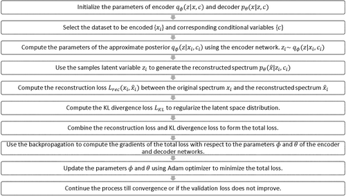
The complete methodology has been summarized in Figure 4, elucidating the steps from ground motion recording to representation of . The optimal parameters of the CVAE model were determined through a systematic process involving hyperparameter tuning, which is a widely accepted practice in ML model optimization. Initially, a broad range of values for key hyperparameters, such as learning rate, latent space dimensions, and the number of neurons in each layer, were explored using grid search and random search strategies. Figure 5 depicts a scatterplot illustrating Recorded vs. Predicted Sa values for both training and validation sets of the data.
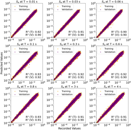
To refine the architecture of the CVAE with seven conditional inputs and 24 outputs, we conducted an extensive grid search to optimize key hyperparameters. The input and output layers were fixed at 24 neurons, corresponding to the input and output dimensionality. The grid search focused on the number of neurons in the hidden layers of both the encoder and decoder, progressively reducing the layer sizes after the initial 24-neuron input and output layers. In the encoder, the input layer was set to 24 neurons, and Hidden Layer 1 was explored with a range of 16–8 neurons, with a step size of 4. Hidden Layer 2 varied between 12 and 6 neurons, with a step size of 3. The latent variable layer was fixed at three neurons, corresponding to the three latent variables.
For the decoder, the output layer remained at 24 neurons, and Hidden Layer 1 ranged from 16 to 8 neurons, while Hidden Layer 2 was adjusted between 12 and 6 neurons. This process is an exact replica of the above information with respect to the encoder.
We also tested learning rates of 0.0001 and 0.0002, as well as dropout rates of 0.2 and 0.3, to analyze their impact on model accuracy and stability. After evaluating all configurations, the optimal settings were found to be: for the encoder, an input layer size of 24 neurons, Hidden Layer 1 with 12 neurons, Hidden Layer 2 with six neurons, and a latent variable layer of three neurons. The decoder architecture was arranged symmetrical to the encoder architecture. The optimal learning rate was 0.0001, and the ideal dropout rate was 0.2.
A fivefold cross-validation was employed to ensure that the model's performance generalizes well across unseen data, minimizing overfitting risks. Furthermore, early stopping was utilized during training to prevent the model from overfitting by monitoring validation loss and halting the process once the performance plateaued. This approach, grounded in empirical experimentation and rigorous evaluation, ensures the selection of parameters that strike a balance between bias and variance, enhancing the model's predictive accuracy and robustness.
4 Evaluation of Model Performance
Frank and Todeschini [39] argue that a crucial criterion for robust model training is maintaining a ratio, where the number of input parameters surpasses the number of data samples. In their study, they utilize a data set comprising 23,929 data samples and seven input parameters, a configuration that comfortably satisfies this requirement. In the context of ground motion modeling, residual analysis is an essential tool to assess the model's predictive performance. Residuals are calculated as the difference between observed and predicted values, and they provide insights into model bias and variability. Specifically, mixed-effects models are commonly used to account for variability in the data arising from different sources. These models separate the residuals into two components: interevent residuals and intraevent residuals. Interevent residuals capture the variability between different seismic events, influenced by event-specific factors, such as magnitude and fault mechanism. Intraevent residuals, on the other hand, reflect variability within a single event and are driven by site-specific factors, such as local soil conditions and path effects. By employing a mixed-effects approach, the model can isolate these two sources of variability, enhancing its accuracy and reliability.
For this study, residuals were computed following the mixed-effects methodology described in [25]. This approach facilitates an in-depth evaluation of prediction errors by distinguishing between event-driven and location-driven uncertainties, which is critical for improving seismic hazard assessments. Figure 6 illustrates the distribution of interevent residuals for PGA and across various time intervals of interest. These boxplots, depicting both the mean and standard deviation, provide a concise visual overview of the data's statistical spread and central tendency. An important observation is the absence of discernible patterns in the mean values across different spectral periods, indicating that the model's predictions are unbiased with respect to . This consistency ensures the reliability and validity of the model in ground-motion prediction.
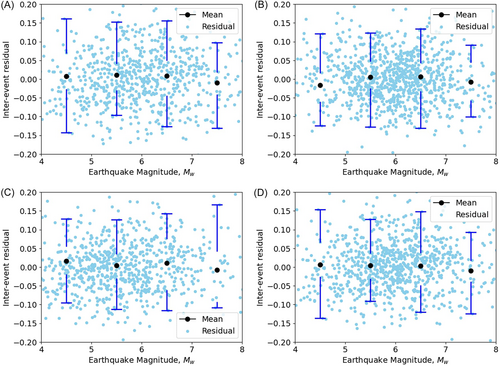
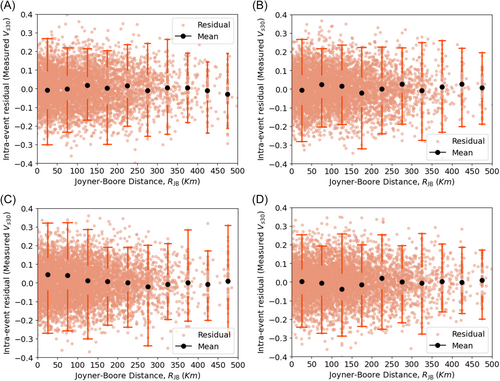
Similarly, residuals were analyzed concerning the Joyner–Boore distance () and the time-averaged shear-wave velocity (), with bin widths selected to capture significant variability. Figures 7-10 illustrate the relationship between these ground-motion parameters and the residuals. The uniform distribution of mean intraevent residuals with respect to and , similar to the interevent residuals with respect to moment magnitude (), suggests that the model does not introduce systematic bias. Moreover, the analysis indicates lower variability among interevent residuals compared with intraevent residuals, further supporting the model's robustness. These findings reinforce the model's reliability for practical applications in seismic hazard assessments.
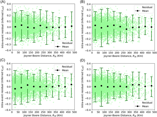
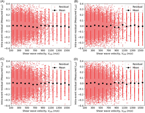
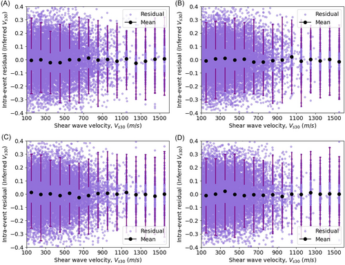
is the total standard deviation for measured ,
is the total standard deviation for inferred ,
τ is the interevent residual,
is the intraevent standard deviation for measured , and
is the intraevent standard deviation for inferred .
The examination of standard deviations is provided in Table 3, which offers valuable insights into the diversity of ground-motion parameters. The smaller interevent standard deviation in comparison to the intraevent standard deviation suggests that variations between different seismic events are less pronounced than those within a single event. This pattern may indicate a more consistent seismic source or path effects across different events. Furthermore, the finding that the standard deviation for directly measured values is narrower than that for inferred values implies that direct measurements offer a more dependable assessment of site conditions.
| Parameter | τ | |||||
|---|---|---|---|---|---|---|
| PGA | 0.147 | 0.287 | 0.322 | 0.306 | 0.339 | |
| at T = | 0.01 s | 0.161 | 0.274 | 0.318 | 0.320 | 0.358 |
| 0.02 s | 0.123 | 0.245 | 0.274 | 0.279 | 0.305 | |
| 0.03 s | 0.136 | 0.272 | 0.304 | 0.280 | 0.311 | |
| 0.04 s | 0.106 | 0.265 | 0.285 | 0.280 | 0.299 | |
| 0.05 s | 0.131 | 0.243 | 0.276 | 0.287 | 0.315 | |
| 0.06 s | 0.117 | 0.258 | 0.283 | 0.329 | 0.349 | |
| 0.07 s | 0.109 | 0.279 | 0.300 | 0.301 | 0.320 | |
| 0.08 s | 0.144 | 0.286 | 0.320 | 0.302 | 0.335 | |
| 0.09 s | 0.134 | 0.260 | 0.292 | 0.281 | 0.311 | |
| 0.15 s | 0.136 | 0.263 | 0.296 | 0.273 | 0.305 | |
| 0.20 s | 0.159 | 0.252 | 0.298 | 0.291 | 0.332 | |
| 0.30 s | 0.101 | 0.255 | 0.274 | 0.303 | 0.319 | |
| 0.50 s | 0.115 | 0.260 | 0.284 | 0.308 | 0.329 | |
| 0.60 s | 0.130 | 0.240 | 0.273 | 0.277 | 0.306 | |
| 0.70 s | 0.116 | 0.246 | 0.272 | 0.286 | 0.309 | |
| 0.80 s | 0.139 | 0.266 | 0.300 | 0.303 | 0.333 | |
| 0.90 s | 0.100 | 0.268 | 0.286 | 0.316 | 0.331 | |
| 1.00 s | 0.140 | 0.290 | 0.322 | 0.317 | 0.347 | |
| 1.20 s | 0.135 | 0.254 | 0.288 | 0.324 | 0.351 | |
| 1.50 s | 0.117 | 0.255 | 0.281 | 0.314 | 0.335 | |
| 2.00 s | 0.137 | 0.279 | 0.311 | 0.303 | 0.333 | |
| 3.00 s | 0.149 | 0.253 | 0.294 | 0.276 | 0.314 | |
| 4.00 s | 0.150 | 0.274 | 0.312 | 0.283 | 0.320 | |
- Abbreviations: PGA, Peak Ground Acceleration; TSI, total standard deviation for inferred; TSM, total standard deviation for measured.
The assumption of a consistent standard deviation, based on an equal distribution of data points across each period, is challenged by observed fluctuations, highlighting the impact of temporal factors on ground-motion characteristics. Variability in site conditions likely contributes to these deviations, underscoring the necessity of accounting for ergodicity in GMMs.
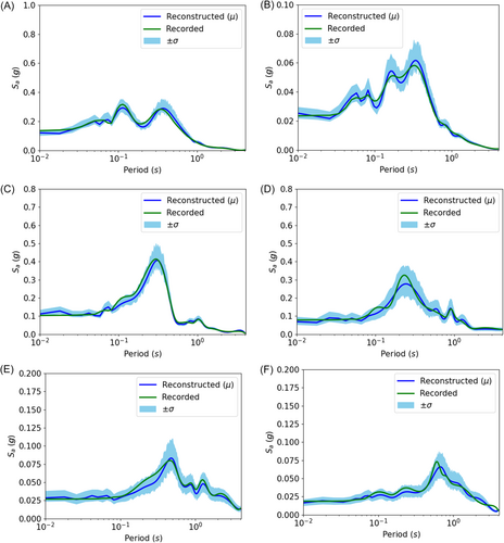
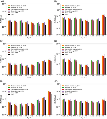
Despite these fluctuations, the model's capacity to predict ground motion impartially across various input variables indicates a robust and dependable framework for seismic hazard evaluation and reconstruction of ground motions. Figure 11 illustrates a few examples comparing the recorded spectral accelerations and their reconstructed counterparts using CVAE. Further, the improved performance of CVAE in comparison with well-known GMMs [40-44] has been established in Figure 12 with the help of seismological misfits as derived by Karimzadeh et al. [45]. Also, Table 4 provides a quantitative comparison of CVAE with various ML–based GMMs, such as ANN, Kernel–Ridge Regressor, Random Forest Regressor, Support Vector Regressor, and an ensemble model [46]. We utilized Mean Square Error (MSE) and Mean Absolute Error to quantitatively test the predictive capabilities of CVAE. Further, the CVAE model was validated against a collected database of Turkey and Ridgecrest [47, 48] earthquakes. The resultant MSE values for various GMMs on a collected database of Turkey and Ridgecrest are provided in Table 5.
| Model | Mean square error | Mean absolute error | score |
|---|---|---|---|
| ANN | 0.6350 | 0.6297 | 0.8799 |
| KRR | 0.6439 | 0.6328 | 0.8768 |
| RFR | 0.5247 | 0.5599 | 0.9026 |
| SVR | 0.6472 | 0.5351 | 0.8759 |
| Ensemble | 0.5818 | 0.5994 | 0.8897 |
| CVAE | 0.5068 | 0.5204 | 0.9153 |
- Abbreviations: ANN, Artificial Neural Network; CVAE, Conditional Variational Autoencoder; KRR, Kernel–Ridge Regressor; RFR, Random Forest Regressor; SVR, Support Vector Regressor.
| Model | Earthquake | Metric | PGA | at | at | at |
|---|---|---|---|---|---|---|
| I14 [44] | Turkey | MSE | 0.568 | 0.634 | 0.685 | 0.671 |
| MAE | 0.611 | 0.628 | 0.655 | 0.662 | ||
| Ridgecrest | MSE | 0.244 | 0.374 | 0.568 | 0.609 | |
| MAE | 0.393 | 0.486 | 0.631 | 0.654 | ||
| CB14 [42] | Turkey | MSE | 0.411 | 0.580 | 0.517 | 0.404 |
| MAE | 0.528 | 0.604 | 0.572 | 0.496 | ||
| Ridgecrest | MSE | 0.261 | 0.343 | 0.379 | 0.331 | |
| MAE | 0.407 | 0.463 | 0.467 | 0.467 | ||
| BSSA14 [41] | Turkey | MSE | 0.399 | 0.630 | 0.495 | 0.422 |
| MAE | 0.505 | 0.627 | 0.562 | 0.509 | ||
| Ridgecrest | MSE | 0.229 | 0.362 | 0.364 | 0.355 | |
| MAE | 0.383 | 0.470 | 0.471 | 0.490 | ||
| ASK14 [40] | Turkey | MSE | 0.429 | 0.893 | 0.767 | 0.468 |
| MAE | 0.541 | 0.766 | 0.712 | 0.546 | ||
| Ridgecrest | MSE | 0.246 | 0.348 | 0.401 | 0.321 | |
| MAE | 0.401 | 0.461 | 0.479 | 0.450 | ||
| CY14 [46] | Turkey | MSE | 0.529 | 0.656 | 0.499 | 0.424 |
| MAE | 0.600 | 0.647 | 0.562 | 0.501 | ||
| Ridgecrest | MSE | 0.259 | 0.333 | 0.354 | 0.316 | |
| MAE | 0.394 | 0.456 | 0.463 | 0.447 | ||
| SP23 [46] | Turkey | MSE | 0.434 | 0.557 | 0.462 | 0.396 |
| MAE | 0.504 | 0.585 | 0.549 | 0.494 | ||
| Ridgecrest | MSE | 0.232 | 0.350 | 0.363 | 0.324 | |
| MAE | 0.377 | 0.462 | 0.462 | 0.450 | ||
| ANN [46] | Turkey | MSE | 0.421 | 0.599 | 0.537 | 0.411 |
| MAE | 0.497 | 0.605 | 0.591 | 0.517 | ||
| Ridgecrest | MSE | 0.238 | 0.414 | 0.403 | 0.330 | |
| MAE | 0.389 | 0.512 | 0.511 | 0.466 | ||
| KRR [46] | Turkey | MSE | 0.454 | 0.608 | 0.471 | 0.420 |
| MAE | 0.529 | 0.619 | 0.553 | 0.509 | ||
| Ridgecrest | MSE | 0.246 | 0.364 | 0.369 | 0.320 | |
| MAE | 0.389 | 0.476 | 0.478 | 0.450 | ||
| RFR [46] | Turkey | MSE | 0.536 | 0.567 | 0.519 | 0.433 |
| MAE | 0.558 | 0.585 | 0.577 | 0.525 | ||
| Ridgecrest | MSE | 0.317 | 0.391 | 0.782 | 0.539 | |
| MAE | 0.447 | 0.491 | 0.687 | 0.575 | ||
| SVR [46] | Turkey | MSE | 0.459 | 0.584 | 0.507 | 0.446 |
| MAE | 0.527 | 0.608 | 0.568 | 0.518 | ||
| Ridgecrest | MSE | 0.238 | 0.367 | 0.379 | 0.328 | |
| MAE | 0.380 | 0.475 | 0.487 | 0.461 | ||
| CVAE | Turkey | MSE | 0.406 | 0.561 | 0.475 | 0.403 |
| MAE | 0.512 | 0.604 | 0.585 | 0.504 | ||
| Ridgecrest | MSE | 0.212 | 0.345 | 0.352 | 0.312 | |
| MAE | 0.379 | 0.472 | 0.482 | 0.461 |
- Abbreviations: ANN, Artificial Neural Network; CVAE, Conditional Variational Autoencoder; GMM, Ground Motion Model; KRR, Kernel–Ridge Regressor; MAE, Mean Absolute Error; MSE, Mean Square Error; PGA, Peak Ground Acceleration; RFR, Random Forest Regressor; SVR, Support Vector Regressor.
5 Latent Space Analysis
Assessing the CVAE model's effectiveness in reconstructing ground motion requires a thorough examination of the various factors that influence seismic responses. These factors, which include , condition the latent space representation of the model. By using these inputs, the model reconstructs ground-motion values that are critical for seismic hazard evaluation and engineering applications. The CVAE's ability to encapsulate the interdependencies between these parameters and the ground-motion values is pivotal for enhancing the precision of seismic risk assessments and understanding the underlying physical mechanisms that drive seismic activity.
The current CVAE model contains three latent variables (, and ). Figure 13 illustrates the variation of latent space variables and with respect to the six variables discussed above. The latent space analysis provides a detailed exploration of how the latent variables respond to different conditional inputs, revealing trends and relationships that are essential for evaluating seismic hazards under varying conditions. As increases, indicating larger seismic events, the distribution of latent variables shifts to reflect the heightened ground-motion intensity. Deeper seismic events cause different patterns in the latent space, reflecting how depth influences energy dissipation and ground-motion characteristics. Greater distances from the fault result in a reduction in ground-motion intensity, a trend that is captured by the latent space representation as it reflects attenuation effects. The inclusion of is crucial for understanding ergodic effects, as lower velocities correspond to softer soils and amplified ground motions, a relationship that is clearly depicted in the latent space variables. The direction of ground-motion records (horizontal or vertical) affects the latent space distribution, reflecting the inherent differences in ground-motion characteristics between these two directions. The type of faulting mechanism also significantly influences the latent space, showing how different tectonic settings impact ground motion.
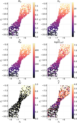
The analysis of trends in the latent space offers a nuanced understanding of seismic responses across diverse conditions. By examining the relationships between the latent variables and the conditional inputs, we gain insight into how the model captures key seismic phenomena, such as magnitude scaling, distance attenuation, soil amplification, and fault mechanisms. Notably, categorical input variables like and show a significant influence on the latent variables. However, compared with continuous variables, such as , categorical inputs impact the latent representation in a more discrete manner. Continuous variables, on the other hand, exhibit smoother gradients in the latent space plots, reflecting their continuous nature and gradual impact on the model's representations.
The latent space framework of the CVAE provides valuable insights into how ground-motion data can be compressed and reconstructed, accurately capturing the complex interdependencies of seismic parameters. The detailed latent space visualization also underscores the model's ability to capture underlying physical processes for exploring how seismic parameters influence ground-motion behavior.
In addition to its reconstruction capabilities, Section 6 of this study presents a parametric analysis of the CVAE model, which will detail the impact of various input parameters. This analysis will provide further insights into the model's performance under different seismic scenarios.
6 Parametric Analyses
In designing a CVAE for predicting , a novel adaptation has been introduced to modify the conventional CVAE framework for this specific task. Traditionally, CVAEs are designed for data compression and reconstruction rather than direct regression or prediction tasks [37, 38]. Their latent space representation is primarily optimized for generating variations of input data rather than mapping input variables to precise target values.
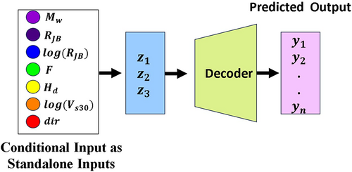
To bridge this gap, we propose an innovative Mapping Network, which enables the CVAE to perform prediction tasks while still leveraging its generative properties. This mapping network integrates conditional inputs directly into the latent space, ensuring that the decoder can generate spectral acceleration predictions informed by seismic parameters. Specifically, the seven input variables are first processed through an intermediate transformation layer with four neurons before being mapped into a three-neuron latent space. This structured transformation allows the CVAE to retain the ability to model complex relationships between variables while ensuring that the latent space remains meaningful for prediction.
By freezing the decoder weights, the model effectively learns a structured latent representation, which enables accurate spectral acceleration predictions from conditional inputs. This modification extends the applicability of CVAEs beyond their traditional role as generative models, making them suitable for predictive modeling in seismic analysis. Previous studies [49, 50] have demonstrated that CVAEs, in their standard form, are not inherently suited for regression tasks. However, our approach overcomes this limitation, demonstrating how a modified CVAE architecture can be successfully adapted for direct predictive modeling in earthquake engineering applications.
By freezing the weights on the decoder side of the CVAE, the model retains its ability to generate accurate spectral acceleration predictions. This approach effectively combines the strengths of the CVAE's data compression with a tailored prediction mechanism, thus enhancing the model's applicability for earthquake spectral analysis. This novel methodology demonstrates a practical adaptation of generative models for predictive tasks. The same procedure has been illustrated in Figure 14.
The assessment of the proposed model for ground-motion prediction involves an in-depth examination of various input parameters that impact seismic responses. These parameters include , , average shear-wave velocity up to 30 m , and . By testing different combinations of these parameters, the model can forecast ground-motion values essential for seismic hazard evaluation and engineering design. The model's ability to capture the intricate relationships between these parameters and ground motion is crucial for understanding the underlying physical phenomena and enhancing the precision of seismic risk predictions. Figures 15-18 illustrate the model's performance across different scenarios.
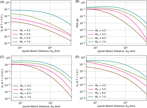
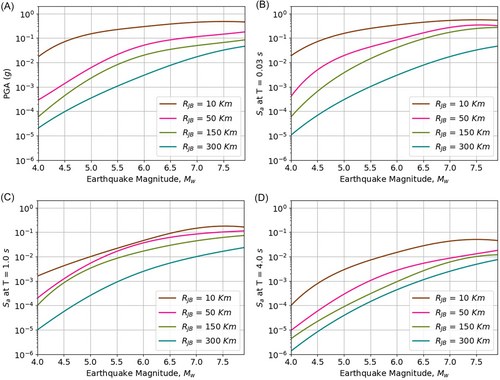
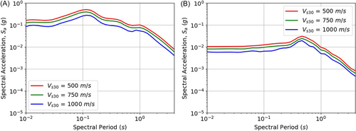
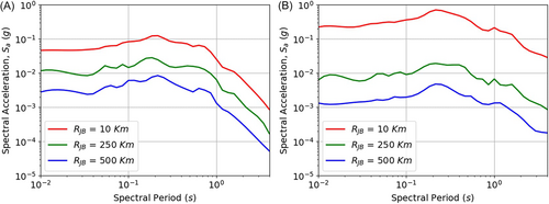
Figure 15 presents a detailed analysis of ground-motion parameters, focusing on PGA and at various spectral periods, which are vital for seismic hazard assessment. The parameters are assessed with respect to and different values of , offering insights into the seismic response under various conditions.
Evaluating , which represents the average shear-wave velocity in the top 30 m of the soil, along with , is crucial for understanding seismic responses. The study's emphasis on strike-slip faults, characterized by horizontal movement, and the analysis of relative to across various combinations in Figure 16, provides additional depth to the seismic risk evaluation. The observed variations for of 550 and of 5.5 km refine the understanding of ground-motion characteristics. The analysis shows that the model effectively captures variations in ground-motion values in relation to and . As increases, indicating stronger ground movement, the model predicts a rise in ground-motion values. Conversely, with an increase in , representing a greater distance from the seismic source, the model forecasts a decrease in ground-motion levels. To investigate the impact of site conditions on ground motion, Figure 17 analyses variations across different soil classes. Figure 17 illustrates how spectral acceleration () varies across different soil classes, characterized by values of 500, 750, and 1000 . This analysis is essential in understanding how site conditions influence ground motion. The figure presents separate plots for strike-slip and reverse fault mechanisms, allowing for a comparative evaluation of the influence of fault type on seismic response. It is observed that softer soils (lower ) tend to amplify ground motion, leading to higher values, whereas stiffer soils (higher ) exhibit lower amplification effects. This result aligns with established site response theories and reinforces the model's ability to capture soil-dependent seismic variations. Finally, Figure 18 explores the variation in with different distances for both strike-slip and normal faulting mechanisms. The figure illustrates how spectral acceleration () systematically decreases as increases, highlighting the expected attenuation of ground motion with increasing distance from the seismic source. Additionally, the trends for strike-slip and normal faulting mechanisms are compared, revealing any potential differences in ground-motion characteristics between these fault types. These observations provide further insights into how faulting style influences ground-motion attenuation, complementing the earlier discussions on and fault mechanisms in Figures 16 and 17.
7 Conclusions
In this study, a CVAE-based approach is employed to reconstruct a 5% damped spectral acceleration from ground-motion records sourced from the NGA-West2 database. The evaluation of the CVAE model focuses on its ability to faithfully reconstruct the observed response spectra, assessed through residual analysis to ensure unbiased performance relative to the input variables. The generative capabilities of the CVAE-based model offer significant advantages over deterministic and rule-based reconstruction methods. Notably, the model demonstrates a reduction in misfits compared with conventional techniques, highlighting its enhanced fidelity in capturing complex spectral patterns. Furthermore, benchmarking against established GMMs in similar seismotectonic settings validates the efficacy and robustness of the CVAE approach.
However, a key observation in this study is the smoothing effect introduced by the CVAE when generating response spectra across different spectral periods. This behavior, as seen in Figures 15 and 16, can be attributed to the probabilistic nature of the CVAE, where the learned latent space encodes global spectral trends but may suppress fine-grained variations, particularly for long-period motions. Additionally, the observed plateau in for large magnitudes arises due to the model's dependence on data-driven learning, which differs from traditional GMMs that explicitly parameterize magnitude scaling. These effects underscore a fundamental difference between empirical models and deep generative approaches—while the CVAE offers flexibility and improved spectral representation, it also introduces unique challenges in capturing extreme variations.
While the CVAE model has demonstrated its effectiveness in reconstructing ground motion, several aspects need to be addressed in future research. One critical consideration is the inherent challenge of deep learning models, such as the CVAE, in handling extrapolation regions. Predictions for scenarios with sparse or unobserved data, such as large magnitudes and short distances, may exhibit reduced accuracy, as the model relies heavily on patterns learned from the training data set. This limitation highlights the need for caution when interpreting results in such regions, particularly in engineering applications. Future research could explore ways to mitigate this issue by integrating physics-based constraints or augmenting the training data to better capture extreme cases.
Additionally, the model's reliance on the NGA-West2 data set, which is region-specific, restricts its generalizability. Expanding the model's training to include global data sets could improve its applicability across different seismic regions, enhancing its utility for broader seismic hazard assessments. Another area for improvement is the model's handling of nonlinear soil effects, which significantly influence spectral acceleration, particularly in soft soil conditions. The current approach does not explicitly account for these nonlinear effects. Incorporating nonlinear site response models in future research could enhance prediction accuracy for diverse soil profiles.
Furthermore, while the CVAE model effectively captures complex dependencies in ground-motion data, its impact on uncertainty reduction remains an area for further investigation. Our analysis indicates that while the model structures the latent space efficiently, the changes in interevent and intraevent residuals remain relatively small. This suggests that the model does not significantly reduce overall uncertainty compared with the existing literature [34] but rather provides a more flexible and data-driven representation of spectral variations. A more detailed exploration of uncertainty decomposition, including comparisons with existing methodologies, could provide further insights into how deep generative models contribute to ground motion modeling.
Addressing these challenges in future research will not only improve the robustness of the model but also expand its potential applications in seismic hazard assessments globally.
Author Contributions
Pavan Mohan Neelamraju: formal analysis, investigation, writing – original draft preparation. Akshay Pratap Singh: formal analysis, investigation. STG Raghukanth: conceptualization, methodology, review and editing, supervision. All authors read and approved the final manuscript.
Ethics Statement
The authors have nothing to report.
Conflicts of Interest
The authors declare no conflicts of interest.
Open Research
Data Availability Statement
The data sets utilized in this study were gathered and processed by the Pacific Earthquake Engineering Research (PEER) Center and can be accessed online at http://peer.berkeley.edu/ngawest2/databases/. The code is available at https://github.com/thunder-volt/CVAE.


