Physical-Guided Coupling Neural Network Approach for Seismic Wave Propagation
ABSTRACT
Seismic wave propagation is mainly studied by two paradigms: empirical research based on in-situ observation and model test, theoretical research based on mathematical deduction and numerical simulation. However, these paradigms face challenges such as sparse data samples, weak generalization of results, and insufficient understanding of laws. To address these challenges, we propose a coupling neural network that embeds both physical information and constrains physical laws. We use this neural network to learn the law of seismic wave propagation from a combination of theoretical equations and test records. We develop a prediction model of seismic wave propagation that jointly constrains multi-type sparse data, which improves the physical interpretability and extrapolation ability. The results demonstrate that the physical-guided coupling neural network can effectively and flexibly integrate theoretical, simulated, and experimental data, and generate the full waveform data and spatial distribution patterns of various physical quantities, thereby reducing the uncertainty of sparse sensor test data and solving the problem of data interaction of independent research paradigms.
1 Introduction
The simulation of seismic wave propagation is a crucial issue for the field of earthquake engineering. Forward modeling of seismic waves involved solving the wave equation with initial and boundary conditions. Currently, numerical discretization of partial differential equations has made significant progress in simulating physics problems. Numerous researchers have explored various numerical methods for simulating seismic wave propagation, including finite difference methods [1], finite element methods [2], and spectral element methods [3, 4]. These numerical simulation techniques used finite sets of basic functions and corresponding parameters to approximate solutions to partial differential equations, transforming continuous variable analytical problems into numerical problems solved using discrete variables. They excelled in terms of solution accuracy; however, modeling and predicting the evolution of nonlinear multiscale systems using classical analytical or computational tools remain challenging. This included dealing with complex meshing, high-dimensional problems controlled by parameterized partial differential equations, etc. These numerical methods also face challenges in solving inverse problems, which often require repeated forward calculations.
With advancements in computer performance and the development of artificial intelligence and machine learning methods, many scientists are now exploring the potential of using machine learning to address seismic wave propagation problems [5-7]. Scientifically oriented artificial intelligence, as a new interdisciplinary field, combines physical principles with data to construct more general and interpretable machine learning models. To overcome the data dependency issue in traditional machine learning, Raissi et al. [8] developed the universal Physics-Informed Neural Network (PINN) framework. Compared with traditional numerical solutions to partial differential equations, PINNs have the characteristics of not requiring a mesh, which opens up opportunities for applications the traditional numerical methods are challenged with, such as complex domains, solving inverse problems, etc.
In recent years, PINNs have been applied in geophysics [9], solid mechanics [10-12], fluid dynamics [13-15], and heat conduction [16]. Previously, several studies have successfully used PINNs to solve the various forms of the wave equation. Rao et al. [11] used a DNN composite approach to enforce initial and boundary conditions, achieving the propagation of elastic waves in finite domains. Ren et al. [17] employed a PINN model for semi-infinite domain seismic wave simulations without requiring labeled data. Moseley et al. [18] proposed the FBPINN extension, combining domain decomposition and individual subdomain normalization to solve pressure responses in two-dimensional acoustic media. Ding et al. [19] effectively applied the PCNN method to impose free surface stress boundary conditions, enabling the propagation of plane waves and cylindrical waves in elastic half-spaces. Rasht-Behesht et al. [20] achieved full waveform inversion simultaneously during forward modeling by incorporating sensor data into the network. These developments highlight the potential of machine learning approaches in advancing our understanding of seismic wave propagation and enhancing earthquake engineering practices.
PINNs have addressed the limitations of traditional neural network algorithms by embedding physical information, enabling the learning of data scarcity and physical constraints. This approach also alleviates overfitting, reduces the need for large training datasets, and improves the robustness of the training model to achieve reliable predictions. However, due to the addition of partial differential equations and initial boundary value conditions to the loss function, PINNs redefine the solution as the minimum of a loss function to obtain the weights of deep neural networks (DNNs). This may result in inaccurate approximations or incomplete convergence. To address these challenges, many studies have attempted to improve the convergence or solution efficiency of PINNs, such as adaptive sampling approaches [21-23], adaptive activation functions [14, 15, 24], and methods to alleviate the high-frequency hard-to-learn problem [12]. Ding et al. [25] further demonstrated the effectiveness of combining SA-PINNs with spectral element methods (SEMs) to solve one- and two-dimensional wave equations considering complex terrain in a semi-infinite domain. Moreover, Song et al. successfully employed PINNs to model the frequency-domain acoustic VTI wave equation in anisotropic media [26], highlighting the potential of PINNs in handling complex anisotropic wave propagation problems. Building on this foundation, Song et al. extended their research to simulate multicomponent elastic seismic wavefields using deep learning techniques [27], demonstrating the capability of PINNs to accurately model elastic wave propagation in heterogeneous media. These studies, along with others that optimized the network structure for different partial differential equations, show that PINNs can better adapt to various physical problems, including those involving frequency-domain wave equations in anisotropic and elastic media.
Dynamic centrifuge test [28-30] or shaking table test [31, 32] is also an effective means to study the problem of seismic fluctuations, through the deployment of various sensors to obtain the time history data of each point in the soil. By conducting experiments on a centrifuge, we can simulate the propagation of seismic waves in soil and observe the time history data at various points within the soil. However, centrifuge tests come with challenges, such as limited sensor quantities, the presence of complex scattering fields due to sensors and wires, and differences from the original field site. The sensors at each station location can obtain ground motion time history data, so how to study ground motion propagation through time history data is also very important for seismology and earthquake engineering. However, due to the fact that the centrifuge is scaled on the basis of the original site, the presence of sensors and lines makes the process of seismic wave propagation in the soil produce a complex scattering field that is not present in the original site, which makes the obtained test data different from the data of the real earthquake. At the same time, due to the limitation of test conditions, fewer sensors are laid out, and the data obtained is limited. Under the framework of neural network solving, to solve the problem of small datasets, many scientists have made corresponding attempts to solve it.
Cui et al. [33] developed a mechanism and data-driven fusion model to predict charging capacity and energy curves over the full life cycle of batteries in the case of only knowing the planned cycling protocol without any usage history. Xiong et al. [34] augmented the frequency and attenuation information in the kinetic equation by assuming the elasticity coefficient of the constitutive relationship by assuming the wave equation. Jia et al. [35] proposed a physics-guided recurrent neural network model (PGRNN), which adds a density-depth constraint relationship with a small amount of observational data to predict the dynamic relationship of lake temperature. Gou et al. [36] used a Bayesian physics-based neural network based on the program-function equation to infer the velocity field and reconstruct the travel time field.
In this paper, we propose a Physics-Guided Coupled Neural Network (PGCNN) to enhance the simulation of seismic wave propagation. By embedding physical laws directly into the neural network architecture, PGCNN ensures that solutions adhere to fundamental physical principles, reducing unphysical outcomes and improving reliability, especially with sparse data. Notably, this multi-paradigm approach, combining theoretical models and experimental data through hard embedding of physical constraints and soft constraints of physical information, has not been previously applied in the field of seismic wave solving and earthquake engineering. This novel method enables the handling of multi-type coefficient data, facilitating the acquisition of full waveform data and spatial distribution patterns, effectively reducing uncertainties in sparse sensor test data. Additionally, PGCNN incorporates advanced optimization strategies, enhancing convergence rates and computational efficiency. Through both synthetic and real-world experiments, PGCNN demonstrates its effectiveness in reconstructing seismic wave propagation patterns, providing a robust solution for cross-paradigm applications in earthquake engineering.
2 Methodology
2.1 Physical-Guided Coupling Neural Network

When modeling wave propagation in half-space or complex topography using PINNs, the free-surface BC may fail to contribute, leading to the disappearance of reflected waves. With the traditional PINN method, the boundary condition is invalidated if there are only sparse points. So in this paper, we used PCNNs [19] to hard-embed the free surface boundary condition. So that the general boundary condition term does not belong to the loss function. And we use an adaptive training algorithm [27] to determine the coefficients of other loss function terms.
At the bottom of the model, we input a Richer wave with a frequency of 2 Hz, and the time history data of each point in the lower region in the first 3 s can be obtained through the formula, and the time history data of seven sporadic positions are selected as the equivalent applied ricker wave input, as shown in Figure 2. The ordinate of the selected point is [0 m, 5 m, 10 m, 15 m, 20 m, 25 m, 30 m]. The Sobol sequence algorithm [38] was used for the spatio-temporal sampling of the PDE residual loss term, and the uniform sampling method was applied to the data and initial condition terms. The activation functions in the neural network approximating the state variables u are chosen as the Tanh activation functions. With the well-defined loss function as Equation (2), the Adam [39] and LBFGS [40] optimizers are used to find the appropriate parameters for the neural network. It is challenging to train the neural network due to the different scales of the state variables and the corresponding equation residuals. Here, we use the normalization by the maximum value of the state variable u and the wave velocity normalization method to mitigate this problem. All the numerical implementations in this paper are coded in Pytorch [41] and performed on an NVIDIA V100 Tensor core GPU. Appendix A provides a summary of the DNN hyperparameters, case settings, and work-clock time comparisons for all the cases examined in this study.

The total duration of the calculation was 6.0 s. In this case, we first use the neural network to approximate the first 3 s and store the trained network parameters. This can be considered as a “warm start” search for admissible trainable parameters of the network. Then the network is re-trained by inheriting the trained parameters. The first stage of this training strategy is equivalent to training a reusable seismic source, which can effectively save training time in the subsequent stages. After 30,000 epochs of training using the Adam and LBFGS optimizers with a learning rate of 5e-3, the LBFGS optimizer was used for fine-tuning. After the “warm start”, the time domain is decomposed using a fixed time-span with time sampling intervals of [3, 3.5]s, [3.5, 4.0]s, [4.0, 4.5]s, [4.5, 5.0]s, [5.0, 5.5]s, and [5.5, 6.0]s. In every time domain, we trained 30,000 epochs using the ADAM optimizer and 50,000 epochs using the LBFGS optimizer. When training with the ADAM optimizer, the coefficients of the loss function are automatically assigned. In the first 30,000 epochs, the model is under “warm start”, and are kept at around 1. was reduced from a very large number to about 1000. Follow-up training undertakes the “warm start” parameters, at around 90,000 epochs of training, the coefficient of decays to about 150 and remains the same. The final coefficient ratio of , , and is 1:1:150. The coefficient adjustment process for ADAM and LBFGS is shown in Figure 3. Figure 4 shows a comparison of the wavefield predicted by PGCNNs with ground truth for four moments when the plane wave is incident vertically. The predicted wavefields are in good agreement with the ground truth. Figure 5 shows other physical wavefield predicted by PGCNNs with ground truth SEM simulation for four times when the plane wave is incident vertically.


2.2 Dynamic Centrifuge Testing
The dynamic centrifugal test uses artificial centrifugal force to simulate gravity, and increases the self-weight of the model of the actual soil engineering structure to the same state as the prototype. Many studies [28-30] have also used it as a tool for numerical verification. The tests were carried out in the DCIEM-40-300 geotechnical centrifuge at the Institute of Engineering Mechanics, China Earthquake Administration. The radius of the test equipment is 5.5 m. The model site was made of dry sand. A shear model box with inside dimensions (mm) was used to mount the model. In the model, accelerometer arrays DA1–DA7 are arranged along the depth direction. Images of the centrifuge, model dimensions, and sensor locations are shown in Figure 6. Polystyrene foam panels were added on both sides to reduce edge effects. Based on the actual structure size and the size of the model box, the geometric similarity ratio in the tests was determined to be 1/50 (model/prototype). Appendix A provides other similarity ratio parameters.

The test was carried out under the condition of 50 g centrifugal acceleration, and two vibration loads of swept frequency wave and sine wave were selected as the input of the test model. The input vibration load and its Fourier amplitude spectrum are shown in Figure 7.

The condition in the centrifuge test belongs to the propagation process of seismic waves in the layered medium, which can be regarded as a one-dimensional mechanical model, and many scholars have studied the transfer function of the seismic response of the one-dimensional site [42, 43], from which the absolute seismic response acceleration amplitude of the top surface of any layer after stratification can be obtained. The inverse Fourier transform technique can be used to obtain the absolute acceleration response of each surface of the soil layer when the seismic acceleration is incident vertically upwards in the bedrock, and the velocity and displacement time history can be obtained by an integral calculation. We restratified the model and obtained the Fourier amplitude ratios for each layer based on the swept frequency data. The Fourier amplitude ratios for different positions were shown in Figure 8.

3 Results and Analysis
We use the example of wave propagation in an infinitely homogeneous medium to illustrate the details of the implementation of PGCNN in centrifuge operation and to verify the feasibility. The physical domain is [0, 22.5]m × [0, 22]m and the shear wave velocity c = 260 m/s. The input data were the processed DA1, DA2, and DA3 sensor data and the 10-position calculation data obtained by the top transfer function. The total duration of the calculation was 20.0 s. The time domain is decomposed using a fixed time-span with time sampling intervals of [0, 5 s], [5, 10 s], [10, 15 s] and [15, 20 s]. In every time domain, we trained 50000 epochs using the ADAM optimizer and 100000 epochs using the LBFGS optimizer. Figure 9 shows the one-dimensional displacement distribution predicted by PGCNN training and the acceleration and velocity distributions after automatic differentiation. Comparing the predictions with the centrifuge data, Figure 10 shows the calculation of the position of the data points input to the model, as well as the displacement and velocity, and Figure 11 shows the calculation of the Fourier amplitude in the acceleration and frequency domains. The results show that the amplitude of each physical quantity is slightly smaller than that of the centrifuge record. The predicted results in the lower half of the model are close to the actual centrifuge test results, and the closer to the surface, the greater the difference between the predicted results and the actual results. The difference in the amplitude of acceleration at the surface position is about 13%. PGCNNs comprehensively consider physical formulas, media properties, and experimental data, and the physical interpretability and extrapolation performance of the prediction results are enhanced. At the same time, it also effectively reduces the influence of scattered waves on the test results and the sparse sensor data under the closed system.


4 Conclusions
In this study, we propose a PGCNN approach for the propagation of seismic waves. In terms of theoretical verification, we comprehensively consider the physical boundary and theoretical equations to achieve simulation and prediction in the case of sparse data. Furthermore, combined with centrifuge experiments, we integrated theoretical equations and experimental data training to obtain the site seismic wave propagation law, and realized the site seismic wave propagation prediction model with joint constraints of multiple types of sparse data, which enhanced the physical interpretability and extrapolation ability. The results clearly demonstrate the superior solution accuracy and extrapolation capability of our approach. Specifically, our method can effectively and flexibly realize the joint drive of different sources data, effectively reduce the uncertainty of sparse sensor test data, and solve the problem of independent data interaction of various research paradigms.
Acknowledgments
This study is under the support of National Key R&D Program of China (2023YFC3007403), National Natural Science Foundation of China (52192675, 51878626).
Conflicts of Interest
The authors declare no conflicts of interest.
Appendix A
Tables A1–A3
| Network | Collocation points | |
|---|---|---|
Theoretical verification Centrifuge test |
, , | |
| , , |
| Sampling time range (s) | epoch | The final ratio | |
|---|---|---|---|
| Theoretical verification | [0, 3.0] | 30,000 | 1 : 1 : 1000 |
| [3.0, 3.5] | 30,000 | 1 : 1 : 860 | |
| [3.5, 4.0] | 30,000 | 1 : 1 : 280 | |
| [4.0, 4.5] | 30,000 | 1 : 1 : 150 | |
| [4.5, 6.0] | 90,000 | 1 : 1 : 150 | |
| Centrifuge test | [0, 5] | 20,000 | |
| [5, 10] | 20,000 | ||
| [10,15] | 20,000 | ||
| [15, 20] | 20,000 |
| Type | Physical quantity | Dimensions | Model/Prototype |
|---|---|---|---|
| Geometry properties | Length | L | 1/50 |
| Density | 1 | ||
| Material property | Elastic modulus | 1 | |
| Stress | 1 | ||
| Strain | 1 | ||
| Acceleration | 50 | ||
| Velocity | 1 | ||
| Dynamics properties | Displacement | L | 1/50 |
| Time (dynamic) | T | 1/50 | |
| Time (consolidation) | 1/2500 | ||
| Frequency | 50 |
Open Research
Data Availability Statement
The data that support the findings of this study are available on request from the corresponding author. The data are not publicly available due to privacy or ethical restrictions.