RESEARCH ARTICLE

Full Access

Implementation of offline iterative hybrid simulation based on neural networks

Fukang Gao

The Key Laboratory of Urban Security and Disaster Engineering of Ministry of Education, Beijing University of Technology, Beijing, China

College of Carbon Neutrality Future Technology, Beijing University of Technology, Beijing, China

Search for more papers by this author

Zhenyun Tang,

Corresponding Author

Zhenyun Tang

[email protected]

orcid.org/0000-0002-9669-9420

The Key Laboratory of Urban Security and Disaster Engineering of Ministry of Education, Beijing University of Technology, Beijing, China

Correspondence Zhenyun Tang, The Key Laboratory of Urban Security and Disaster Engineering of Ministry of Education, Beijing University of Technology, Beijing 100124, China.

Email: [email protected]

Search for more papers by this author

Xiuli Du,

Xiuli Du

The Key Laboratory of Urban Security and Disaster Engineering of Ministry of Education, Beijing University of Technology, Beijing, China

College of Carbon Neutrality Future Technology, Beijing University of Technology, Beijing, China

Search for more papers by this author

Fukang Gao,

Fukang Gao

The Key Laboratory of Urban Security and Disaster Engineering of Ministry of Education, Beijing University of Technology, Beijing, China

College of Carbon Neutrality Future Technology, Beijing University of Technology, Beijing, China

Search for more papers by this author

Zhenyun Tang,

Corresponding Author

Zhenyun Tang

[email protected]

orcid.org/0000-0002-9669-9420

The Key Laboratory of Urban Security and Disaster Engineering of Ministry of Education, Beijing University of Technology, Beijing, China

Correspondence Zhenyun Tang, The Key Laboratory of Urban Security and Disaster Engineering of Ministry of Education, Beijing University of Technology, Beijing 100124, China.

Email: [email protected]

Search for more papers by this author

Xiuli Du,

Xiuli Du

The Key Laboratory of Urban Security and Disaster Engineering of Ministry of Education, Beijing University of Technology, Beijing, China

College of Carbon Neutrality Future Technology, Beijing University of Technology, Beijing, China

Search for more papers by this author

First published: 26 December 2023

https://doi.org/10.1002/eer2.60

Share a link

Email
Wechat
Bluesky

Abstract

Real-time hybrid simulation (RTHS) is a testing method that combines numerical simulation and physical testing, enabling large-scale or even full-scale tests of large and complex engineering structures using the existing experimental facilities. At present, the accuracy and stability of RTHS are limited by the loading device and numerical solution efficiency. The experimental method was improved based on the neural network, and an off-line iterative hybrid simulation method based on neural networks was implemented. Taking the tuned damping structure as examples, the dynamic metamodels of the tuned mass damper and tuned liquid damper were established based on the long-short time memory (LSTM) neural network, and the model was iteratively simulated globally with the 9-story benchmark model to calculate the response of the damping structure. The error of damper reaction predicted by LSTM neural network model is within 5.16%. The global iterative method can converge after a limited number of iterations, and the peak error of the structural response is within 7.85%.

1 INTRODUCTION

LSTM can solve hard long time lag problems the real-time hybrid simulation (RTHS) technology performs physical testing on part of the test object, and numerical simulation on the rest. The physical loading part and the numerical simulation part interact online based on the boundary state, which can effectively alleviate the size effect of the test specimen caused by the size and capacity of the test device. So that the ability of the existing experimental facilities to conduct dynamic analysis of large and complex engineering structures is expanded. In 1969, Hakuno et al.¹ first applied hybrid simulation technology to analyze structural dynamic response. In 1992, Nakashima et al.² perfected the RTHS technology, whose physical loading rate is the same as the actual load, and can reflect the dynamic characteristics of the rate-dependent components.

One of the keys of RTHS is to accurately apply the interface response to the physical substructure in real time by the loading device. Commonly used loading devices include actuators and shaking tables, both of which have amplitude and phase errors in real-time loading. Horiuchi and colleagues^{3, 4} first regarded loading error as time delay and proposed a time delay compensation method based on polynomial interpolation. This time delay has been proved to be time-varying and related to the dynamic characteristics of the structure. Darby et al.,⁵ Ahmadizadeh et al.,⁶ and Chae et al.⁷ developed an adaptive delay evaluation and compensation method for the loading system. Spencer and colleagues⁸ and Tang et al.⁹ used model-based inverse dynamic compensation to improve the control accuracy of loading systems with magnitude and phase errors.

Another key aspect of RTHS is real-time numerical solution. According to whether the dynamical equation needs to be decoupled, the integral algorithm can be categorized as an explicit integral algorithm or an implicit integral algorithm. The advantage of the explicit integration algorithm is that the dynamic response of step i + 1 can be calculated from the dynamic response of the current step i and the previous step. However, its convergence condition is Δt ≤ T_n/π.¹⁰ The implicit integral algorithm is unconditionally stable, but when solving a nonlinear model, a new stiffness matrix needs to be generated and iterated at each time step, resulting in lower solution efficiency compared to the explicit algorithm. Therefore, explicit integration algorithms are typically employed in RTHS.¹¹ To meet the requirements of convergence and solution efficiency, various numerical integration algorithms have been improved.^12-14 Considering the current solving hardware conditions, the RTHS can be implemented with a numerical substructure of 27,000 degrees at intervals of 20 ms.¹⁵ For nonlinear models that require iteration solution, the application of RTHS is restricted due to the uncertain duration of iterative solution processes.

Tuning vibration reduction is one of the most commonly used vibration control methods. By adding substructures to a building, the vibration energy of the building is redistributed between the original structure and the substructure, so as to reduce structural vibration. The common tuned dampers include tuned mass damper (TMD), tuned liquid damper (TLD), and so on. When the structure vibrates under external excitation, it drives the substructure system to vibrate together, and the force produced by the relative motion of the additional substructure reacts on the structure, so as to reduce the structural vibration. The tuned damping device offers ease of installation and maintenance. This feature makes it suitable not only for new buildings but also for the renovation of existing buildings, which effectively reduces the project cost compared with aseismic structures. Dampers are commonly integrated into TMD devices to dissipate vibration energy, which exhibits nonlinear dynamic characteristics. Performing extensive scaling can result in significant size effects, which should be mitigated by conducting RTHS. For TLD systems, research indicates that conducting RTHS is advisable for large- or full-scale tests to mitigate size effects.¹⁶

With its strong nonlinear fitting ability, the artificial neural network (NN) has been widely used in the field of civil engineering in recent years, which can efficiently and accurately establish the prediction model of structural dynamic indicators. Zhang et al.¹⁷ proposed the long-short time memory (LSTM) NN based on physical information, which can establish a seismic response prediction model of damper shock-absorbing structures through dozens of seismic response records. Xu et al.¹⁸ established a nonlinear structural dynamic response prediction model suitable for earthquake excitation with arbitrary duration and sampling rate based on a recursive LSTM NN. Wang and colleagues¹⁹ established an intelligent computing framework for engineering structures based on the preattention deep & cross network based on preprocessed attention mechanism. Artificial NNs provide a way to improve RTHS methods. Bas and Moustafa^{20, 21} Chen et al.²² built a deep learning-based RTHS architecture, which used the LSTM network model as a numerical substructure. Tang et al.²³ repeatedly loaded the physical substructure and established a constitutive agent model of its reaction based on the NARX network. The agent model was interactively simulated with the numerical substructure and realized the offline hybrid simulation of the seismic isolation structure based on the NNs.

Using NN technology to realize the hybrid simulation offline avoids the real-time interaction between the numerical solution computer and the loading equipment, thus reducing the real-time requirements, helps to apply complex numerical substructures that are difficult to calculate in real time to the hybrid simulation, and reducing the effect of loading delay. In the hybrid simulation, the numerical substructure can be solved by programming, or calculated by finite element software. In view of the fact that some commonly used finite element software such as ABAQUS and ANSYS cannot interact with the external models step by step, this study proposes an offline iterative hybrid simulation method based on NNs (OIHS-NNs), which can be applied to test objects with nondestructive physical substructure, and then verify the convergence and accuracy of the method by taking RTHS of the tuned vibration damping structure as examples.

2 THE OIHS-NN METHOD

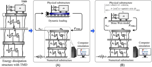
Taking the TLD damping structure as an example, in the RTHS, the main structure is numerically modeled and solved, and the TLD with strong nonlinearity is physically loaded. The dynamic response of the structure and the reaction of the TLD interact online in real time, and the architecture of RTHS is shown in Figure 1.

Details are in the caption following the image — **Figure 1**
Open in figure viewer PowerPoint

The real-time hybrid simulation system for tuned liquid damper (TLD) damping structure.

In Figure 1, M, C, and K are the mass matrix, damping matrix, and stiffness matrix of the structure. x,

\dot{{\boldsymbol{x}}}

, and

\ddot{{\boldsymbol{x}}}

are the displacement, velocity, and acceleration vectors of the structure.

{\ddot{{x}}}_{{g}}

is the earthquake acceleration. F_TLD is the TLD reaction. Equation (1) is the dynamic equation of the main structure

[M]\{\ddot{{x}}\}+[C]\{\dot{{x}}\}+[K]\{x\}=-[M]{\ddot{{x}}}_{g}+{F}_{\mathrm{TLD}}

()

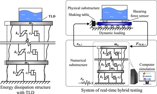
The RTHS can apply a larger TLD model to avoid overestimating the shock absorption performance of TLD due to the size effect.²⁴

2.1 Offline global iteration strategy

Load the physical substructure in advance, then use strong nonlinear fitting techniques such as NNs to accurately model it, and finally complete the offline simulation of the numerical substructure and the physical substructure constitutive model. In the above process, the numerical solution and the loading equipment no longer interact in real time. Since there is no real-time numerical solution requirement, a larger, more refined and nonlinear numerical substructure can be further adopted. Therefore, the RTHS shown in Figure 1 can be realized through the offline hybrid simulation shown in Figure 2.

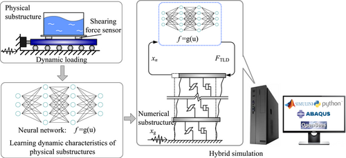
In particular, it is pointed out that the modeling of the physical substructure by NNs should be based on a large-scale data set, that is, a large number of preload tests on the physical substructure, so the offline hybrid simulation method is suitable for conditions in which the physical substructure is nondestructive. The data set is established by using the measured loading state of the loading device and the response of the physical substructure. The agent model trained is the mapping relationship between the actual load and dynamic response of the structure, which avoids the influence of the amplitude and phase errors of the loading device on RTHS.

There are general finite element software OpenSEES, ABAQUS, ANSYS, and so forth, and structural design finite element software SAP2000, ETABS, MIDAS, and so forth. Among the above six software, only OpenSEES can interact with the external models step by step, which makes it difficult to apply many large-scale, complex boundary, and nonlinear numerical models to hybrid experiments.

To solve the above problem, this study proposed an offline global iteration strategy to complete the interface interaction between numerical and physical substructures. Based on the fixed point iteration (FPI) algorithm,²⁵ the iteration process is shown in Figure 3. At the beginning of the iteration, input external excitation time history x_g into the numerical substructure, and calculate the initial state of the structure and interface response time history x₀. Then, input interface response time history x₀ into the physical substructure (NN agent model), and obtain its reaction time history F₀. Then, calculate the response of the structure to external excitation x_g and interface reaction F₀ again, and obtain a new structural state, at this point the first iteration has been complete. Every iteration can be completed with the following steps:

1.
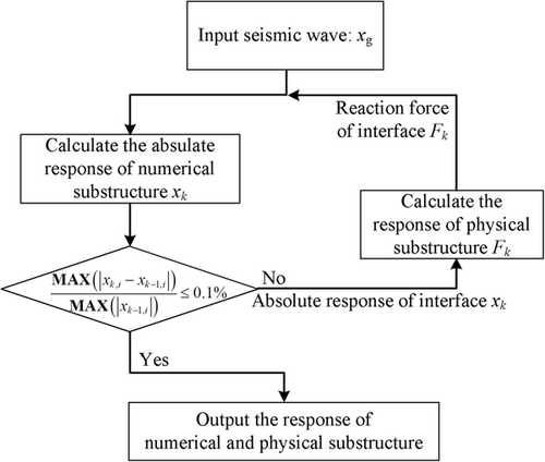
Input the interface displacement time history x_k−1 for the physical substructure, and calculate the interface reaction F_k, where k is the current iteration number.
2.
Input the external excitation time history x_g and the new interface reaction time history F_k for the numerical substructure, and update the structural dynamic time history response x_k.

The above iterative process can be represented by Equation (2), where k is the current iteration number.
${x}_{k}=I({x}_{k-1}),\unicode{x02007}\unicode{x02007}k=1,2,3,\text{\unicode{x02026}}$ ()
3.
If x* exists to make Equation (3) valid, then the FPI algorithm converges, and x* is the solution of the formula, otherwise the iteration divergence.

\mathop{\mathrm{lim}}\limits_{l\to \infty }{x}_{l}={x}^{* }

()

The convergence is judged according to the interface state of the two adjacent times. The convergence condition is shown in Equation (4), where k represents the current iteration number, i represents a step in the time history, and n is the total number of discrete steps.

\frac{\mathrm{MAX}(| {x}_{k,i}-{x}_{k-1,i}| )}{\mathrm{MAX}(| {x}_{k-1,i}| )}\le 0.001,\unicode{x02007}i=1,2,3,\text{\unicode{x02026}},n

()

2.2 Time-series modeling method of LSTM NN

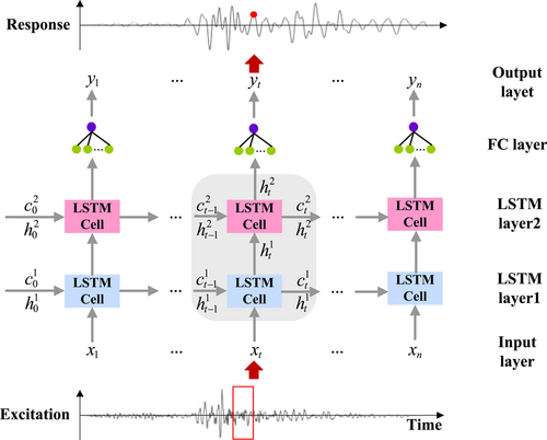
The multilayer LSTM NN is used to model and predict the nonlinear dynamic response of the physical substructure, and its topology is shown in Figure 4. LSTM NN is improved from recurrent NN (RNN). It was first proposed by Hochreiter and Schmidhuber²⁶ in 1997 to deal with the disappearance of gradients in RNN training and to learn the long-term dependence of data.²⁷ LSTM NN is a chain recursive structure with repetitive modules. Through the construction form of a multilayer stack, the nonlinear law representation ability of the model can be effectively improved. The model inputs the time-series data into the first LSTM layer and then takes the output of the first layer as the input of the second layer, and so on. After the last LSTM layer, the linear layer is used to integrate the high-dimensional information data output from the LSTM layer into the final prediction result of the model. LSTM neural network realizes autoregression by transmitting unit state and hidden state, and its time history prediction process is similar to the time-domain step-by-step integration method.

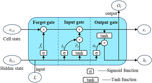
Each LSTM unit includes structures such as an input gate, a forget gate, an output gate, and a memory unit, as shown in Figure 5. Among them, the input gate controls whether the current input information is updated to the LSTM, the forget gate controls whether the memory before the current moment needs to be forgotten, and the output gate controls whether the current memory is used for output. These gating mechanisms enable LSTM to represent the timing dependence better.

In Figure 5, the calculation of the forget gate can be represented by Equation (5), the calculation of the input gate can be represented by Equation (6), the calculation of the cell state can be represented by Equation (7), and the calculation of the output and hidden state in the output gate can be represented by Equation (8)

{f}_{t}=\sigma ({{\rm{W}}}_{f}\cdot [{h}_{t-1},{I}_{t}]+{b}_{f})

()

\begin{array}{ccc}{i}_{t} & = & \sigma ({W}_{i}\cdot [{h}_{t-1},{I}_{t}]+{b}_{i})\\ {\mathop{c}\limits^{\unicode{x0007E}}}_{t} & = & \tanh ({W}_{c}\cdot [{h}_{t-1},{I}_{t}]+{b}_{c})\end{array}

()

{c}_{t}={f}_{t}\ast {c}_{t-1}+{i}_{t}\ast {\tilde{c}}_{t}

()

\begin{array}{ccc}{o}_{t} & = & \sigma ({W}_{o}\cdot [{h}_{t-1},{I}_{t}]+{b}_{o})\\ {O}_{t} & = & {h}_{t}={o}_{t}\ast \tanh ({c}_{t})\end{array}

()

where W and b are weight matrix and bias vector. σ represents the Sigmoid activation function, and tanh represents the tanh activation function.

3 NUMERICAL VERIFICATION

The feasibility of the OIHS-NN method is verified by numerical simulation, taking the TMD damping structure as an example.

3.1 Numerical simulation of RTHS for TMD damping structures

As shown in Figure 6A, in RTHS the TMD is the physical substructure, and the main structure is the numerical substructure. Numerical simulation of RTHS is carried out, as shown in Figure 6B. The 9-layer benchmark model recommended by Ohtori et al.²⁸ was adopted as the numerical substructure. The mass and stiffness of each layer are shown in Table 1. The stiffness adopted in the bilinear model and the yield displacement of each layer are shown in Table 2. The stiffness reduction coefficient after yielding is 0.5. Rayleigh damping is used, and the damping ratio is 2%. The response of the main structure was solved by the Newmark-β method. The Bouc–Wen hysteretic model was adopted for the restoring force, which is composed of elastic restoring force and hysteretic restoring force. The nonlinear restoring force was obtained by solving Equation (9) differential equation using ODE4, and the acceleration, velocity, and displacement of the TMD SDOF (single degree of freedom) system were calculated by the central difference method. The parameters of TMD are shown in Table 3. The simulation step size was 10 ms, which is realized by Python programming.

\left\{\begin{array}{c}{f}_{k}(t)=\alpha ku(t)+(1-\alpha )kz(t){u}_{y}\\ \dot{z}(t)=\frac{A-{| z(t)| }^{j}(\gamma +\text{sgn}(\dot{u}(t)\cdot z(t))\cdot \beta )}{{u}_{y}}\dot{u}(t)\end{array}\right.

()

where f_k(t) is restoring force; u(t) is the displacement; z(t) is the internal hysteresis variable; k is the initial elastic stiffness; u_y is the yield displacement; α is the ratio of the stiffness after yielding to the initial stiffness; and A, γ, β, and j are the hysteresis parameters, which control the shape of the hysteresis loop and are dimensionless. The parameters of the TMD numerical model are shown in Table 3.

Table 1. Parameters of 9-layer benchmark structural interlayer shear model.

Layer	1	2	3	4	5	6	7	8	9
Mass 10⁵ (kg)	10.1	9.89	9.89	9.89	9.89	9.89	9.89	9.89	10.7
Stiffness 10⁸ (N/m)	3.1681	3.0604	2.8943	2.8060	2.7540	2.7008	2.6374	2.5824	2.5279

Table 2. Yield displacements of 9-layer benchmark structural interlayer shear model.

Layer	1	2	3	4	5	6	7	8	9
Yield displacement (m)	0.035	0.018	0.019	0.019	0.020	0.020	0.021	0.021	0.022

Table 3. Parameters of the TMD numerical model.

m_TMD (kg)	k (N/m)	ζ (%)	u_y (m)	A	γ	β	j	α
1.801 × 10⁵	1.255 × 10⁶	10.73	0.1	1	0.5	0.5	1.5	0.2

Abbreviation: TMD, tuned mass damper.

3.2 Accuracy verification of the LSTM model

To establish the neural network training data set, a total of 57 seismic waves were selected as TMD input excitations to calculate the reaction time history of TMD. The selected seismic waves and divisions of the NN train and test sets are shown in Table 4. The data in the test set did not participate in the error backpropagation process of model parameter optimization and was only used for testing the accuracy of the model.

Table 4. Selection and division of seismic wave.

Earthquake record	Duration (s)	Quantity	Division
East Japan	300	26	Train set
Imperial Valley	37.06–50.08	24	Test set
Coalinga	58.16	2
Whittier Narrows	40.00	2
Superstition Hills	29.85	2

To make the amplitude generalization ability of the NN model meet the application requirements of structural seismic response prediction, the input peak ground acceleration (PGA) was selected as 1, 5, and 9 m/s². The reaction time history under all the seismic waves was calculated, and the NN train and test sets were established.

To effectively improve the neural network's learning ability to the dynamic time-delay characteristics, multistep excitation was used to predict single-step responses. When the prediction method of multistep input and single-step output is used, to ensure the integrity of the prediction result, the zero-filling operation needs to be performed at the front end of the input sequence. Taking the input duration as 60 steps, the mapping relationship of the NN is shown in Equation (10)

{F}_{\text{TMD},t}=G({x}_{\text{abs},t-59},{x}_{\text{abs},t-58},\ldots ,{x}_{\text{abs},t},{\dot{x}}_{\text{abs},t-59},{\dot{x}}_{\text{abs},t-58},\ldots ,{\dot{x}}_{\text{abs},t},{\ddot{x}}_{\text{abs},t-59},{\ddot{x}}_{\text{abs},t-58},\ldots ,{\ddot{x}}_{\text{abs},t})

()

where F_TMD,t is predicted value of TMD reaction at step t. x_abs,t,

{\dot{{x}}}_{\mathrm{abs},{t}}

, and

{\ddot{{x}}}_{\mathrm{abs},{t}}

are, respectively, displacement, velocity, and acceleration of step t of the input sequence.

The OIHS-NN method does not require step-by-step interaction; thus, the LSTM model adopts a whole sequence prediction approach. The topology of the NN is shown in Table 5, where n represents the sequence length. The model consisted of two stacked LSTM layers and one linear integration layer, and the different layers were connected linearly. The data set was Z-score standardized before the model training. Mean-square error (MSE) loss function was used in NN training, as shown in Equation (11). The Adam optimization algorithm²⁹ was used to optimize the model parameters, and the dynamic learning rate was set to decrease along the reciprocal, as shown in Figure 7. The error in the model training decrease was shown in Figure 8, and the final MSE error tended to be flat, which determines that the LSTM model had trained completely. The above content was implemented through the Pytorch framework in Python code

\mathrm{MSE}=\frac{{\sum }_{1}^{n}{({Y}_{t}-{T}_{t})}^{2}}{n}

()

where Y_t is the tth element of the prediction sequence, T_t is the tth element of the target sequence, and n is the sequence length.

Table 5. Structure of LSTM neural network model.

Layer	Type	Input dimension	Output dimension
Input (LSTM1)	LSTM	n × (3 × 60)	n × 120
LSTM2	LSTM	n × 120	n × 60
Output	Linear	n × 60	n × 1

Abbreviation: LSTM, long-short time memory.

The peak error (PE) was used to evaluate the error at the peak point, as shown in Equation (12). The root mean relative square error (RMRSE) was used to evaluate the accuracy of the whole time history, as shown in Equation (13)

\text{PE}(y,\hat{y})=\left|\frac{{| \hat{y}| }_{\max }-{| y| }_{\max }}{{| y| }_{\max }}\right|\times 100 \%

()

\mathrm{RMRSE}=\sqrt{\frac{1}{n}\sum _{t=1}^{n}{\left(\frac{{\hat{y}}_{t}-{y}_{t}}{| {y}_{t}| +\alpha {| y| }_{\max }}\right)}^{2}}

()

where |y|_max is the maximum absolute value of the true value, |

\hat{y}

|_max is the maximum absolute value predicted by the neural network, y_t is the true value of step t, and

{\hat{y}}_{t}

is the prediction of step t. The parameter α was introduced in Equation (13) to avoid the explosive growth of RMRSE, which was caused by the phase error when y_t approaches 0, and it was taken as 0.2.

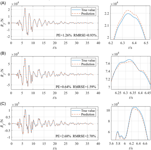
Taking the Imperial Valley earthquake input as an example, the time history prediction of TMD reaction under different amplitude excitations is shown in Figure 9.

3.3 Convergence verification of OIHS-NN

The convergence of the offline iterative hybrid simulation method was verified. For this structure, the iterative process is shown in Figure 10.

Where F_th,k is the TMD reaction time history of the kth iteration, x_th,k is the absolute response time history of the structure at the kth iteration, and x_g is the earthquake time history. The convergence criterion is shown in Equation (4). During the iterative process, the numerical substructure always satisfies Equation (14). For each iteration, the structural response time history x,

\dot{x}

\ddot{x}

and the TMD reaction F_TMD are all updated

[M]\{\ddot{x}\}+[C]\{\dot{{x}}\}+[K]\{x\}=-[M]{\ddot{{x}}}_{{g}}+{F}_{\text{TMD}}\{i\}

()

where {i} is a unit vector, indicating the position of TMD.

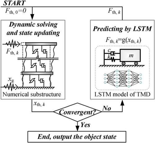
Input the Imperial Valley wave, and PGA = 4 m/s². It has converged after 40 times of iteration, and the comparison between the iteration results and the RTHS numerical simulation results is shown in Figure 11.

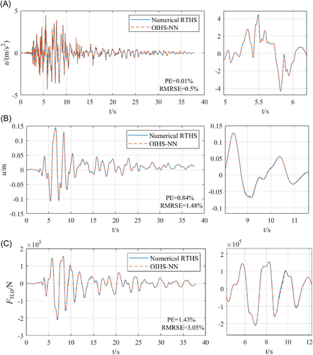
The results show that the LSTM NN has a strong fitting ability for nonlinear physical substructures, and the prediction PE and RMRSE are within 2.7%. The OIHS-NN method based on the FPI method converged after 40 iterations, and the errors of the structural response and TMD reaction time history of the overall structure is within 3.05%. The OIHS-NN can effectively converge and has high precision.

The analysis on the convergence behavior and accuracy of the OIHS-NN method with various PGAs was conducted. The 30 seismic records in the test set was employed for this purpose. The convergence condition count and the average iteration count for different PGAs are depicted in Figure 12, as well as the corresponding errors.

At lower PGAs, the OIHS-NN method necessitates a higher number of iterations, and in some cases may be even divergent. As the PGA gradually extends within the range of the training data set, OIHS-NN achieves stable convergence, and the iteration count diminishes with increasing PGA values. Furthermore, with the amplification of PGA, the convergence error also enlarges. Hence, to ensure the convergence and precision of OIHS-NN, it is necessary to appropriately select the PGAs of train set in accordance with the experimental objectives.

4 EXPERIMENTAL VERIFICATION

RTHS was used to verify the convergence and accuracy of the OIHS-NN method. The TLD damping structure was taken as an example, the RTHS system is shown in Figure 1. First, the RTHS of the TLD damping was carried out, and then the data set was established based on the table excitation and the TLD reaction. The LSTM model was trained and compared with the test results and the calculation results of the classical simplified model. Finally, OIHS-NN was carried out, and compared with the RTHS results and the numerical simulation results of the simplified model.

4.1 RTHS of TLD damping structures

As shown in Figure 13, the physical substructure TLD was loaded using a shaking table. The length of the TLD model along the seismic excitation direction was 2.1 m, the width was 2 m, and the static water level was 0.36 m. The numerical substructure adopted the 9-layer benchmark model. The parameters are shown in Tables 1 and 2. Rayleigh damping is adopted, the damping ratio is 5%, and the yield factor of stiffness is 0.1. The number of TLDs on the main structure was changed to control the mass ratio of TLDs to the main structure. The time step in the RTHS was 1 ms, and the real-time hybrid test architecture is shown in Figure 14. In the test, the reaction of the physical substructure was only the reaction of water, which was, the reaction of the numerical substructure was the shear force measured by the sensor minus the inertial force of the empty tank and the connecting steel plate, which is shown in Equation (15)

{F}_{\text{TLD}}={F}_{{\rm{t}}}-{a}_{{\rm{t}}}({m}_{{\rm{b}}}+{m}_{{\rm{T}}})

()

where F_t represents the reaction force measured by the shear stress sensor, a_t corresponds to the acceleration sensor's test reading on the steel plate, m_b signifies the mass of the steel plate, and m_t denotes the mass of the empty tank.

In this system, the signal sent to the controller was the absolute displacement, and the absolute displacement was taken as the variable. The dynamic equation of the structure is shown in Equation (16). The velocity is obtained by integrating on both sides of the equation, and the displacement is obtained by integrating again. Therefore, the absolute displacement, velocity, and acceleration response of the structure can be obtained by integrating twice, which is realized in Simulink software

[M]{\ddot{{x}}}_{\text{abs}}=-[K]({{x}}_{\text{abs}}-{{x}}_{{g}})-[C]({\dot{{x}}}_{\text{abs}}-{\dot{x}}_{g})+{n}_{t}{F}_{\text{TLD}}\{i\}

()

where [M], [C], and [K] is matrix of mass, damping, and stiffness of the main structure;

{{x}}_{\text{abs}}

{\dot{{x}}}_{\text{abs}}

, and

{\ddot{{x}}}_{\text{abs}}

are absolute displacement, velocity, and acceleration vectors of the structure;

{x}_{{g}}

and

{\dot{x}}_{{g}}

are earthquake displacement and velocity; F_TLD is the reaction of one TLD; n_t is the number of TLD units; {i} is unit vector, indicating the position of TLD.

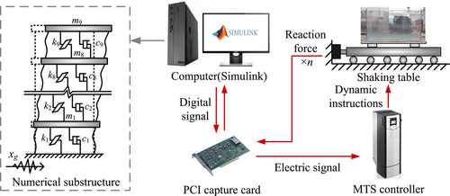
Considering the limitation of the loading displacement of the shaking table, to make the structure enter a nonlinear state, the critical yield displacement was reduced in different conditions. The variables controlled in the RTHS included seismic wave, PGA, mass ratio, and critical yield displacement reduction coefficient. The statistics of working conditions are shown in Table 6.

Table 6. RTHS conditions of TLD damping structure.

Seismic wave	PGA (m/s²)	Mass ratio μ (%)	Discount of yield displacement β	Quantity
El-Centro	0.3–1.2	0.5–6	0.2–0.5/−	20
Kobe	0.3–2.5	0.5–6	0.2–0.5/−	30
Northridge	0.3–2	0.5–6	0.2–0.5/−	18
Hachinohe	0.3–0.6	0.5–6	0.2–0.5/−	9

Abbreviations: PGA, peak ground acceleration; RTHS, real-time hybrid simulation; TLD, tuned liquid damper.

4.2 Accuracy verification of the LSTM model

The input features of the LSTM model were excitation acceleration, velocity, and displacement, and the output feature was the reaction of TLD. The acceleration and displacement were measured by the sensors arranged on the connecting steel plate, and the velocity was obtained by the central difference method from displacement. The reaction was obtained by the shear force measured by the shear sensor minus the inertial force of the water tank and the connecting steel plate. The training samples of the LSTM model were divided into a train set and a test set. The six conditions in the test set were shown in Table 7, and the others were included in the train set. The data in the test set did not participate in the error backpropagation of parameter optimization, which was only used for testing LSTM model accuracy.

Table 7. Conditions in the test set.

Condition	Seismic wave	PGA (m/s²)	Mass ratio μ (%)	Discount of yield displacement β
1	El-Centro	0.8	3.5	0.3
2	Kobe	0.4	1.5	-
3	Kobe	0.4	0.5	0.2
4	Kobe	2	1.5	0.3
5	Northridge	0.8	1.5	0.3
6	Hachinohe	0.5	1.5	0.2

Abbreviation: PGA, peak ground acceleration.

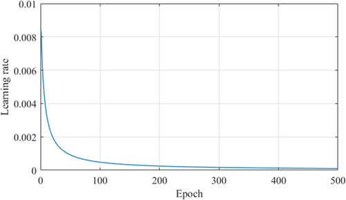
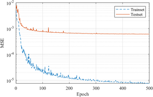
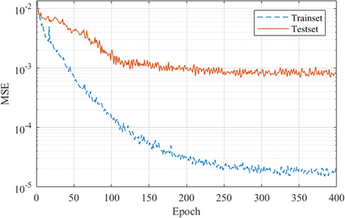
To increase the amount of spatiotemporal information contained in each step in the training data, the test data with the original step length of 1 ms was downsampled to 20 ms. The dynamic response of TLD has a certain time lag, and to effectively describe this characteristic, the time window size was selected as 240, which is about twice the basic period of TLD. The structure of the LSTM model is shown in Table 8, where n represents the sequence length. In the training process, the dynamic learning rate with reciprocal decline was adopted, as shown in Figure 15. The decrease of MSE during training is shown in Figure 16. The above content was realized through the Pytorch framework in Python code.

Table 8. The structure of the LSTM neural network model.

Layer	Type	Input dimension	Output dimension
Input (LSTM1)	LSTM	n × (3 × 240)	n × 240
LSTM2	LSTM	n × 240	n × 120
Output	Linear	n × 120	n

Abbreviation: LSTM, long-short time memory.

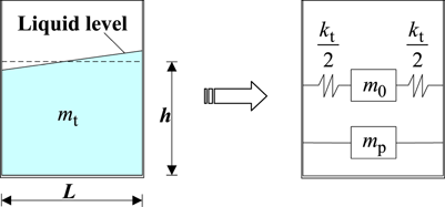
At the same time, the LSTM model was also compared with the TLD lumped mass model to verify the prediction accuracy. The TLD lumped mass model was proposed by Housner³⁰ in 1957. It assumes that the liquid is incompressible and nonviscous, without rotation, and without wave breakage. The hydrodynamic pressure is divided into two parts, one part is the pulsating mass that generates pulsating pressure, and the other part is simplified as the oscillating mass elastically connected to the tank, which generates oscillating pressure, as shown in Figure 17.

Where the oscillating mass m₀, pulsating mass m_p, and spring stiffness k_t are calculated by Equation (17)

\begin{array}{c}{m}_{{\rm{p}}}={m}_{t}\frac{\tanh (1.7L/2h)}{1.7L/2h}\\ {m}_{0}={m}_{t}\frac{0.83\,\tanh (1.6\times 2h/L)}{1.6\times 2h/L}\\ {k}_{t}=\frac{3{{m}_{0}}^{2}gh}{{m}_{t}{(L/2)}^{2}}\end{array}

()

where L is the length of the water tank in the excitation direction, h is the depth of water, m_t is the mass of water, and g is the gravitational acceleration.

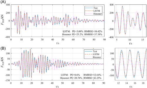
Comparing the calculation accuracy of the LSTM model and the lumped mass model, the time history of the TLD reaction is shown in Figure 18. For each working condition in the test set, the error of the LSTM model and the lumped mass model are shown in Table 9.

Table 9. Accuracy of LSTM prediction and Housner model result.

Condition	PE	RMRSE	PE	RMRSE
	LSTM		Housner
1	5.08	10.42	25.92	37.38
2	4.32	16.1	38.72	40.7
3	1.89	10.16	52	51.76
4	0.6	12.64	20.76	42.25
5	5.16	9.32	7.34	78.56
6	4.55	10.89	12.44	63.59

Abbreviations: PE, peak error; RMRSE, root mean relative square error.

From Table 9, the LSTM model exhibits a stronger nonlinear representation ability for the TLD reaction. Its time history prediction PE is up to 5.16%, and RMRSE is up to 16.1%. The prediction accuracy of each working condition is significantly higher than that of the lumped mass model.

4.3 Convergence verification of OIHS-NN

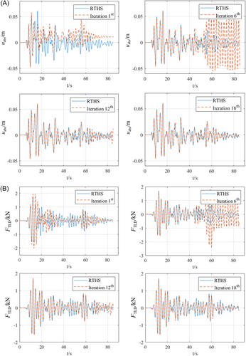
The convergence and accuracy of the OIHS-NN method were verified. For the TLD damping structure, the iterative process is shown in Figure 19.

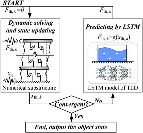
Where F_th,k is the TLD reaction time history of the kth iteration; x_th,k is the absolute structural response time history of the k_th iteration, x_g is the earthquake time history, and the convergence criterion is shown in Equation (4). In the iterative process, the numerical substructure always satisfies Equation (16). In each iteration, the structural response time history ${x}_{\text{abs}}$ , ${\dot{x}}_{\text{abs}}$ , ${\ddot{{x}}}_{\text{abs}}$ , and the TLD reaction F_TLD would be updated.

Taking test condition 1 as an example, the iterative process is shown in Figure 20. The test condition 1 took 24 iterations to converge. The iterative convergence results are shown in Figure 21, and are compared with the results of RTHS and the Housner model numerical simulation. The displacement and acceleration of the top layer of the structure and the reaction force of TLD all meet PE ≤ 2% and RMRSE ≤ 20%, which is significantly more accurate than the numerical simulation based on the simplified model of TLD.

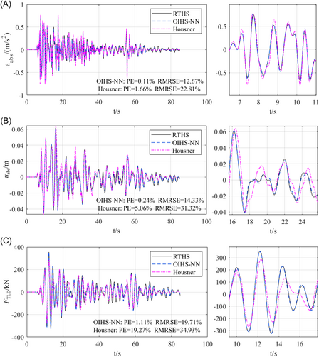
After a finite number of iterations, all the test conditions converged. The statistics of convergence speed and accuracy of each test condition are shown in Table 10.

Table 10. Convergence rate and iteration precision statistics of OIHS-NN.

Condition	Times of iteration	Acceleration		Displacement		F_TLD
Condition	Times of iteration	PE	RMRSE	PE	RMRSE	PE	RMRSE
1	24	0.11	12.67	0.24	14.33	1.11	19.60
2	25	3.22	7.61	2.96	21.73	27.15	32.62
3	9	1.72	2.18	2.09	4.00	2.71	13.37
4	14	7.85	7.37	1.91	10.20	0.06	20.73
5	19	0.29	11.09	0.27	12.78	5.75	17.45
6	19	2.75	12.08	1.10	8.94	0.36	14.99

Abbreviations: PE, peak error; RMRSE, root mean relative square error; TLD, tuned liquid damper.

In this chapter, the convergence and accuracy of the OIHS-NN method were verified by comparing it with the RTHS of the TLD damping structure. The test results show that the LSTM model has a strong fitting ability for the nonlinear physical substructure, and the predicted PE and RMRSE are within 2.7%, which is obviously superior to the accuracy of the simplified mechanical model. The OIHS-NN method can converge after a finite number of iterations, and has high accuracy. The PE of the structure response is within 8%, which has obvious advantages over the numerical simulation of the simplified model. However, it can also be found that some conditions had dependence on seismic waves, and the law and reason for this influence need to be further studied.

5 CONCLUSIONS

This paper proposes an OIHS-NN. The method does not require the computer to solve the numerical substructure in real time nor does it require the interaction step-by-step between the numerical substructure and the physical substructure, which expanded the application of large-scale, nonlinear, and refined finite element models in hybrid simulation. Taking the tuned damping structure as examples, numerical simulation and experimental verification of this method are carried out, and the conclusions are as follows:

1.
The LSTM neural network model is used to predict the TMD reaction force with Bouc–Wen hysteresis, and its PE ≤ 2.68%. The model was also used to predict the TLD reaction with significant nonlinearity, and its PE ≤ 5.16%. The LSTM model's accuracy is significantly better than the simplified mechanical model, whose PE is 38.72%. The prediction accuracy of the neural network for the nonlinear dynamic response of the structure is high, and its nonlinear representation ability is much higher than that of the simplified mechanical model.
2.
It is verified by experiment that even if the physical substructure has strong nonlinearity such as the TLD, the OIHS-NN method could still converge within 25 iterations, the convergence met application requirements.
3.
The PE of structure response time history obtained by OIHS-NN method was less than 7.85%. Individual working conditions had dependence on the input excitation, whose error is slightly larger. Overall, OIHS-NN has much better accuracy than the numerical simulation of the simplified model. It is feasible to use this method for hybrid simulation.

In the follow-up work, the errors and convergence influencing factors of the OIHS-NN method need to be further studied, and the iterative algorithm will be improved to reduce the iteration time.

ACKNOWLEDGMENTS

The authors gratefully acknowledge the support of the National Natural Science Foundation of China (51978016) in the pursuance of this work.

CONFLICTS OF INTEREST

The authors declare no conflicts of interest.

REFERENCES

1Hakuno M, Shidawara M, Hara T. Dynamic destructive test of a cantilever beam, controlled by an analog-computer. Proc Jpn Soc Civ Eng. 1969; 1969(171): 1-9.
10.2208/jscej1969.1969.171_1
Google Scholar
2Nakashima M, Kato H, Takaoka E. Development of real-time pseudo dynamic testing. Earthq Eng Struct Dyn. 1992; 21(1): 79-92.
10.1002/eqe.4290210106
Web of Science® Google Scholar
3Horiuchi T, Inoue M, Konno T, Namita Y. Real-time hybrid experimental system with actuator delay compensation and its application to a piping system with energy absorber. Earthq Eng Struct Dyn. 1999; 28(10): 1121-1141.
10.1002/(SICI)1096-9845(199910)28:10<1121::AID-EQE858>3.0.CO;2-O
Web of Science® Google Scholar
4Horiuchi T, Konno T. A new method for compensating actuator delay in real-time hybrid experiments. Philos Trans R Soc Lond Ser A. 2001; 359(1786): 1893-1909.
10.1098/rsta.2001.0878
Web of Science® Google Scholar
5Darby AP, Williams MS, Blakeborough A. Stability and delay compensation for real-time substructure testing. J Eng Mech. 2002; 128(12): 1276-1284.
10.1061/(ASCE)0733-9399(2002)128:12(1276)
Web of Science® Google Scholar
6Ahmadizadeh M, Mosqueda G, Reinhorn AM. Compensation of actuator delay and dynamics for real-time hybrid structural simulation. Earthq Eng Struct Dyn. 2008; 37(1): 21-42.
10.1002/eqe.743
Web of Science® Google Scholar
7Chae Y, Kazemibidokhti K, Ricles JM. Adaptive time series compensator for delay compensation of servo-hydraulic actuator systems for real-time hybrid simulation. Earthq Eng Struct Dyn. 2013; 42(11): 1697-1715.
10.1002/eqe.2294
Web of Science® Google Scholar
8Carrion JE, Spencer BF, Phillips BM. Real-time hybrid simulation for structural control performance assessment. Earthq Eng Eng Vib. 2009; 8(4): 481-492.
10.1007/s11803-009-9122-4
Web of Science® Google Scholar
9Tang Z, Dietz M, Hong Y, Li Z. Performance extension of shaking table-based real-time dynamic hybrid testing through full state control via simulation. Struct Control Health Monit. 2020; 27(10):e2611.
10.1002/stc.2611
Web of Science® Google Scholar
10Wang M, Au FTK. Assessment and improvement of precise time step integration method. Comput Struct. 2006; 84(12): 779-786.
10.1016/j.compstruc.2006.02.001
Web of Science® Google Scholar
11Zhu F, Wang JT, Jin F, Gui Y. Comparison of explicit integration algorithms for real-time hybrid simulation. Bull Earthq Eng. 2016; 14(1): 89-114.
10.1007/s10518-015-9816-0
Web of Science® Google Scholar
12Chang SY. A new family of explicit methods for linear structural dynamics. Comput Struct. 2010; 88(11): 755-772.
10.1016/j.compstruc.2010.03.002
Web of Science® Google Scholar
13Kolay C, Ricles JM. Development of a family of unconditionally stable explicit direct integration algorithms with controllable numerical energy dissipation. Earthq Eng Struct Dyn. 2014; 43(9): 1361-1380.
10.1002/eqe.2401
Web of Science® Google Scholar
14Gui Y, Wang JT, Jin F, Chen C, Zhou MX. Development of a family of explicit algorithms for structural dynamics with unconditional stability. Nonlinear Dyn. 2014; 77(4): 1157-1170.
10.1007/s11071-014-1368-3
Web of Science® Google Scholar
15Tang Z, Dong X, Li Z, et al. Implementation of real-time hybrid simulation based on GPU computing. Struct Des Tall Spec. 2022; 31(12):e1942.
10.1002/tal.1942
Web of Science® Google Scholar
16Zhu F, Wang JT, Jin F, Chi FD, Gui Y. Stability analysis of MDOF real-time dynamic hybrid testing systems using the discrete-time root locus technique. Earthq Eng Struct Dyn. 2015; 44(2): 221-241.
10.1002/eqe.2467
Web of Science® Google Scholar
17Zhang R, Liu Y, Sun H. Physics-informed multi-LSTM networks for metamodeling of nonlinear structures. Comput Methods Appl Mech Eng. 2020; 369:113226.
10.1016/j.cma.2020.113226
Web of Science® Google Scholar
18Xu Z, Chen J, Shen J, Xiang M. Recursive long short-term memory network for predicting nonlinear structural seismic response. Eng Struct. 2022; 250:113406.
10.1016/j.engstruct.2021.113406
Web of Science® Google Scholar
19Han X, Feng R, Ji J, et al. Research on parameters of the RC beam lumped plastic hinge model based on deep learning. Eng Mech. 2021; 38(11): 160-169.
Google Scholar
20Bas EE, Moustafa MA. Communication development and verification for Python-based machine learning models for real-time hybrid simulation. Front Built Environ. 2020; 6:574965.
10.3389/fbuil.2020.574965
Google Scholar
21Bas EE, Moustafa MA. Performance and limitations of real-time hybrid simulation with nonlinear computational substructures. Exp Tech. 2020; 44(6): 715-734.
10.1007/s40799-020-00385-6
Web of Science® Google Scholar
22Chen C, Yang Y, Hou H, Peng C, Xu W. Real-time hybrid simulation with multi-fidelity Co-Kriging for global response prediction under structural uncertainties. Earthq Eng Struct Dyn. 2022; 51(11): 2591-2609.
10.1002/eqe.3690
Web of Science® Google Scholar
23Tang Z, Gao F, Liu H, Li Y. Implementation of shaking table based offline hybrid testing through neural networks. Structures. 2023; 48: 21-30.
10.1016/j.istruc.2022.12.050
Web of Science® Google Scholar
24Zhu F, Wang JT, Jin F, Lu LQ, Gui Y, Zhou MX. Real-time hybrid simulation of the size effect of tuned liquid dampers. Struct Control Health Monit. 2017; 24(9):e1962.
10.1002/stc.1962
Web of Science® Google Scholar
25Amann H. Fixed point equations and nonlinear eigenvalue problems in ordered Banach spaces. SIAM Rev. 1976; 18(4): 620-709.
10.1137/1018114
Web of Science® Google Scholar
26Hochreiter S, Schmidhuber J. LSTM can solve hard long time lag problems. Adv Neural Inf Process Syst. 1996; 9: 473-479.
Google Scholar
27Bengio Y, Simard P, Frasconi P. Learning long-term dependencies with gradient descent is difficult. IEEE Trans Neural Netw. 1994; 5(2): 157-166.
10.1109/72.279181
CAS PubMed Web of Science® Google Scholar
28Ohtori Y, Christenson RE, Spencer BF, Dyke SJ. Benchmark control problems for seismically excited nonlinear buildings. J Eng Mech. 2004; 130(4): 366-385.
10.1061/(ASCE)0733-9399(2004)130:4(366)
Web of Science® Google Scholar
29Kingma DP, Ba J. Adam: a method for stochastic optimization. Int Conf Learn Represent. 2015; 5: 6.
Google Scholar
30Housner GW. Dynamic pressures on accelerated fluid containers. Bull Seismol Soc Am. 1957; 47(1): 15-35.
10.1785/BSSA0470010015
Google Scholar

Volume2, Issue4

December 2023

Pages 383-402

This article also appears in:

Earthquake engineering simulation through shaking table tests

Implementation of offline iterative hybrid simulation based on neural networks

Abstract

1 INTRODUCTION