Probabilistic seismic performance of pylons of a cable-stayed bridge under near-fault and far-fault ground motions
Abstract
Pulse-like ground motions significantly influence structural responses, indicating that more consideration should be given to the seismic design of structures in the near-site region. However, less effort focuses on the seismic response of a cable-stayed bridge under near-field pulse-like excitations, and the difference in structural responses caused by near-field pulse-like and far-field ground motions is not fully captured. This paper, therefore, aims to investigate the effect of pulse-like ground motions on a cable-stayed bridge, and it presents a comparison of far-field earthquakes. Considering the finite number of recorded ground motions, artificial pulse-like ground motions are adopted in this study. Furthermore, two classical intensity measures (peak ground velocity [PGV] and peak ground acceleration) were used to establish the probabilistic seismic demand model for cable-stayed bridges. Then, fragility curves associated with the pylon of the bridge were compared under the action of different types of excitations, and the damage state of the whole pylon is presented through the median point of the slight damage of the curvature of each pylon section. The results indicate that the bottom section of the pylon is damaged first under different seismic excitations, with the PGV as the index. Moreover, far-fault ground motions have a greater impact on the curvature response of the longitudinal bridge section of the pylon than the near-fault ground motions, so the damage is more serious.
1 INTRODUCTION
- (1)
The propagation direction of a fault is the main influencing factor of near-site vibrations, but the soil condition has little influence. For far-field records, the soil condition is the most important for wave propagation and site conditions.
- (2)
In the near-field region, there is an obvious low-frequency jump in the earthquake's acceleration time-history curves and a continuous jump in the time history of velocity and displacement, and the duration of ground motions is very short. The time history of acceleration, velocity, and displacement displayed by far-field records have cyclic motions and last for a long time.
- (3)
The near-field ground motion speed is very large. In the Beijing and Kobe earthquakes, the ground peak velocity was relatively large, that is, 150–200 cm/s, while in the far-field region, the velocity did not exceed 30–40 cm/s. Therefore, in the near-field design concept, velocity is the most important, replacing the most important acceleration in the far field.
- (4)
Due to the consistency between the ground vertical motion frequency and structure vertical frequency, an important vertical plane amplification effect may occur. At the same time, considering that the probability of plastic deformation and attenuation in the vertical displacement direction decreases, the behavior in the vertical direction may be the most important to the structure in the near-field region.
- (5)
For the jumping characteristics of ground motions and high speed, the demand for structure ductility may be very high. Moreover, the short period of ground motions is a very favorable factor in the near-field region. Hence, the balance among the ductile demand, jumping behavior, and short duration must be reasonably analyzed.
Compared with far-fault earthquakes, near-fault earthquakes have three main features of ground motions: directional effect, velocity pulse-like effect, and vertical acceleration effect.4, 5 In some earthquakes, the rupture velocity of faults is close to the shear speed of the soil layer, resulting in the superposition of waves caused by the fault fracture and earthquake propagation in the soil layer, forming pulse-like earthquakes. The superposition of a fault rupture wave and earthquake energy in seismic causes an energy surge, which leads to the emergence of a velocity pulse. Sucuoǧlu and Nurtuǧ6 quantified the velocity pulse effect by utilizing the ratio of the peak ground acceleration (PGA) to peak ground velocity (PGV). The amplitude of the vertical component of ground motions recorded in some near-field areas is also large, even close to the amplitude of the horizontal component, and contains a large number of high-frequency components. This phenomenon is called the vertical acceleration effect. This effect has a serious impact on flexible structures, such as bridges, long-span structures, and long cantilever structures.
At present, there are few studies on the analysis and comparison of the response law and fragility of cable-stayed bridges under near-field and far-field earthquakes in China. In probabilistic seismic hazard analysis, traditional seismic models do not consider the pulse effect of ground motions on bridge structures, which would underestimate the hazard of bridges near faults. Using a cable-stayed bridge as an example, Zhong et al.7 propose a reliable risk assessment tool for large-span bridges with spatially varying ground motions. Yang et al.8 chose Taiwan(China)'s lumped near-fault ground motion records as the ground motion input and systematically investigated the influence of near-fault ground motions' directional effect, velocity pulse-like effect, and vertical acceleration effect on the earthquake's response to bilinear single-degree-of-freedom system, long-period isolated buildings, and cable-stayed bridges. Fu9 studied the seismic performance of a curved continuous beam bridge considering collisions under near-field and far-field seismic and found that the damage and failure of curved bridges will be more serious than those of far-field earthquakes. Zhang et al.10 used the Sutong Yangtze Bridge to analyze and study the seismic response of a large cable-stayed bridge under pulse-like ground motions. Their research results can provide a reference for the seismic design of large cable-stayed bridges under pulse-like ground motions. Zhang and Zhang11 studied the response of reinforced concrete rigid frame bridges under the longitudinal excitation of near-field and far-field ground motions using near-field and far-field vibrations recorded by four stations and put forward some suggestions on the seismic design of large rigid frame bridges located in some near-field areas.
Although the seismic performance of building structures located in near-field earthquakes has been widely studied for many years, there is little research on the response law and fragility of each section of the pylons of large cable-stayed bridges under pulse-like and far-fault earthquakes. Accordingly, the purpose of this paper is to select an optimal intensity measure (IM) and draw the probabilistic seismic demand model (PSDM) and fragility curve of the pylon columns of bridges under the action of near-field pulse-like and far-field earthquakes. Finally, the PGA and PGV are selected as the strength indices to analyze and compare the curvature response law (along the bridge direction) and fragility of each section of the main pylon of a huge cable-stayed bridge under the action of near-field and far-field earthquakes. These results will provide a reference for the seismic demand estimation of cable-stayed bridges under near-field and far-field earthquakes.
2 GROUND MOTIONS
2.1 Artificial pulse-like ground motions
Although recorded seismic data are increasing, the records of near-fault motions, especially pulse ground motions, are still pretty scarce. The extensive destruction of engineering structures has prompted seismic engineers and seismologists to seek a deeper understanding of near-fault pulse ground motions. At the same time, the availability and convenience of near-fault ground motions data facilitate the study of such ground motions and their impact on structures.
Accordingly, the methodology of generating artificial pulse-like ground motion is used in this study. Ground motions are rotated and classified as pulse or nonpulse.
In this way, seven physical-related arguments (Ia, D5–95, D0–5, D0–30, , , and ) are used to perfectly define the course of showing the broadband near-field ground motion acceleration.
| Pulse parameters | Vp (cm/s) | Tp (s) | γ | ν/π (rad) | tmax,p (s) | ||
| Residual parameters | Ia,res (cm/s) | D5–95,res (s) | D0–5,res (s) | D0–30,res (s) | fmid,res (Hz) | ζf,res | |
| Orthogonal parameters | Ia,PO (cm/s) | D5–95,PO (s) | D0–5,PO (s) | D0–30,PO (s) | fmid,PO (Hz) | fPO (Hz/s) | ζf,PO |
2.2 Selection of far-fault ground motions
This study selected far-fault records used in Jiang et al.14 Records 1–80 were selected from the Pacific Earth Engineering Research Center (PEER), and records 80–100 were selected from the database of the SAC project. The magnitude ranges from 5.8 to 6.9, and the epicentral distance ranges from 10 to 60 km. The PGA, magnitude, and epicentral distance of the records are shown in Appendix Table A1. The 20 ground motions selected from the SAC have exceedance probabilities of 2% and 10% in 50 years. The corresponding acceleration spectrum is given in Figure 1B.

2.3 Input ground motions
To obtain the desired seismic effects, 100 far-field records and 121 artificial pulse-like ground motions were inputted along the longitudinal bridge section, transversal bridge section, and vertical bridge section, and the critical elements of the cable-stayed bridge were analyzed through dynamic time-history analysis.
3 CASE STUDY
3.1 Modeling of the bridge
A single-tower, double-cable-plane cable-stayed bridge was taken as the study object. Its span combination is 150 + 150 m. The general size layout of the bridge is presented in Figure 2. The detailed geometric shapes of the cable-stayed bridge's pylons are shown in Figure 3.


The finite element analysis software OpenSees was used to establish an accurate nonlinear 3D model. The main girder of the upper structure was linear, and the linear elastic beam elements were used for the simulation, as shown in Figure 2. The response of the cable was simulated using a nonlinear tension-only element. It was modeled as a large-displacement truss element using the Ernst method or modified elastic modulus method as a result of the easy usage and capability to include the sag effect.15 Meanwhile, the distributed plastic fiber element was used to model the section of the tower and auxiliary pier to account for the axial force–moment interaction and material nonlinearity. The fiber section must be modeled using a reasonable stress-strain correlation. Figure 4A shows the closed concrete and unconfined concrete, and Figure 4B shows the longitudinal rebar. The transverse of the bearing was completely fixed, but the response to the longitudinal part of this bearing is based on a nonlinear bilinear constitutive model (Figure 4C). The foundation model consisting of six linear lumped springs was used to simulate the stiffness of the pile foundation.

3.2 Selection of the damage index
For the study of piers and towers of cable-stayed bridges, curvature ductility15, 17 is widely selected as the engineering demand parameter (EDP) to measure the damage to piers and towers. The limit states for the pylons follow the guidelines of Zhong et al.18, 19 and are listed in Tables 2 and 3. Therefore, this study analyzed the fragility of recording the curvature of pylons (μϕ) under far-fault ground motions and near-fault pulse-like ground motions.
| EDPs | a | b | βD/IM | βC | R2 |
|---|---|---|---|---|---|
| μφ-1x | 5.94 | 1.87 | 0.88 | 0.35 | 0.92 |
| μφ-2x | 1.38 | 1.33 | 0.56 | 0.35 | 0.93 |
| μφ-3x | 0.86 | 1.21 | 0.50 | 0.35 | 0.93 |
| μφ-4x | 1.08 | 1.35 | 0.55 | 0.35 | 0.93 |
| μφ-5x | 1.90 | 1.52 | 0.76 | 0.35 | 0.91 |
| μφ-6x | 1.00 | 1.25 | 0.51 | 0.35 | 0.94 |
| μφ-7x | 0.68 | 1.08 | 0.43 | 0.35 | 0.94 |
| μφ-8x | 0.61 | 0.99 | 0.38 | 0.35 | 0.94 |
| μφ-9x | 0.61 | 0.93 | 0.38 | 0.35 | 0.94 |
| μφ-10x | 0.62 | 0.90 | 0.43 | 0.35 | 0.92 |
| μφ-11x | 0.58 | 0.87 | 0.48 | 0.35 | 0.89 |
| μφ-12x | 0.44 | 0.84 | 0.51 | 0.35 | 0.87 |
| μφ-13x | 0.42 | 0.83 | 0.53 | 0.35 | 0.86 |
| μφ-14x | 0.41 | 0.85 | 0.56 | 0.35 | 0.86 |
| μφ-15x | 0.41 | 0.88 | 0.58 | 0.35 | 0.86 |
| μφ-16x | 0.40 | 0.91 | 0.60 | 0.35 | 0.86 |
| μφ-17x | 0.38 | 0.93 | 0.62 | 0.35 | 0.85 |
| μφ-18x | 0.35 | 0.95 | 0.64 | 0.35 | 0.85 |
| μφ-19x | 0.31 | 0.97 | 0.66 | 0.35 | 0.85 |
| μφ-20x | 0.27 | 0.98 | 0.69 | 0.35 | 0.84 |
| μφ-21x | 0.22 | 1.01 | 0.72 | 0.35 | 0.83 |
| μφ-22x | 0.19 | 1.04 | 0.77 | 0.35 | 0.83 |
| μφ-23x | 0.18 | 0.94 | 0.72 | 0.35 | 0.82 |
| EDPs | a | b | βD/IM | βC | R2 |
|---|---|---|---|---|---|
| μφ-1x | 2.4 | 2.24 | 1.65 | 0.35 | 0.53 |
| μφ-2x | 0.96 | 1.29 | 0.89 | 0.35 | 0.55 |
| μφ-3x | 0.65 | 0.97 | 0.71 | 0.35 | 0.53 |
| μφ-4x | 0.54 | 0.89 | 0.67 | 0.35 | 0.50 |
| μφ-5x | 0.56 | 1.08 | 0.68 | 0.35 | 0.59 |
| μφ-6x | 0.49 | 0.90 | 0.63 | 0.35 | 0.55 |
| μφ-7x | 0.42 | 0.80 | 0.59 | 0.35 | 0.53 |
| μφ-8x | 0.37 | 0.73 | 0.53 | 0.35 | 0.53 |
| μφ-9x | 0.32 | 0.67 | 0.48 | 0.35 | 0.53 |
| μφ-10x | 0.27 | 0.64 | 0.46 | 0.35 | 0.54 |
| μφ-11x | 0.20 | 0.64 | 0.47 | 0.35 | 0.53 |
| μφ-12x | 0.14 | 0.71 | 0.48 | 0.35 | 0.56 |
| μφ-13x | 0.13 | 0.86 | 0.52 | 0.35 | 0.60 |
| μφ-14x | 0.13 | 0.94 | 0.56 | 0.35 | 0.61 |
| μφ-15x | 0.12 | 1.02 | 0.59 | 0.35 | 0.62 |
| μφ-16x | 0.12 | 1.09 | 0.62 | 0.35 | 0.63 |
| μφ-17x | 0.12 | 1.15 | 0.64 | 0.35 | 0.64 |
| μφ-18x | 0.11 | 1.19 | 0.65 | 0.35 | 0.64 |
| μφ-19x | 0.09 | 1.19 | 0.67 | 0.35 | 0.64 |
| μφ-20x | 0.08 | 1.19 | 0.68 | 0.35 | 0.63 |
| μφ-21x | 0.06 | 1.18 | 0.70 | 0.35 | 0.61 |
| μφ-22x | 0.06 | 1.16 | 0.71 | 0.35 | 0.60 |
| μφ-23x | 0.06 | 0.88 | 0.59 | 0.35 | 0.56 |
4 PSDM
By making use of the corresponding requirements and IMs for all sections of the tower response (EDPs), the PSDM was established, which is a regression model of demand–IM pairs in the logarithmic transformation space. For illustration, in Figures 5 and 6, the PSDM of the ductility curvature demand μφ-1x at the roof, middle (at beam), and foundation sections of the pylon under the far-field and near-field pulse-like ground motions is drawn under the ground motion intensity indices of the PGA and PGV, respectively.


In addition, Zhong et al.4, 21, 25-27 show that the PGA is highly suitable for the IM selection of a short-period structural system, whereas the PGV can be selected as the IM for a medium–long-period structural system (e.g., a cable-stayed bridge). As shown in Figures 5 and 6, the PGV can meet the requirements of efficiency and adequacy.4, 28
5 RESEARCH ON THE FRAGILITY CURVE ANALYSIS
The key components and their corresponding EDPs are shown in Tables 2 and 3, which summarize the parameters (a, b, βD/IM, and βC) required to draw the fragility curve and the EDP representing the ductility requirements of the component. EDP represents the ductility requirement of the pylon curvature (μφ-ix, i = 1, 2, …) (subscript x is the vertical bridge direction, and the numbers after the subscript φ represent the number of units). During the dynamic analysis, the deformation of the supports of the auxiliary piers and pylon and the displacement at the top of the tower column along the downstream bridge direction (δpylon) were also recorded.
By convoluting the PSDM with the limit state, the fragility curve can be easily constructed. Because it is assumed in advance that the demand (EDPS) and limit state have a lognormal distribution, the damage probability still obeys the lognormal distribution function. Equation (9) can be used to calculate the seismic fragility curve of each section of the pylon. For ease of illustration, the fragility curves of the tip, middle (beam), and underside sections of the bridge pylon under the action of far-field and near-field earthquakes are drawn in Figures 7 and 8, respectively, and the ground motion intensity index is the PGV.


When the PGV was used as the strength index, although the PGV (peak value) of near-field pulse-like earthquakes was larger than that of far-fault earthquakes, far-fault ground motions possessed much higher seismic energy than pulse-like ground motions for a specific PGV value (as shown in Figures 7 and 8). Finally, the energy input to the structure is large, so the damage probability of the cable-stayed bridge pylon under the far-field ground motion is large.
In addition, to observe the damaged state of the whole section of the pylon intuitively, the fragility midpoint of each section of the pylon is depicted in Figure 9. As shown in the figure, the damage probability of the bridge tower under far-field vibrations is large.

6 CONCLUSIONS
- (1)
The OpenSees analysis software was used to establish the finite element model of the Qianhai bridge, and the seismic analysis of the model was conducted with 100 far-field records and 121 pulse-like ground motions. The results show that the pylon components of the cable-stayed bridge can be damaged more easily than other components under the action of earthquakes. With the PGV as the index, far-fault ground motions possessed much higher seismic energy than pulse-like ground motions for a specific PGV value. Thus, the far-fault records have a greater impact on the curvature of the pylon section (along the bridge direction seismic response) than the near-fault pulse-like ground motions. Hence, the damage is more serious.
- (2)
The PSDM and fragility analysis curve (PGV as the analysis index) were established for each section of the pylon. The damage degree of each section of the pylon was also very different. The bottom section of the pylon was destroyed first, and the section gradually close to the top of the pylon was safe and can be easily damaged under far-fault vibrations.
ACKNOWLEDGMENT
This research was supported by the National Natural Science Foundation of China (52178135). The supports are gratefully acknowledged.
CONFLICTS OF INTEREST
The author declares no conflicts of interest.
APPENDIX A
See Table A1
| Records | Earthquake name | Year | M | R (km) | Site | PGA (g) | |||
|---|---|---|---|---|---|---|---|---|---|
| x | y | z | |||||||
| 1 | AGW | Loma Prieta | 1989 | 6.9 | 28.2 | Agnews State Hospital | 0.159 | 0.172 | 0.093 |
| 2 | CAP | Loma Prieta | 1989 | 6.9 | 14.5 | Capitola | 0.443 | 0.529 | 0.541 |
| 3 | G03 | Loma Prieta | 1989 | 6.9 | 14.4 | Gilroy Array #3 | 0.367 | 0.555 | 0.338 |
| 4 | G04 | Loma Prieta | 1989 | 6.9 | 16.1 | Gilroy Array #4 | 0.212 | 0.417 | 0.159 |
| 5 | GMR | Loma Prieta | 1989 | 6.9 | 24.2 | Gilroy Array #7 | 0.323 | 0.226 | 0.115 |
| 6 | HCH | Loma Prieta | 1989 | 6.9 | 28.2 | Hollister City Hall | 0.215 | 0.247 | 0.216 |
| 7 | HDA | Loma Prieta | 1989 | 6.9 | 25.8 | Hollister Differential Array | 0.279 | 0.269 | 0.154 |
| 8 | SVL | Loma Prieta | 1989 | 6.9 | 28.8 | Sunnyvale—Colton Ave. | 0.209 | 0.207 | 0.104 |
| 9 | CNP | Northridge | 1994 | 6.7 | 15.8 | Canoga Park—Topanga Can. | 0.42 | 0.356 | 0.489 |
| 10 | FAR | Northridge | 1994 | 6.7 | 23.9 | LA—N Faring Rd. | 0.242 | 0.273 | 0.191 |
| 11 | FLE | Northridge | 1994 | 6.7 | 29.5 | LA—Fletcher Dr. | 0.24 | 0.162 | 0.109 |
| 12 | GLP | Northridge | 1994 | 6.7 | 25.4 | Glendale—Las Palmas | 0.206 | 0.357 | 0.127 |
| 13 | HOL | Northridge | 1994 | 6.7 | 25.5 | LA—Hollywood Stor FF | 0.358 | 0.231 | 0.139 |
| 14 | NYA | Northridge | 1994 | 6.7 | 22.3 | La Crescenta—New York | 0.159 | 0.178 | 0.106 |
| 15 | LOS | Northridge | 1994 | 6.7 | 13 | Canyon Country—W Lost Cany | 0.482 | 0.41 | 0.318 |
| 16 | RO3 | Northridge | 1994 | 6.7 | 12.3 | Sun Valley—Roscoe Blvd | 0.443 | 0.303 | 0.306 |
| 17 | PEL | San Fernando | 1971 | 6.6 | 21.2 | LA—Hollywood Stor Lot | 0.174 | 0.21 | 0.136 |
| 18 | B-ICC | Superstition Hills | 1987 | 6.7 | 13.9 | El Centro Imp. Co. Cent | 0.258 | 0.358 | 0.128 |
| 19 | B-IVW | Superstition Hills | 1987 | 6.7 | 24.4 | Wildlife Liquef. Array | 0.207 | 0.181 | 0.408 |
| 20 | B-WSM | Superstition Hills | 1987 | 6.7 | 13.3 | Westmorland Fire Station | 0.211 | 0.172 | 0.249 |
| 21 | A-ELC | Borrego Mountain | 1968 | 6.8 | 46 | El Centro Array #9 | 0.057 | 0.13 | 0.03 |
| 22 | A2E | Loma Prieta | 1989 | 6.9 | 57.4 | APEEL 2E Hayward Muir Sch. | 0.139 | 0.171 | 0.095 |
| 23 | FMS | Loma Prieta | 1989 | 6.9 | 43.4 | Fremont—Emerson Court | 0.141 | 0.192 | 0.067 |
| 24 | HVR | Loma Prieta | 1989 | 6.9 | 31.6 | Halls Valley | 0.103 | 0.134 | 0.056 |
| 25 | SJW | Loma Prieta | 1989 | 6.9 | 32.6 | Salinas—John & Work | 0.112 | 0.091 | 0.101 |
| 26 | SLC | Loma Prieta | 1989 | 6.9 | 36.3 | Palo Alto—SLAC Lab. | 0.278 | 0.194 | 0.09 |
| 27 | BAD | Northridge | 1994 | 6.7 | 56.1 | Covina—W. Badillo | 0.079 | 0.1 | 0.043 |
| 28 | CAS | Northridge | 1994 | 6.7 | 49.6 | Compton—Castlegate St. | 0.136 | 0.088 | 0.046 |
| 29 | CEN | Northridge | 1994 | 6.7 | 30.9 | LA—Centinela St. | 0.322 | 0.465 | 0.109 |
| 30 | DEL | Northridge | 1994 | 6.7 | 59.3 | Lakewood—Del Amo Blvd. | 0.123 | 0.137 | 0.058 |
| 31 | DWN | Northridge | 1994 | 6.7 | 47.6 | Downey—Co. Maint. Bldg. | 0.23 | 0.158 | 0.146 |
| 32 | JAB | Northridge | 1994 | 6.7 | 46.6 | Bell Gardens—Jaboneria | 0.068 | 0.098 | 0.049 |
| 33 | LH1 | Northridge | 1994 | 6.7 | 36.3 | Lake Hughes #1 | 0.077 | 0.087 | 0.099 |
| 34 | LOA | Northridge | 1994 | 6.7 | 42.4 | Lawndale—Osage Ave. | 0.152 | 0.084 | 0.053 |
| 35 | LV2 | Northridge | 1994 | 6.7 | 37.7 | Leona Valley #2 | 0.063 | 0.091 | 0.058 |
| 36 | PHP | Northridge | 1994 | 6.7 | 43.6 | Palmdale—Hwy 14 & Palmdale | 0.067 | 0.061 | 0.04 |
| 37 | PIC | Northridge | 1994 | 6.7 | 32.7 | LA—Pico & Sentous | 0.186 | 0.103 | 0.065 |
| 38 | SOR | Northridge | 1994 | 6.7 | 54.1 | West Covina—S. Orange Ave. | 0.067 | 0.063 | 0.049 |
| 39 | SSE | Northridge | 1994 | 6.7 | 60 | Terminal Island—S. Seaside | 0.194 | 0.133 | 0.048 |
| 40 | VER | Northridge | 1994 | 6.7 | 39.3 | LA—E Vernon Ave. | 0.153 | 0.12 | 0.063 |
| 41 | H-CA | Imperial Valley | 1979 | 6.5 | 23.8 | Calipatria Fire Station | 0.078 | 0.128 | 0.055 |
| 42 | H-CHI | Imperial Valley | 1979 | 6.5 | 28.7 | Chihuahua | 0.254 | 0.27 | 0.218 |
| 43 | H-E01 | Imperial Valley | 1979 | 6.5 | 15.5 | El Centro Array #1 | 0.134 | 0.139 | 0.056 |
| 44 | H-E12 | Imperial Valley | 1979 | 6.5 | 18.2 | El Centro Array #12 | 0.116 | 0.143 | 0.066 |
| 45 | H-E13 | Imperial Valley | 1979 | 6.5 | 21.9 | El Centro Array #13 | 0.139 | 0.117 | 0.046 |
| 46 | H-WSM | Imperial Valley | 1979 | 6.5 | 15.1 | Westmorland Fire Station | 0.11 | 0.074 | 0.082 |
| 47 | A-SRM | Livermore | 1980 | 5.8 | 21.7 | San Ramon Fire Station | 0.04 | 0.058 | 0.016 |
| 48 | A-KOD | Livermore | 1980 | 5.8 | 17.6 | San Ramon—Eastman Kodak | 0.076 | 0.154 | 0.042 |
| 49 | M-AGW | Morgan Hill | 1984 | 6.2 | 29.4 | Agnews State Hospital | 0.032 | 0.032 | 0.016 |
| 50 | M-G02 | Morgan Hill | 1984 | 6.2 | 15.1 | Gilroy Array #2 | 0.212 | 0.162 | 0.578 |
| 51 | M-G03 | Morgan Hill | 1984 | 6.2 | 14.6 | Gilroy Array #3 | 0.2 | 0.194 | 0.395 |
| 52 | M-GMR | Morgan Hill | 1984 | 6.2 | 14 | Gilroy Array #7 | 0.113 | 0.19 | 0.428 |
| 53 | PHN | Point Mugu | 1973 | 5.8 | 25 | Port Hueneme | 0.083 | 0.112 | 0.047 |
| 54 | BRA | Westmorland | 1981 | 5.8 | 22 | 5060 Brawley Airport | 0.171 | 0.169 | 0.101 |
| 55 | NIL | Westmorland | 1981 | 5.8 | 19.4 | 724 Niland Fire Station | 0.176 | 0.105 | 0.126 |
| 56 | A-CAS | Whittier Narrows | 1987 | 6 | 16.9 | Compton—Castlegate St. | 0.333 | 0.332 | 0.167 |
| 57 | A-CAT | Whittier Narrows | 1987 | 6 | 28.1 | Carson—Catskill Ave. | 0.059 | 0.042 | 0.037 |
| 58 | A-DWN | Whittier Narrows | 1987 | 6 | 18.3 | 14368 Downey—Co Maint Bldg. | 0.141 | 0.221 | 0.177 |
| 59 | A-W70 | Whittier Narrows | 1987 | 6 | 16.3 | LA—W 70th St. | 0.151 | 0.198 | 0.077 |
| 60 | A-WAT | Whittier Narrows | 1987 | 6 | 24.5 | Carson—Water St. | 0.133 | 0.104 | 0.046 |
| 61 | B-ELC | Borrego | 1942 | 6.5 | 49 | El Centro Array #9 | 0.044 | 0.068 | 0.033 |
| 62 | H-C05 | Coalinga | 1983 | 6.4 | 47.3 | Parkfield—Cholame 5 W | 0.131 | 0.147 | 0.034 |
| 63 | H-C08 | Coalinga | 1983 | 6.4 | 50.7 | Parkfield—Cholame 8 W | 0.1 | 0.098 | 0.024 |
| 64 | H-CC4 | Imperial Valley | 1979 | 6.5 | 49.3 | Coachella Canal #4 | 0.128 | 0.115 | 0.038 |
| 65 | H-CMP | Imperial Valley | 1979 | 6.5 | 32.6 | Compuertas | 0.147 | 0.186 | 0.075 |
| 66 | H-DLT | Imperial Valley | 1979 | 6.5 | 43.6 | Delta | 0.351 | 0.238 | 0.145 |
| 67 | H-NIL | Imperial Valley | 1979 | 6.5 | 35.9 | Niland Fire Station | 0.069 | 0.109 | 0.034 |
| 68 | H-PLS | Imperial Valley | 1979 | 6.5 | 31.7 | Plaster City | 0.057 | 0.042 | 0.026 |
| 69 | H-VCT | Imperial Valley | 1979 | 6.5 | 54.1 | Victoria | 0.167 | 0.122 | 0.059 |
| 70 | A-STP | Livermore | 1980 | 5.8 | 37.3 | Tracy—Sewage Treatment Plant | 0.073 | 0.05 | 0.021 |
| 71 | M-CAP | Morgan Hill | 1984 | 6.2 | 38.1 | Capitola | 0.142 | 0.099 | 0.045 |
| 72 | M-HCH | Morgan Hill | 1984 | 6.2 | 32.5 | Hollister City Hall | 0.071 | 0.071 | 0.118 |
| 73 | M-SJB | Morgan Hill | 1984 | 6.2 | 30.3 | San Juan Bautista | 0.036 | 0.044 | 0.052 |
| 74 | H06 | N. Palm Springs | 1986 | 6 | 39.6 | San Jacinto Valley Cemetery | 0.063 | 0.069 | 0.053 |
| 75 | INO | N. Palm Springs | 1986 | 6 | 39.6 | Indio | 0.117 | 0.064 | 0.087 |
| 76 | A-BIR | Whittier Narrows | 1987 | 6 | 56.8 | Downey—Birchdale | 0.299 | 0.243 | 0.23 |
| 77 | A-CTS | Whittier Narrows | 1987 | 6 | 31.3 | LA—Century City CC South | 0.063 | 0.051 | 0.021 |
| 78 | A-HAR | Whittier Narrows | 1987 | 6 | 34.2 | LB—Harbor Admin FF | 0.071 | 0.058 | 0.028 |
| 79 | A-SSE | Whittier Narrows | 1987 | 6 | 35.7 | Terminal Island—S. Seaside | 0.041 | 0.042 | 0.021 |
| 80 | A-STC | Whittier Narrows | 1987 | 6 | 39.8 | Northridge—Saticoy St. | 0.118 | 0.161 | 0.084 |