A comparison study of different image appraisal tools for electrical resistivity tomography
ABSTRACT
To date, few studies offer a quantitative comparison of the performance of image appraisal tools. Moreover, there is no commonly accepted methodology to handle them even though it is a crucial aspect for reliable interpretation of geophysical images. In this study, we compare quantitatively different image appraisal indicators to detect artefacts, estimate depth of investigation, address parameters resolution and appraise ERT-derived geometry. Among existing image appraisal tools, we focus on the model resolution matrix ( ), the cumulative sensitivity matrix (
 ) and the depth of investigation index (
 ) that are regularly used in the literature. They are first compared with numerical models representing different geological situations in terms of heterogeneity and scale and then used on field data sets. The numerical benchmark shows that indicators based on
  and
and  are the most appropriate to appraise ERT images in terms of the exactitude of inverted parameters,
  providing mainly qualitative information. In parallel, we test two different edge detection algorithms – Watershed’s and Canny’s algorithms – on the numerical models to identify the geometry of electrical structures in ERT images. From the results obtained, Canny’s algorithm seems to be the most reliable to help practitioners in the interpretation of buried structures.
On this basis, we propose a methodology to appraise field ERT images. First, numerical benchmark models representing simplified cases of field ERT images are built using available a priori information. Then, ERT images are produced for these benchmark models (all simulated acquisition and inversion parameters being the same). The comparison between the numerical benchmark models and their corresponding ERT images gives the errors on inverted parameters. These discrepancies are then evaluated against the appraisal indicators ( and
and  ) allowing the definition of threshold values. The final step consists in applying the threshold values on the field ERT images and to validate the results with a posteriori knowledge. The developed approach is tested successfully on two field data sets providing important information on the reliability of the location of a contamination source and on the geometry of a fractured zone. However, quantitative use of these indicators remains a difficult task depending mainly on the confidence level desired by the user. Further research is thus needed to develop new appraisal indicators more suited for a quantitative use and to improve the quality of inversion itself.
INTRODUCTION
One problem frequently encountered in electrical resistivity tomography (ERT) and more generally in geophysical inversion, is to determine areas that are correctly imaged. Image appraisal has been an increasing topic of research in applied sciences both in developing tools (e.g., Backus and Gilbert 1968, 1970; Oldenburg and Li 1999; Alumbaugh and Newman 2000; Kemna 2000; Friedel 2003; Oldenborger and Routh 2009) and validating them (e.g., Ramirez et al. 1995; Kemna et al. 2002; Nguyen et al. 2005; Robert et al. 2012). Image appraisal includes several aspects such as the identification of the geometry of buried objects and/or structures, the detection of numerical or noise-related artefacts, the estimation of the depth of investigation and the reliability of the inverted parameters.
In ERT, the inverse problem is non-linear. It consists in reconstructing a model  of
of  by 1 elements, where
  is the resistivity in
  , from a set of log-transformed resistance data,
  of
of  by 1 elements.
The reliability of inverted parameters, which is highly dependent on the data coverage and on the estimation of the data noise (e.g., LaBrecque et al. 1996) and the depth of investigation, can be addressed using the approximation of model resolution matrix ( ) for non-linear problems, the cumulative sensitivity matrix (
 ) and the depth of investigation index (
 ). These three quantities are the most reported in the literature as summarized below.
Ramirez et al. (1995) used the diagonal elements of  as estimates of spatial resolution of ERT images for cross-hole DC-resistivity surveys. Depending on the value of the diagonal elements, they were able to qualitatively assess what regions showed satisfying resolution. More recently, Friedel (2003) used the concept of averaging kernels to analyse attributes of
  . He used a truncated singular value decomposition approach on the linearized solution to compute
  from the last iteration. He derived quantities such as the radius of resolution and the distortion flag from
  . These quantities were used to scale the diagonal elements of
  and to indicate possible geometrical distortion in ERT images. Alumbaugh and Newman (2000) analysed individual columns of
  (also termed as
  for Point Spread Functions) in order to estimate the spatial variation of the resolution in the horizontal and vertical directions for 2D and 3D electromagnetic inversions. They also included an analysis of the model covariance matrix, which allows estimating how errors within the inversion process are mapped into parameter errors. Recently, Oldenborger and Routh (2009) extended the concept of
  to the resolution analysis of 3D ERT experiments demonstrating their utility to discriminate features, predict artefacts and identify model dependence of resolution. Although providing valuable insight into the quality of an image, the current use of
  remains mainly qualitative and rarely gives a quantitative estimate of the loss of resolution, e.g., a percentage of error of the reconstructed parameter.
Analysing image resolution is also of primary importance for a quantitative use of tomograms. For example, Day-Lewis et al. (2005) used  combined with random field averaging and spatial statistics of the geophysical property to predict the correlation loss between geophysical properties and hydrological parameters. Based on the work of Moysey et al. (2005), Singha and Moysey (2006) used the diagonal elements of
  to study the spatial influence of ERT to reconstruct the concentration distribution of a solute plume. They showed that in zones of low resolution, information provided by ERT improved only marginally the concentration estimate of the solute plume.
One of the major drawbacks of methods based on the resolution matrix is the computation cost, which can be high when the number of parameters to determine is too large (Nolet et al. 1999; Oldenborger et al. 2007). Moreover, it is assumed that the problem is linear in the vicinity of the solution to compute  (Kemna 2000), introducing an unknown linearization error.
The sensitivity matrix ( ) allows examining how the data set is actually influenced by the parameters of the model cells (Kemna 2000). However, high sensitivity is not always correlated with good resolution. Nguyen et al. (2009) and Beaujean et al. (2010) appraised 2D electrical image quality in the context of seawater intrusion, based on data error-weighted cumulative sensitivity (Kemna 2000). They defined a threshold on the sensitivity by comparing true with ERT-derived water salinity distribution on numerical simulations. They showed that the mismatch between these two distributions occurs from a certain sensitivity threshold, allowing a more quantitative use of this image appraisal tool. Hermans et al. (2012) showed that the cumulative sensitivity matrix could be used as an indicator to find the depth at which the a priori information and the regularization constraint took precedence over the data, which is similar to the depth of investigation concept (Oldenburg and Li 1999). Robert et al. (2012) compared extracted ERT values and EM39 data measured in a well crossing the ERT profile (and considered as true) in order to fix a threshold value for the sensitivity matrix. They used the sensitivity matrix as a filter to ensure that time-lapse changes were physically-based. Hermans et al. (2012) also used the sensitivity matrix to show that the resistivity changes monitored during a geothermal experiment were not located in areas with variable sensitivity, ensuring that time-lapse changes were not linked to a change in sensitivity.
Oldenburg and Li (1999) defined the depth of investigation as the depth below which data no longer constrain earth structures. They developed a method requiring two successive inversions with different reference models to visualize regions of parameters only related to the choice of the reference model. Areas with large variations between the two inversions (corresponding to high  values) are assumed to be poorly imaged whereas those showing only small variations (corresponding to small
  values) are assumed to be well imaged. The
  index method as defined by Oldenburg and Li (1999) has been used in several recent studies (e.g., Marescot et al. 2003; Marescot and Loke 2004; Robert et al. 2011) providing valuable information to explain the presence of non-geological structures at depth (artefacts) and to estimate the depth below which the inverted resistivities are more dependent on the reference model than on the data.
Another important topic of image appraisal is the identification of the geometry of buried objects or structures. Several tools exist to address this issue but they are not widely used with ERT. For example, to extract the limits between different geological bodies in ERT images, it is possible to use edge detection algorithms (e.g., Demanet et al. 2001; Nguyen et al. 2005; Elwaseif and Slater 2010). These authors highlighted the importance of using image processing in order to reduce the uncertainty linked with the interpretation and subjectivity of the user. However, they also showed that the detection algorithms did not always allow detecting all the geological boundaries, particularly when these boundaries are associated with low-resistivity contrasts.
Image appraisal is an essential field of geophysics but paradoxically few quantitative benchmarks exist and there is until now no commonly accepted methodology to deal with it. The main objective of this study is thus to contribute in identifying a methodology suited to appraise ERT images at a minimum computing cost. We worked on different types of medium, in terms of heterogeneity and scales of investigation, both in a quantitative and qualitative way. We focus mainly on two important aspects of image appraisal – automatic geometry identification and the reliability of estimated parameters (including the depth of investigation).
The manuscript is organized as follows. First, a detailed description of the aforementioned image appraisal quantities and processing algorithms is provided. We then compare them based on synthetic electrical tomography data of different complexity addressing various geophysical applications, scales of investigation, levels of heterogeneity and contrasts of resistivity. Based on the results acquired with the synthetic models, we propose a methodology to appraise ERT images that we finally test on two real case studies.
APPRAISAL TOOLS CONCEPT
We used the smoothness-constrained inversion algorithm CRTomo (Kemna 2000) to invert the data. The objective function is minimized through an iterative Gauss-Newton scheme where, at each iteration, the Jacobian matrix is computed. The inversion starts with a homogeneous model whose value is determined from the mean apparent resistivity. We refer to Kemna (2000) for more details on the implementation of the iterative scheme (choice of the regularization parameter, step-length damping etc.). The iteration process is stopped when the RMS (root-mean-square) value of the error-weighted data misfit reaches the value 1 for a maximum possible value of the regularization parameter.
EDGE DETECTION ALGORITHMS
Edge detection is a subpart of image segmentation, consisting in partitioning a digital image into multiple segments. There is a significant amount of literature on image segmentation ranging from medical domain (e.g., Pham et al. 2000) to remote sensing (e.g., Kerfoot and Bresler 1999; Schiewe 2002) applications. Several techniques and algorithms (e.g., Reed and Dubuf 1993; Pal and Pal 1993; Schiewe 2002) have been developed to address it. In our contribution, we focus on two different approaches that require the spatial gradient of the inverted model to detect buried structures.
- Noise reduction on the inverted model with an image filter (optional).
- Gradient computation on the inverted model.
- Extraction of crest lines with the watershed algorithm.
- Noise reduction on the inverted model with a Gaussian filter (optional).
- Gradient computation on the inverted model.
- Computation of the edges direction from the gradient.
- Suppression of the non-maximum (keep only the local maximum).
- Edge thresholding.
- Final image with detected edges.
MODEL RESOLUTION MATRIX – 
The model resolution matrix approximation computation follows the formulation of Kemna (2000, see p. 86).
 is a square matrix of
  by
by  elements,
  being the number of model parameters. In equation (1),
  (with
(with  ) and
) and  represent respectively the elements and the column vectors of
  .
.
 (1)
(1)Ideally,  should be close to identity to achieve perfect resolution. Practically, this perfect resolution cannot be reached for a continuous inverse problem with incomplete data (Friedel 2003).
Some authors (e.g., Ramirez et al. 1995) have focused their research on the study of the diagonal elements  of
of  . They have shown that the closer to 1 the values of
  , the better the resolution. Other authors (e.g., Alumbaugh and Newman 2000; Friedel 2003; Oldenborger and Routh 2009) have focused their work on other attributes of
  such as the
  or averaging functions and used them as new image appraisal tools.
In this paper, we study the attributes of the diagonal elements  and the attributes of the columns
  . Columns
  determine “how the
  true parameter is mapped to the estimated model, providing the parameter-specific resolving capability” (Oldenborger and Routh 2009).
 , we use the concept of ‘departure’ as defined in Oldenborger and Routh (2009). For convenience, we use the definitions and the formalism developed by these authors in the following lines. The departure indicator,
  , combines the effect of blurring and localization errors (Routh et al. 2005). Blurring is the spreading of a
  and represents a measure of how the inversion process disperses the information. A localization error occurs when the maximum of the
 is not the
  element. The departure indicator is defined as:
 (2)
(2)where  is the position vector of the
  model parameter,
  a small constant to account for the possibility of zero-energy
  and
and  , for
, for  and zero, otherwise. The weighting term
  penalizes off-diagonal features based on some length scale that was set to
  (Oldenborger and Routh 2009).
CUMULATIVE SENSITIVITY MATRIX – 
An indirect approach exists that may be used as a computationally inexpensive alternative for image appraisal by providing valuable insight into the resolution problem. This alternative approach is based on data error-weighted cumulative sensitivity where the spatially distributed sensitivity of all individual measurements is lumped into absolute (squared) terms according to Kemna (2000).  is based on the derivative with respect to the block resistivity of the data set measures computed from the electrical field and is composed of
  by 1 elements. The sensitivity distribution shows how the data set is actually influenced by the respective resistivity of the model cells, i.e., how specific areas of the imaging region are ‘covered’ by the data (Kemna 2000). The reader is referred to the latter reference for details of the computation of
  (see equation (4.1)).
DEPTH OF INVESTIGATION INDEX – 
The depth of investigation ( ) is defined as the depth below which the model parameters are not constrained by the surface data anymore (Oldenburg and Li 1999). The basic idea behind this method is to carry on several inversions that only differ by the damped reference model used in order to visualize how this reference model is transferred into the inverse model, especially at depth. We refer to Oldenburg and Li (1999) for the required modification of the objective function.
The value of  (the damping factor of the reference model) is generally subject to an arbitrary choice based on trial and error or expertise. Oldenburg and Li (1999) suggested a value of 0.001 whereas Marescot et al. (2003) and Hilbich et al. (2009) used a larger value ranging from 0.01–0.05. In this contribution, we choose
  equal to 0.05 in order to emphasize the choice of the reference model in the recovered images.
As stressed by Miller and Routh (2007), the advantage of using  compared to other presented appraisal indicators is that it does not depend on the linearization assumption for non-linear problems.
In this paper, we used the two-sided difference methodology for the  computation that consists in choosing two reference models whose homogeneous resistivities are respectively ten times smaller and ten times higher than the mean apparent resistivity value of the data set.
A threshold value between 0.1–0.2 is often chosen in the literature to calculate the depth of investigation (Oldenburg and Li 1999; Marescot et al. 2003; Marescot and Loke 2004; Oldenborger et al. 2007; Hilbich et al. 2009; Robert et al. 2011) though as outlined by Oldenburg and Li (1999), once  begins its increase, it does so rather quickly. It would thus be more relevant to choose the threshold when the
  changes from low to high values as suggested by Oldenborger et al. (2007).
NUMERICAL BENCHMARK: MODELS DESCRIPTION
Three different synthetic models were created in order to represent several aspects within the heterogeneity (values and contrasts) of the electrical structures of the subsurface and therefore within the geophysical applications of ERT.
We added 3% of Gaussian noise in all the data before inverting them. If the data error distribution is non-Gaussian, two different approaches can be considered. The first one is to adapt the error model. This affects the data weighting matrix and consequently the different appraisal indicators. The second approach consists in filtering the data by removing points that exhibit systematic errors in order to finally recover a Gaussian distribution. In this paper, we only consider the most encountered case of a Gaussian error distribution.
FRACTURED RESISTIVITY MODEL
The fractured model (Fig. 1a) aims at representing sharp lateral contrasts of electrical resistivity between different rock formations that are more or less fractured. We based the construction of this synthetic case from the results of a large field campaign in carboniferous limestone from South Belgium (Robert et al. 2011; Robert et al. 2012). In such calcareous formations, we often have a more conductive superficial layer representing the overburden or some weathered part of the bedrock. At depth, there are a lot of lateral contrasts since fracturing or karstification could locally occur.
The first layer of the model is composed of a 10 m thick superficial conductive body ( ) representing the overburden. The second layer represents weathered rocks (
 ) more or less thick (from 5–15 m). Then, a conductive body (
 ) representing a more fractured zone is inserted between two resistive bodies (1000 and 3000
  ) representing the host rocks. The width of this fractured zone is equal to 100 m. At last, a square body (
 ) is inserted inside the fractured zones to represent a karstic conduit. It is assumed that the water table is 10 m deep so that the model is fully saturated underneath it.
We used a finite element mesh composed of 5 × 5 m cells where 5 m is the unit electrode spacing used in the chosen configuration. We used a dipole-dipole array with 64 electrodes (a profile of 315 m long) and  (typically used in field acquisition) to calculate our data through forward modelling.
SALINE INTRUSION MODEL
The saline intrusion model is the most ‘homogeneous’ one since the contrast of electrical resistivity between the two different zones (aquifer and saline intrusion) is relatively smooth due to dispersion and diffusion. The electrical resistivity values for this model range from a few  to
to  .
.
Hydrological modelling
This synthetic resistivity case study is built from a density-dependent flow and solute transport model reflecting seawater intrusion into a coastal aquifer. It stems from a well-known and widely recognized benchmark problem that is a three-dimensional seawater intrusion in a confined aquifer subject to well pumping (Huyakorn et al. 1987).
The model was built by using a finite element framework and takes into account the development of a transition zone and the variation of fluid density. The simulation of seawater intrusion was performed using the HydroGeoSphere (HGS) model (Therrien et al. 2005), which simulates 3D groundwater flow and solute transport in porous and fractured media.
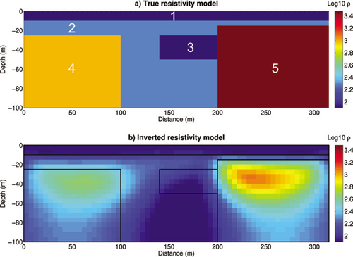
Synthetic fractured resistivity model representing sharp lateral contrasts of electrical resistivity between different rock formations that are more or less fractured. a) True resistivity model, b) inverted resistivity model. This synthetic model is based on a real case study (Robert et al. 2011 – site F5).
Seawater intrusion resistivity model
 , expressed as relative concentration, obtained from the density-dependent flow and transport simulations to the pore fluid electrical resistivity
  by means of the following relationship involving electrical conductivities
  and
and  of the freshwater and seawater, respectively:
 (3)
(3)In this study, we used representative values such as  and
and  (Nguyen et al. 2009).
 and the pore fluid resistivity
  as follows (Archie 1942):
 (4)
(4)The quantity  represents the so-called formation factor and reflects the choice of a homogeneous geological model for the seawater intrusion synthetic case study. The porosity,
  , was set to 0.35, the cementation exponent, m, was set to 1.5 and the tortuosity factor, a, was set to 1, which is valid for unconsolidated sediments (Schön 2004). For this numerical case, we assumed fully saturated conditions so that the saturation parameter,
  , is equal to 1. The resulting resistivity distribution is presented in Fig. 2(a).
For the ERT simulation, we used a finite element mesh composed of 25 × 6.1 m cells where 25 m is the unit electrode spacing used in the chosen configuration. We used a standard skip-1 dipole-dipole array (‘1’ denoting the number of electrodes that are skipped by each dipole) with 177 electrodes (for a total length of 4400 m) and  to calculate our data through forward modelling. Results of the inversion are presented in Fig. 2(b).
CONTAMINATED MODEL
The synthetic contaminated model was developed to appraise the ERT image quality of shallow and highly heterogeneous environments. The model was directly inspired by a real contaminated site located in the alluvial plain of the Meuse River near the city of Liege (Belgium).
Uncontaminated resistivity model
Previous geophysical studies conducted in this type of environment (Rentier 2002) allowed to estimate a magnitude order of electrical resistivity for each layer of the synthetic model. This latter is composed of four layers with different thicknesses and different electrical properties. The upper layer represents backfill deposits (thickness between 1–3 m) that have a high degree of heterogeneity and is composed of materials whose electrical resistivity ranges from 80–400  . The backfill layer overlays a more homogeneous fluvial silty-clay unit (average resistivity of 30
  ) with more resistive fine sand lenses for a total thickness between <1 and 4 m. Below these two units, we find alluvial sands and gravels (thickness between 2–6 m). The gravel layer has an average value of
  . Less resistive sandy lenses (
 ) are also present within this layer. The lower layer, the bedrock, is made of shale and sandstones and is set to a homogeneous resistivity value of
  . The resulting resistivity model is presented in Fig. 3(a).
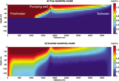
Synthetic saline intrusion resistivity model. a) True resistivity model, b) inverted resistivity model. We observe clearly the transition zone between freshwater ( ) and saltwater (
 ). A pumping well was simulated at a distance of 1800 m in order to induce saltwater upcoming in the aquifer.
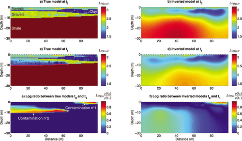
Synthetic contaminated resistivity model. a) and c) True resistivity models at time  and
and  , respectively, b) and d) associated inverted resistivity models. e) Logarithmic ratio between true resistivities at time
  and
and  , f) logarithmic ratio between inverted resistivities at time
  and
and  . e) and f) show the shape and magnitude of contaminated plumes.
Hydrogeological modelling
In order to simulate the presence of pollutants, two separate sources were introduced into the model: one in the first layer and the second in the third layer. The objective of this study is not to model the electrical response of a specific contaminant. Indeed, numerous factors depending mainly on the type and residence time of the contaminant in the underground may impact its electrical response. Biodegradation processes may, for example, play an important role as suggested in several studies (e.g., Sauck et al. 1998; Atekwana et al. 2000; Sauck 2000; Cassidy et al. 2001; Atekwana et al. 2002; Werkema et al. 2003; Atekwana et al. 2004,2004; Atekwana et al. 2005). These authors showed that when biodegradation occurs, areas contaminated by hydrocarbons, a common family of contaminants, tend to exhibit lower electrical resistivities than uncontaminated ones. Based on these findings, we chose to study the effect of a pollutant that increases the electrical conductivity of the pore water. For convenience, the pollutant considered is assimilated to saline water.
The transport of the contaminant is simulated by HGS. Two output times were extracted from the simulation,  corresponding to the uncontaminated situation and
  corresponding to the contaminated one.
Contaminated resistivity model
To build the resistivity model from the hydrogeological model, we partially followed the methodology outlined in Radulescu et al. (2007).
 (5)
(5)where  is the pore fluid resistivity,
  the relative concentration of the contaminant and
  and
and  , the electrical conductivities of uncontaminated water and the contaminant, respectively. In this model, we used
  and
and  .
.
 (6)
(6)where  is the electrical bulk resistivity and
  the formation resistivity factor (different for each layer). In our case,
  corresponds to the electrical bulk resistivity of the uncontaminated model and
  .
.
 , using the following relation:
 (7)
(7)The resistivity model impacted by the contaminations is presented in Fig. 3(c).
NUMERICAL BENCHMARK ON SYNTHETIC EXAMPLES: RESULTS AND DISCUSSION
The discussion presented in this section is organized following two main aspects. We first apply the edge detection approaches on the fractured and contaminated models. Secondly, we use other indicators to estimate the reliability of inverted parameters both quantitatively and qualitatively.
For all inverted models presented below, the data are fitted to their error level in order to reach a RMS of the chi-square variable of the error-weighted data misfit equal to 1.
Identification of the geometry of buried structures
For the first numerical benchmark, the detection of fractured zones is important as in reality they often represent zones where ground-water flow occurs. Detection of the shape of contaminant plumes is also important in reality in order to set up a monitoring network and/or to take remediation actions. In this scope, the second model is also particularly suited to the edge detection algorithm.
Fractured resistivity model
As shown in Fig. 1(a), the model is made of 5 different units with low- to high-resistivity contrasts. We want to determine which parts of the inverted model provide pertinent information on the geometry of the true model. First, we can study visually how the inversion process succeeds in reconstructing the 5 structures of the true model. Results of the inversion presented in Fig. 1(b) show that the 5 structures are identifiable even if a loss of geometry comes at depth (particularly visible for structures 3–5). However, this interpretation is biased by the fact that the true geometry is known and the same colour scale for both true and inverted models is used. Geometry identification would be more difficult without this a priori information. This highlights the need to resort to automatic edge detection in order to decrease the subjectivity associated to the user’s interpretation.
Automatic edge detection provides results that have to be interpreted cautiously. Detected edges can have different shapes in function of several parameters that have to be defined (type and size of noise reduction filter and threshold values applied on the gradient intensity).
We see in Fig. 4(a) that the watershed algorithm succeeds in retrieving the main structures. Contrarily to the visual interpretation, structures 4 and 5 are correctly delineated up to the base of the model. However, we observe that the algorithm tends to oversegment the image particularly when the size of the median filter (expressed in number of cells around the parameter of interest) is small. This is a well-known issue with this algorithm (Beucher 1994). To avoid this, more complex methods have been developed (e.g., Beucher 1994; Hui 2009) but their application is out of the scope of this work.
Figure 4(b,c) shows the edges detected with Canny’s algorithm. We observe that they vary with the standard deviation,  , of the Gaussian filter applied on the gradient image and with the thresholds applied on the intensity of the gradient image. Contrarily to the watershed results, there is no over-segmentation. The boundary between structures 1 and 2 is reasonably well retrieved for
  and small threshold limits:
  to 10−4 and
  to 10−3. The upper limit of structure 3 is also recovered using the same parameters but the localization error is larger and the algorithm is unable to detect its extent at depth. The edges of the main resistive structures (4 and 5) are not so well imaged, particularly at depth, using
  . However, when
  is increased, these latter structures are well detected even at depth with small localization errors but information on other edges is lost.
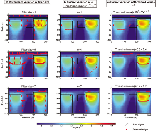
Automatic geometry detection applied on the fractured resistivity model using a) the watershed algorithm, b) and c) Canny’s algorithm. We see that detected edges depend on a) the size of the median filter, b) the standard deviation on the Gaussian filter and c) the thresholds applied on the gradient intensity. The watershed algorithm tends to over-segment the image though the main structures remain identifiable. Canny’s algorithm detects correctly the structures defined by the larger resistivity contrasts but seems to be less sensitive to smaller ones.
Contaminated resistivity model
We tested the algorithms on the contaminated resistivity model to check their ability to detect contaminant propagation between two resistivity images taken at different times (Fig. 3e,f).
Again, we observe different results in function of the parameters chosen for the algorithms (see Fig. 5). Edges detected by the watershed algorithm are too numerous for small filter sizes. For larger sizes, the number of edges decreases but the localization error tends to increase. This is particularly visible for the upper contaminant plume using a median filter size of 7. In this context, the watershed algorithm does not seem to be the most suited to delineate the extent of more complex geometries such as the ones of the contamination.
Canny’s algorithm provides results that are more easily inter-pretable because it avoids a too large over-segmentation (see Fig. 5b,c). We notice that the upper contaminant plume is well detected on the images with  . For larger
  , its lateral extent is underestimated and its extent at depth is overestimated. The upper boundary of the deeper contaminant plume is correctly detected on images with
  . However, the lower boundary cannot be recovered. This is not a problem due to the edge detection algorithms but to inversion limitations.
The automatic edge detection algorithms yield valuable information on the geometry of buried structures, information that is not always evident to find with only user’s interpretation. However, as described above, it remains difficult to detect automatically with certainty all edges on resistivity images without user’s intervention. This is why we recommend using these automatic approaches more as an aid rather than as infallible detection methods.
RELIABILITY OF INVERTED PARAMETERS AND ANALYSIS OF SPATIAL DISTRIBUTION
We now test the ability of the inversion process to recover the resistivity values of individual parameters using the different aforementioned appraisal indicators.
Seawater resistivity model
The seawater resistivity model (Fig. 2) is particularly suited to this analysis because the resistivity value of individual cells is directly related to the saltwater concentration by equations (3) and (4). We present in Fig. 6(a) the mean cumulative and individual absolute errors on recovered saltwater mass fraction ω in function of selected appraisal indicators and in Fig. 6(b) the spatial distribution of retrieved parameters for a threshold on the appraisal indicators corresponding to a mean cumulative error of 0.05 (see red lines in Fig. 6a). This value is chosen sufficiently small to recover the saltwater mass fraction with enough reliability and to avoid as much as possible the selection of parameters with too large errors.
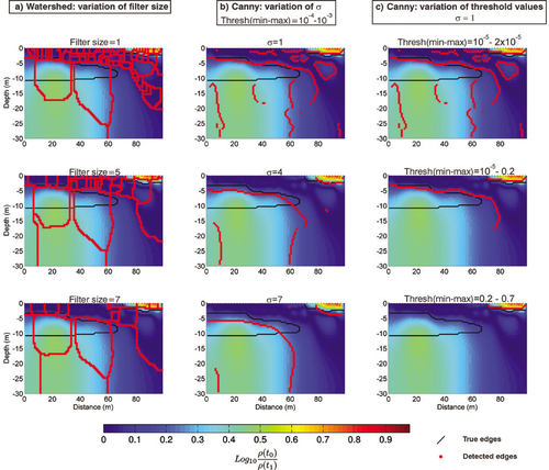
Automatic geometry detection applied on the contaminated resistivity model using a) the watershed algorithm, b) and c) Canny’s algorithm. We notice in this case that the geometries of contaminant plumes detected by Canny’s algorithm are closer to the true geometries than the ones detected by the Watershed algorithm.
 , as:
, as:
 (8)
(8)where  is the number of parameters characterized by an indicator value
  (for
(for  and
and  ) or
) or  (for
(for  and
and  ),
),  is the saline mass fraction derived from the inverted parameters that fulfil this criterion and
  the corresponding true mass fraction.
We first observe in Fig. 6(a) that the error distributions for the indicators  and
and  exhibit the same pattern with generally low errors for parameters with ‘ideal’ indicator values. The mean cumulative error curve shows a general growth trend as we move from ‘good’ to ‘bad’ indicator values quantified as recovered with a mean cumulative absolute error below and above 0.05, respectively. In this way, they seem to be particularly adapted for a quantitative appraisal as it is clearly possible to pick a value of the indicator and to estimate the error on the inverted parameters for a desired level of confidence. We note that for the chosen error threshold,
  is the indicator that selects more parameters, though results provided by
  and
and  are very similar.
 error distribution is quite different. We observe that for
  values close to zero (meaning that the inverted parameters depend very little on the reference model), the associated errors are not necessary small. This becomes particularly clear with the mean absolute error curve that does not show a general growth trend and where it is not possible to define a threshold on the indicator for the error level of 0.05. Therefore,
  does not seem to be as suited as the other indicators for a quantitative appraisal of parameters in this case.
In Fig. 7, we plotted the spatial distribution of parameters for the different appraisal indicators. For each indicator, we show four different captions corresponding to logarithmically equally spaced values ranging from the minimum to the maximum of the indicator, excluding these extrema in the representation.
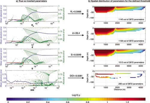
Absolute error on recovered saltwater mass fraction,  , in function of selected appraisal indicators. We notice that for a same mean absolute error on
  , we select more parameters with
  , though the diagonal of
  and
and  provide similar patterns. Moreover, the good values of these indicators are generally associated with small errors. This is not the case with
  that will not necessarily seek first the most reliable parameters.
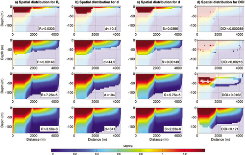
Spatial distribution of inverted parameters in function of different values of appraisal indicators. We generated six logarithmically equally spaced values from the minimum to maximum of the indicators, excluding these latters in the figure. We observe that  ,
,  and
and  exhibit the same pattern while
  shows more erratic distribution, at least for the first three threshold values.
The spatial distribution for  and
and  (see Fig. 7a–c) is coherent because they first select the parameters close to the surface where normally parameters are more reliable. The distribution of the parameters for these indicators is also gradual, meaning that for each bin, we retrieve more or less the same number of parameters.
Concerning the  (see Fig. 7d), the distribution is more erratic at least for the first three thresholds. Parameters whose
  values are ideal (meaning close to zero) are not necessary those close to the surface. Moreover, we notice that for the first three thresholds of
  , we do not recover lots of parameters (only 16.7% for
  < 0.0162), meaning that most of the information included in the
  is provided in a relatively short range compared to other indicators. For the fourth chosen threshold, all four indicators show a similar pattern of recovery.
Contaminated resistivity model
The magnitude of the observed resistivity changes is directly related to the magnitude of the contamination by equations (5)–(7). To quantify the degree of contamination with ERT images, it is thus necessary that the inverted parameters be as reliable as possible.
We apply the same approach as for the seawater intrusion but this time, we choose to work directly with the absolute resistivity changes between the  and
and  images (see Fig. 8).
We observe that for a same threshold on the mean absolute error, set to a value of  , indicators based on
  and
and  provide again the same pattern of recovery. According to our threshold criterion, it appears that the first contaminant plume is well-imaged as the upper boundary of the second contaminant plume. As expected and shown in the edge detection section (see Fig. 5), the lower boundary of the second plume is not properly imaged during the inversion.
The  pattern of recovery exhibits again a very different behaviour. For a same threshold on the mean absolute error,
  recovers only half of the parameters relative to
  or
or  , meaning again that small
  values are less associated to small absolute errors than these latter indicators.
Note about 
The results shown above tend to suggest that  is not the most suited tool to appraise quantitatively ERT images. However, when initially described in Oldenburg and Li (1999),
  was not presented as a quantitative tool but rather as a qualitative tool providing mainly information about the depth below which the parameters are no more constrained by the data. To check the information provided by
  about the depth of investigation, we present in Fig. 9 the maximum gradient line of
  (dashed red line) detected with Canny’s algorithm for the three numerical models. In order to compare it with another indicator, we also present the maximum gradient line of
  (dashed yellow line). The maximum variations of
  and
and  , located in the upper cells of the models, do not provide much information and are therefore not shown in Fig. 9.
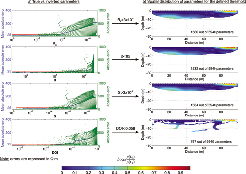
Absolute error on recovered resistivities in function of selected appraisal indicators. We notice that for a same mean absolute error, we select more parameters with the diagonal of  , though again
  and
and  provide a similar pattern.
  exhibits again a very different spatial distribution.
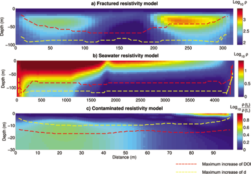
Maximum increase lines of  (dashed red) and
  (dashed yellow) for the three synthetic models providing mainly qualitative information about the assumed depth below which data no more constrained the model parameters. For a qualitative appraisal,
  seems to be the most suited tool.
We observe that for the fractured model (Fig. 9a), the boundary defined by  is located at the same depth, i.e., between –40 and –60 m, as the depth where the geometries of structures identified by the edge detection algorithms begin to diverge slightly from the true geometries (see Fig. 4). The maximum increase line of
  is located deeper and can hardly be interpreted as a sudden loss of information.
The limit defined by  for the seawater intrusion model (Fig. 9b) is located at a depth of around –80 m at the level of the transition zone between fresh- and seawater where the resistivity contrast should be higher. Visual validation of this limit can be made by looking at the area below, comprising a distance between 0–1000 m, where it is obvious that the inverted model parameters are not as well imaged as the upper parameters. The limit defined by
  exhibits the same shape but is shifted approximately 30 m downward compared to
  .
.
Concerning the contaminated model (Fig. 9c), we know that the base of the second contaminant plume has a maximum depth of approximately –10 m. This latter is not reproduced on the inverted model. The maximum increase lines of  and
and  , found between –10 and –15 m, are more or less consistent with observations.
These results tend to suggest that  is the most suited indicator for a qualitative appraisal of ERT images.
METHODOLOGY PROPOSED FOR A QUANTITATIVE APPRAISAL
We showed that it was possible to set a threshold on the indicators when the errors on the model parameters are known. However, it is difficult to find one general threshold of an indicator for all situations since many factors influence this value, e.g., number of data, data quality, type of electrode array or the complexity of the medium. In reality, it is also difficult to estimate the error of model parameters as the true resistivity distribution is generally unknown.
Therefore, in order to appraise quantitatively an ERT image using appraisal indicators, we propose an innovative methodology, illustrated in Fig. 10, which is based on the creation of synthetic models. It can be decomposed into several successive steps:
1. Acquisition and inversion of field electrical data → Real inverted model.
2. Creation of a synthetic resistivity model based on a combination of available information (e.g., borehole data) and the real inverted model → True synthetic model.
3. Forward modelling on the true synthetic model → Synthetic geophysical data.
4. Inversion of the synthetic geophysical data → Synthetic inverted model.
5. Comparison between the true and inverted synthetic models → Threshold on the resolution indicator.
6. Application of the threshold on the real inverted model → Truncated real inverted model.
7. Validation (and eventually correction) of the results by comparing the truncated real inverted model and available punctual information → Validated real inverted model.
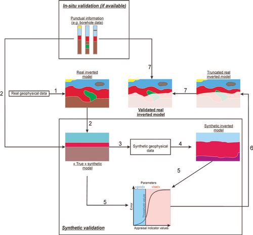
Multistep methodology proposed to assess the correctness of recovered parameters of an inversion. Step 1: inversion of real ERT data → Real inverted model. Step 2: creation of a synthetic resistivity model based on the real inverted model and a priori information → True synthetic model. Step 3: forward modelling on the synthetic resistivity model → Synthetic ERT data. Step 4: inversion of synthetic ERT data → Synthetic inverted model. Step 5: comparison between the true synthetic model and the synthetic inverted model in order to define a threshold value on the appraisal indicator in function of the level of confidence desired. Step 6: application of the threshold value on the real inverted model → Truncated real inverted model. Step 7: comparison between the truncated real inverted model and a priori information in order to validate the approach → Validated real inverted model.
FIELD EXAMPLES
Havelange site
This site is located in the city of Havelange (province of Namur, Belgium). Results of geophysical and hydrogeological studies carried out on this site were published in Robert et al. (2011, 2012). One of the objectives of the geophysical investigations was to provide the best location for the positioning of a ground-water monitoring well.
The geology encountered on the site is composed of a superficial loamy layer of approximately 5 m thickness. The underneath bedrock is composed of limestone with locally fractured zones. Figure 11(a) presents the inverted model obtained with a dipoledipole array ( ) with 122 electrodes spaced 5 m. Low resistivities found near the surface are related to the overburden and the weathered part of the bedrock. At depth, we find more resistive structures (up to 850 Ω.m) that are associated to unaltered bedrock. More conductive zones are present between 250–400 m and 450–500 m along the profile. A thinner and less visible conductive zone is also present between 100–160 m. These latter structures suggest local geological anomalies (fractures/karsts).
A drilling campaign was conducted according to geophysical results. A well was drilled in the anomaly located between 100–160 m (exact well location is 120 m) because fractured zones are assumed to be major groundwater flow pathways.
Geological information from the borehole showed that the well indeed crossed a lot of fractures and provided very high yields. The critical discharge was estimated to be more than 20 m3/h and hydraulic conductivity to be 10−4 m/s after the pumping tests (Robert et al. 2011).
In order to confirm the ability of the ERT image to provide information about the fracturing, we applied Canny’s algorithm without any noise reduction filter. Detected edges are presented in Fig. 11(b). We notice that the previously identified anomalies are well retrieved. Unaltered bedrock zones are particularly visible. The more conductive zone where the well was drilled seems to be, as expected, a fractured zone separating two unaltered limestone units. The limit defined by the maximum increase of  is located at an elevation of approximately 210 m at the place where the well was implemented (see Fig. 11b). This suggests that the results provided by the edge detection algorithm above this limit can be interpreted since they relate to areas of the model still constrained by the surface data. Given the objective of the study, a further quantitative appraisal is not necessary in this case.
Maldegem site
This site is located in the city of Maldegem (province of East Flanders, Belgium) and presents contamination in chlorinated solvents (common DNAPLs). This is historical pollution (pollution took place from 1951–1981). The contamination is linked to the former activities of the site dedicated to dry cleaning.
From the few samplings carried out during the characterization study, it appears that the initial contaminant, Tetrachloroethylene (PCE), has undergone a natural process of anaerobic degradation, called halorespiration (Alvarez and Illman 2006), leading to the detection of degraded compounds such as Trichloroethylene (TCE), Dichloroethylene (DCE) and Vinyl chloride (VC) that are also hazardous compounds for the environment. However, the characterization study did not allow to clearly detect the location of the source of the contamination or its extent (see Fig. 12).
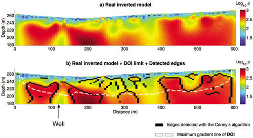
Qualitative appraisal on the Havelange site with the edges detected by Canny’s algorithm (black cells) and the maximum gradient line of  (dashed white line).
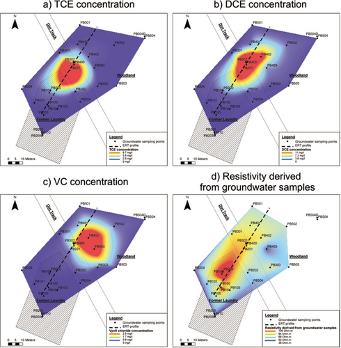
Map of the contaminated site of Maldegem. a) TCE concentration, b) DCE concentration, c) VC concentration and d) bulk electrical resistivities derived from groundwater electrical conductivities. Groundwater flows are directed from south-west to north-east. The initial contamination in PCE is suspected to have taken place near boreholes PB102 and PB200.
From a geological point of view, the site can be decomposed into an upper layer of soil made of quaternary sand overlying a clay layer found at –11 m according to available borehole data. The clay layer can be considered as a hydraulic barrier preventing the downward migration of contaminants. Available piezometric data indicate a groundwater flow direction from southwest to north-east. The groundwater table is found at a depth of –1.8 m in the southern part of the site and at a depth of –3.7 m in its northern part.
Inversion of field data
The goals of the electrical investigations after the characterization study were first to detect the source of the contamination, then to delineate its extent and finally to assess its magnitude. The ERT profile was oriented in order to pass over the main contaminated areas as revealed by chemical analysis (see Fig. 12).
Figure 13(a) presents the inverted model obtained with a Wenner-Schlumberger array ( ) with 72 electrodes spaced 1 m. Several electrical structures can be observed. Very resistive areas found near the surface from the middle of the profile to the north-east correspond to the unsaturated zone combined with an effect of tree roots as this part of the profile is located in woodland. We also observe a very conductive zone
  ) found at a depth that is probably related to the clay layer. The most interesting electrical structure is visible at a distance between 6–32 m and at a depth between –2 and –9 m. It shows some resistivity contrast with the rest of the area (with resistivities ranging from
  ). At first sight, it is located upstream of the main detected concentrations of TCE and DCE (see Fig. 12). By analysing in detail the chemical data, we see that the centre of the anomaly is located near the boreholes (PB102 and PB200) where PCE has been detected in groundwater at –5 m depth. The ERT results seem to suggest that the location of the initial source of pollution is located close to this main anomaly, in a zone where there are relatively few borehole data.
Another anomaly, characterized by a lower resistivity contrast, is also visible in the area where the highest concentrations of TCE and DCE were detected. The lower resistivity contrast in this zone could be explained by the effect of biodegradation that would tend to decrease the fluid resistivity.
The results of the ERT profile are consistent with the measurements of electrical conductivity on water samples. These latter are converted to resistivities using Archie’s formula assuming a formation factor of 4. A resistivity map based on water samples is illustrated in Fig. 12d. It clearly shows a more resistive zone near the main anomaly, which demonstrates that the latter cannot be related to a different geological material but rather to a fluid with different properties that are more than likely impacted by the contaminants.
We applied Canny’s algorithm without any noise filter on the image. Edges detected are presented in Fig. 13b (black cells). The algorithm provides edges in the upper part of the model that are related to the piezometric level. Thus, it offers indications on the transition between unsaturated and saturated sands. Below this first structure, we observe another one that has the shape of a plume that plunges towards the northeast. It coincides with the previously described resistive anomaly and is associated to the contaminant plume. The continuity and extent of the detected structure are coherent with our hypothesis of a contaminant plume and with the chemical analysis.
Synthetic resistivity model
In order to assess the reliability of real inverted parameters, we developed a synthetic resistivity model (see Fig. 13c) using available borehole data to image the clay layer, piezometric data to image the groundwater table and finally the shape of the assumed contaminant plume to image the contamination.
After inversion, the plume anomaly is partially recovered in the southern part of the image even if its vertical extent is overestimated due to the smoothing. The part of the plume that plunges towards the north is clearly less visible.
In order to define a threshold on the appraisal indicator (we chose the diagonal elements of  ), we compared the true and inverted synthetic models. We observe in Fig. 13(e) that the relative error on the inverted parameters increases more rapidly from a value of
  allowing the definition of a threshold. By using this threshold, the mean relative error on the remaining parameters is approximately 25%. This value seems sufficiently small though its choice may be subject to discussion.
Application of the threshold value on the field ERT image is illustrated in Fig. 13(f). The plume anomaly appears to be well-imaged (according to the chosen error criterion) until a depth of –5 m. The parameters corresponding to the northern and deeper part of the plume are not recovered because they are associated to too large errors. In summary, for a quantitative use of inverted parameters with an expected mean relative error of 25% (for example to develop a relation between resistivities and contaminant concentrations), it is advised to work with the selected parameters.
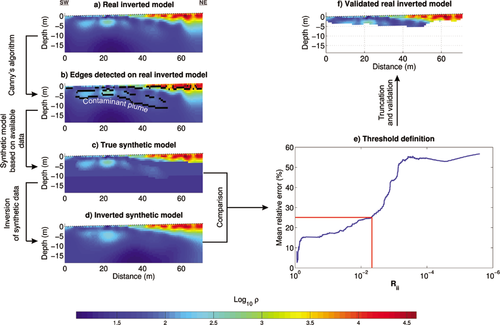
Quantitative methodology applied on the Maldegem site. a) Real inverted model corresponding to field data, b) edges detected on the real inverted model with Canny’s algorithm, c) synthetic resistivity model built using available information coming from field observations and from structures detected with the edge detection algorithm, d) inverted synthetic model, e) comparison between the true and inverted synthetic models in function of the diagonal elements of  and definition of a threshold value and f) application of the threshold value on the real inverted model.
CONCLUSIONS
From our study, whose main achievements are summarized in Table 1, indicators based on  and
and  appear to be more suited than
  for a quantitative appraisal because they allow selecting parameters that present generally low errors and that are homogeneously distributed. The diagonal elements of
  and
and  provide almost the same results. For a qualitative appraisal, meaning being able to define a ‘limit’ on the model where the influence of data on the solution becomes insignificant (which is somehow hard to define),
  seems to be the best tool. Rather than choosing the limit on
  using a predefined value (usually 0.1 or 0.2), we suggest to use the maximum gradient line of
  . For automatic edge detection, the Watershed algorithm tends to over-segment the image providing more structures than there are actually. Used alone, it can hardly help the user in the interpretation of buried structures. Results provided by Canny’s algorithm are easier to interpret. The algorithm avoids the over-segmentation but requires providing two threshold values on the gradient intensity in order to define the actual crest lines. This can lead to missing some structures if these values are not well-defined. Further adaptations of the algorithm are thus needed to make it fully usable for ERT imaging.
When no ground truth is available to define a threshold on the appraisal indicators, we propose a methodology based on the results acquired with numerical benchmarks to appraise both qualitatively and quantitatively an inverted resistivity model. Both methodologies were applied on field ERT images with valuable results.
This study has also highlighted the difficulty to define threshold values on the appraisal indicators. The discrepancy between the true and inverted models in function of the indicator does not always show a significant increase. We also noticed that the type of discrepancy measurement is very important for the appraisal result. For environments exhibiting very low resistivities, the relative error between the true and inverted parameters can be drastically high, while in the same time the absolute error is very low. The opposite reasoning can be made for very resistive environments. The type of discrepancy measurement will finally depend on the objectives to be achieved. The acceptable error level can also be difficult to assess as was shown in all tested cases. This may introduce some subjectivity in the threshold definition. To overcome these problems, efforts must be made to develop new indicators more suited for a quantitative use such as the more comprehensive analyses proposed by Singha et al. (2007).
ACKNOWLEDGEMENTS
We would like to thank the associate editor and reviewer for their pertinent comments and suggestions, which have helped to improve significantly this manuscript. We also thank FRIA (FNRS-Belgium) who financed this study.
| Main achievements of the numerical benchmark + Pros and cons of the proposed appraisal methodologies. | ||
|---|---|---|
- Edge detection algorithms useful to help the practitioner to interpret buried structures but require some expertise -
- |
||
| Qualitative approach:
|
Quantitative approach:
|
|
| + | - No synthetic models - No prior knowledge of the subsurface - Help the practitioner to detect buried structures - Provide a “limit” where the reference model takes precedence over the data |
- Innovative and easy to implement - Estimation of the error on inverted parameters - Provide an appraisal on the whole ERT image - No ‘ground truth’ needed |
| − | - Difficulty to define the damping factor of the reference model for - No estimation of the error on inverted parameters |
- Synthetic models with prior knowledge of the subsurface (ideally) - Difficulty to define the threshold values on the appraisal indicator |


 and
and  provide similar results and allow selecting homogeneously distributed parameters with low errors contrarily to
 and
and  more suited for a quantitative appraisal
 more suited for a qualitative appraisal
 limit defined by the maximum gradient line more relevant than by a predefined isocontour
 and edge detection algorithms
 or
or  and synthetic resistivity models
 and the thresholds on the gradient intensity for the edge detection