Use of a sub-array statistical approach for the detection of a buried object
ABSTRACT
A hybrid electromagnetic-statistic approach for the detection and localization of a perfectly-conducting circular cylinder, buried in a lossless half-space, is presented. We use the results of a cylindrical wave approach forward solver as input data for our detection procedure. We use a sub-array processing structure and apply several algorithms for the direction of arrival estimation. By triangulating the found directions of arrival, a set of crossings, condensed around the object locations, is obtained. To process the crossing pattern, we developed a statistical model for the crossings distribution and employed hypothesis testing procedures to identify a collection of small windows containing the target. By defining a suitable threshold from a desired false alarm rate and dividing the region in small windows it is possible to ascribe each window to the ground or to the object. Numerical results are presented for a cylinder in a vacuum and in a dielectric half-space, both in a central and in a peripheral position with respect to the array centre. Different values of the cylinder radius and of the distance from the array are considered.
INTRODUCTION
Non-invasive identification of buried objects in the near-field of a receiver array is a subject of great interest, due to its application to the remote sensing of the earth’s subsurface (Daniels 2004; Armand and Polyakov 2005), environment reclamation (such as the detection of landmines; Geneva International Centre for Humanitarian Demining 2006), civil engineering (like the localization of pipes and conduits; Xiaojian, Haizhong and Huiliang 1997), archaeological investigation and more (Pirri, Lombardo and Bucciarelli 2000).
In general, the reconstruction of a scenario starting from the scattered electromagnetic field is a heavy problem and its solution has involved many authors with different approaches. Because of the intrinsic non-linearity of the inversion, some approximations (Born, Rytov, Kirchhoff, etc.) are considered in many works (e.g., Devaney 1981; Zapalowski, Fiddy and Leeman 1984; Mayer 2002; Soldovieri and Solimene 2007); moreover, numerical or iterative methods to solve the non-linear problem (e.g., Bojarski 1982; Chiu and Kiang 1992) have been proposed.
Some techniques, very popular in a smart antennas context, like the direction of arrival ones, are still adopted in radar applications to localize signal sources and targets (Shan, Wax and Kailath 1985; Chandran 2005; Balanis and Ioannides 2007; Dmochowski, Benesty and Affes 2007; Grice et al. 2007). The synergy between signal processing and electromagnetic areas was introduced several years ago in many works, as in Bruckstein and Kailath (1987) and Şahin and Miller (2001).
In this paper, we present a statistical approach to process the data calculated by a forward scattering solver, in order to find an estimation for the position of an object using a sub-array processing technique (Bouvet and Bienvenu 1991; Krim and Viberg 1996) similar to the one presented in Şahin and Miller (2001). Moreover, sub-array processing techniques have been considered in order to achieve localization also for objects in the proximity of the array (Schmidt 1986).
We apply the approach to many directions of arrival estimation methods and compare their performances in several scenarios. The forward scattering problem is solved with the cylindrical-wave approach (Di Vico et al. 2005).
The direction of the arrival approach assumes that the sources are in the far-field region of a receiving array, so that the received wavefront could be considered as planar. By dividing the whole array in a certain number of sub-arrays and finding the dominant direction of arrival for each one, it is possible to localize objects in the far-field of the sub-array even if they are in the near-field of the array.
In the first step of the detection procedure, we apply several directions of arrival techniques to obtain a set of angles for each sub-array. By triangulating these directions we obtain a collection of crossings crowding in close proximity of the object.
In a second stage, the crossings are modelled as Poisson distributed points, with a large rate parameter around the target and a low rate parameter in the ground region. In this way we can separate two types of regions: one, corresponding to the large rate distribution, is represented by a large number of crossings very close to each other, while the second region is a cloud of less dense crossings that are considered as the background. A testing procedure is employed to determine a set of window regions corresponding to the target area and finally the cylinder coordinates are extracted. The procedure is schematized in Fig. 1.
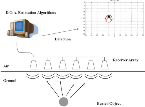
Scheme of the scattering problem and the detection procedure ‘Signals and noise model’.
We apply the procedure in two different situations. First, we simulate several settings in a vacuum, in order to verify the intrinsic capabilities of the direction of arrival methods and the detection procedure in terms of object dimension and its distance from the array. We then simulate some cases in half-space geometry, with the array sensors adhering to the medium in which the cylinder is buried. Our purpose is to verify the performances of the direction of arrival algorithms in a dielectric homogeneous half-space different from air.
The paper is organized as follows. In the section ‘Signals and noise model’, a model for the received signals and noise is presented and the steering vector representation is introduced. In the section ‘Pseudospectrum and direction of arrival estimation’, a brief description of several directions of arrival methods is provided. The section ‘Sub-array localization procedure’ is devoted to the sub-array processing statistical procedure, while in the section ‘Numerical results’ the numerical results are presented and discussed. Finally, conclusions are drawn.
SIGNALS AND NOISE MODEL
We consider an array of  identical sensors uniformly spaced along a line, with period
  , as depicted in Fig. 2. It is commonly referred to as a uniform linear array.
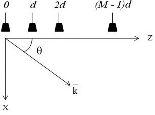
Uniform linear array scenario.
 indicate the direction of arrival of the signal coming toward the array at the
  -th receiver
  . Then, under the plane-wave hypothesis, we find that the output of the generic sensor
  is
is
 (1)
(1) and
and  are the angular response of the
  -th sensor (supposed to be the same for all the array elements) and the incoming signal, respectively;
  denotes the sensor position. Since
  and considering isotropic sensors, the steering vector
  is defined as:
 (2)
(2)In equation (2),  is the wavenumber associated to the plane wave propagating through the medium in which the object is buried. If this medium is different from the one in which the array is placed, the data obtained by solving the forward-scattering problem with the cylindrical wave approach take into account the refraction by the planar interface, while the inversion procedure neglects it. However, when the array is very close to the interface (as happens in several ground-penetrating radar (GPR) applications), the numerical error that affects the direction of arrival estimation assuming a homogenous medium is very small.
The  is a Vandermonde-like vector; thus a matrix of steering vectors
  can be built, with
  independent columns (Van Trees 2002). In the uniform linear array case,
  is uniquely defined if and only if the condition
  is fulfilled, which is always satisfied if the period
  is less or equal to half a wavelength. Also to avoid aliasing in space it must be
  (Şahin and Miller 2001).
 narrowband signals coming from different directions is sketched, with
  . Each received signal
  includes additive, zero mean, Gaussian noise. Time is represented by the
  -th time sample (
 where
where  is the total number of time samples); thus the array output
  can be given as (Gross 2005):
 (3)
(3) (4)
(4)being  the array weights;
  and
and  are the incident signals vector and the noise vectors, respectively, at the time instant
  .
.
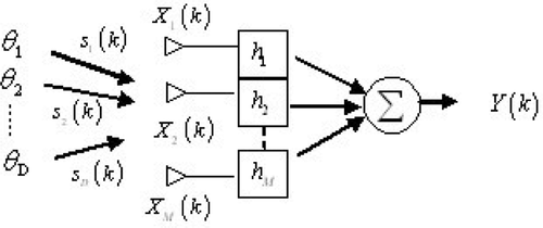
Receiving array and relevant signals.
 Hermitian array correlation matrix
  can be defined as:
 (5)
(5)where  is the source correlation matrix, while
  is the
  noise correlation matrix;
  symbolizes the hermitian transposition.
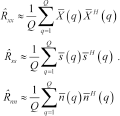 (6)
(6)PSEUDOSPECTRUM AND DIRECTION OF ARRIVAL ESTIMATION
 , is given by the square magnitude of the array output, which is
 (7)
(7) can be modelled as zero-mean stationary processes, for a given weight vector
  , the mean output power of the array system is obtained by calculating the conditional expectation over
 (8)
(8)It is clear that the pseudospectrum function is strongly depending (through  ) on
) on  and the particular choice of the vector
  differentiates the direction of arrival estimation algorithms. We analysed and implemented several methods: Bartlett and Capon beamforming, maximum entropy, linear prediction, Pisarenko harmonic decomposition, minimum norm and multiple signals classification.
The non-parametric methods of spectral estimation (Bartlett and Capon algorithms) do not make any assumption on the covariance structure of the data. They suppose that the functional form of the steering vector  is known, characterizing the array as a spatial sampling device. The parametric, or modelbased, methods (linear prediction, maximum entropy, minimum norm, Pisarenko harmonic decomposition, multiple signals classification), instead, assume that the signal satisfies a generating model with known functional form and then proceed by estimating the parameters in the chosen model.
Some parametric algorithms considered (linear prediction, Pisarenko harmonic decomposition, maximum entropy) are based on the autoregressive moving average models of the signals (Stoica and Moses 2005). The other algorithms are eigenvalue decomposition techniques (minimum norm and multiple signals classification) (Godara 1997).
 (9)
(9) represents uncorrelated monochromatic signals and there is no system noise, the Bartlett estimation is equivalent to the square magnitude of a spatial finite Fourier transform of all the arriving signals.
 (10)
(10) (11)
(11)The Capon method has a better resolution than the Bartlett direction of the arrival estimate. But, in the cases when the sources are correlated, the Capon resolution may become worse. The main advantage of these two estimation methods is that they are non-parametric solutions; therefore a priori information of the statistical properties of the signals is not needed.
 (12)
(12)where  is the Cartesian basis vector that is the
  -th column of the
  identity matrix. The particular choice of
  has a big influence on the prediction (Johnson 1982). This method is an autoregressive technique and the pseudospectrum peaks are proportional to the square of the signals power.
 :
:
 (13)
(13)where  is the
  -th column of the inverse array correlation matrix
  .
.
 can be used to minimize the mean-squared error. The corresponding pseudospectrum is given by
 (15)
(15)where  is the eigenvector associated with the smallest eigenvalue
  .
.
 (16)
(16)where  is the subspace of the M–D noise eigenvectors. It can be noted that this method combines all noise eigenvectors whereas the Pisarenko harmonic decomposition only uses the first noise eigenvector (Gross 2005).
The multiple signals classification technique was first introduced by Schmidt (1986). It is a high resolution eigenstructure method able to estimate the number of signals, the angle of arrival and the strength of the waveform, under the assumption that the noise is uncorrelated. The multiple signals classification algorithm generates two subspaces:  (noise) and
  (signal), from the eigenvectors associated with the eigenvalues of the array correlation matrix
  .
.
In particular, since the noise is uncorrelated, the smallest M–D eigenvalues of  are all equal among them and to the noise variance
  such as
  . The remaining D eigenvalues are greater, so
  where
where  . is the
  -th positive eigenvalue of the hermitian
  matrix
  .
.
 are obtained by M–D eigenvectors associated with the smallest M–D eigenvalues of
  and are orthogonal to the array steering vectors at the angles of arrival
  . Because of this condition, the Euclidean distance
  is equal to zero for each direction of arrival. The multiple signals classification pseudospectrum is finally given as
 (17)
(17)SUB-ARRAY LOCALIZATION PROCEDURE
The direction of the arrival approach assumes that the sources are in the far-field region of a receiving array, so that the received wave-front could be considered as planar. By dividing the whole array in a certain number of sub-arrays and finding the dominant direction of arrival for each one, it is possible to localize objects in the far-field of the sub-array even if they are in the near-field of the array. Therefore if  represents the size of the sub-array, the minimum distance attended for a successful object localization is
  .
.
After estimating the directions of arrival, we proceed by triangulating them, obtaining a crossing pattern, as the one reported in the upper side of Fig. 4. Two regions can be distinguished, the first one including a big number of crosses that most probably locates the target and a background region in which the amount of crosses is quite small and spread. The two classes of crossings are modelled using a pair of spatial Poisson distributions (Hoaglin 1980; Şahin and Miller 2001): the rate parameter of the background is considerably smaller than the one of the target.

A typical pattern resulting from directions of arrival triangulation.
For a given crossing pattern, we divide the region of interest into  uniform nonoverlapping windows of fixed size and count the number of crossings
  . The windows must be nonoverlapping to guarantee the independence of the random variable
  , which is the number of crossings in each window. The window dimensions affect the performances of the procedure and they must be optimized taking into account the size of the object to detect.
We suppose that  is Poisson distributed and check this assumption by using the graphical technique presented in Hoaglin (1980). It suggests to plot, in an iterative way, the quantity
  versus the count of crossings
  , where
  , is the number of occurrences of finding
  crossings in a window. If the plotted trend forms a straight line, with a slope approximating ln
  , it properly approximates a Poisson distribution of rate parameter
  .
.
A typical plot thus obtained is reported in Fig. 5. It is possible to interpolate the circles by tracing two different lines: one of them, with a positive slope, corresponds to a large value of  (greater than
  ) while the second one, with a negative slope matches the circles relative to smaller values of the crossing count
  (between 0 and
  ).
).
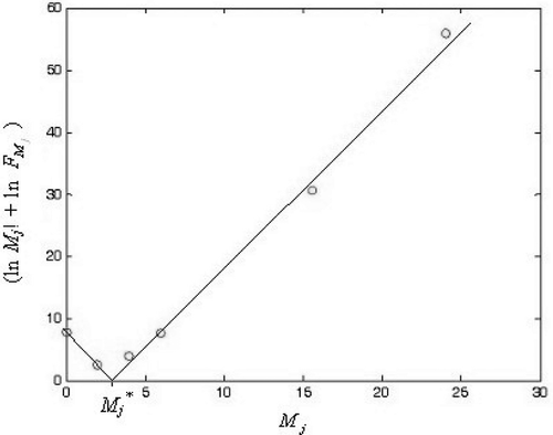
A typical plot of the quantity in  (circles), as a function of
  .
.
 (18)
(18) (19)
(19)where the quantities having subscript  and
and  are relevant to background and target, respectively, moreover
  and
and  represent the total amount of background and target windows, respectively.
 crossings) to belong to the background is:
 (20)
(20) (21)
(21) , with
  , where
  , is the number of overlapping windows in the region of interest. The hypothesis test is formally a binary one:
 is Poisson distributed with a small rate parameter
  ;
; is Poisson distributed with a large rate parameter
  .
.
 (22)
(22) can be determined from the desired false-alarm rate expressed as
 (23)
(23)We finally obtain an estimated crossing pattern like the one shown in Fig. 6.
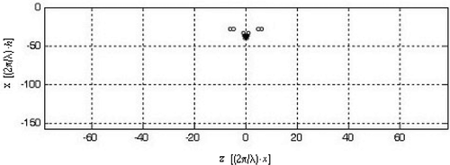
Refined crossing pattern of Fig. 4.
NUMERICAL RESULTS
A uniform linear array of 51 equally spaced elements is considered, with period  . A three-element sub-array partition is applied (the total number of sub-arrays is therefore 17). A perfectly conducting circular cylinder characterized by a radius
  , which has its centre located at a distance
  from the array axis. For this configuration, the cylinder is in the far zone of the sub-array if its burial depth is at least
  . The incident wave is TM polarized (electric field parallel to the cylinder axis). The noise variance is
  the false-alarm probability is 106.
 and
and  and using in the sub-array processing procedure square windows with side-length
  , also for the test windows. Objects and depths, both small and comparable to the operating wavelength, are considered. Moreover, a central and a peripheral position of the target are treated, with respect to the array geometry. We define the localization error as
 (24)
(24)where  and
and  are the real and estimated cylinder axis coordinates, respectively. The quantity
  is the ratio between the Euclidean distance of the estimated centre from the real one and the actual cylinder radius. When
  , the estimated centre is collocated in a point inside the cylinder transverse section, otherwise, if
  , the estimation of the centre falls outside the object. As a reference threshold, we assume that a target can be considered correctly localized if the error is less than 1. In Tables 2–5, some results are presented, with
  and
and  assuming the values here listed (the symbols a1–a5 and A–E will be used for reference in the following):
| a1 | a2 | a3 | a4 | a5 | |
Radius  |
 |
 |
 |
 |
 |
| A | B | C | D | E | |
burial depth  |
 |
 |
 |
 |
 |
 |
A | B | C | D | E | |
|---|---|---|---|---|---|---|
| Bartlett/Multiple signals classification | a1 | 6.236 | 6.060 | 5.824 | 4.930 | 5.597 |
| a2 | 2.224 | 2.120 | 1.512 | 1.525 | 1.537 | |
| a3 | 0.569 | 0.571 | 0.451 | 0.207 | 0.206 | |
| a4 | 0.271 | 0.079 | 0.078 | 0.015 | 0.145 | |
| a5 | 0.028 | 0.120 | 0.207 | 0.159 | 0.145 | |
| Capon | a1 | 6.623 | 6.568 | 6.917 | 6.308 | 5.880 |
| a2 | 2.246 | 1.847 | 2.276 | 1.596 | 1.726 | |
| a3 | 0.731 | 0.704 | 0.451 | 0.318 | 0.223 | |
| a4 | 0.249 | 0.117 | 0.204 | 0.100 | 0.201 | |
| a5 | 0.060 | 0.112 | 0.167 | 0.170 | 0.201 | |
| Linear prediction | a1 | 7.925 | 6.847 | 6.588 | 5.830 | 6.314 |
| a2 | 2.640 | 2.473 | 1.976 | 1.516 | 1.734 | |
| a3 | 0.759 | 0.646 | 0.591 | 0.428 | 0.224 | |
| a4 | 0.266 | 0.208 | 0.129 | 0.685 | 0.099 | |
| a5 | 0.220 | 0.299 | 0.312 | 0.174 | 0.005 | |
| Maximum entropy | a1 | 9.552 | 9.029 | 7.629 | 6.391 | 5.894 |
| a2 | 2.249 | 1.521 | 1.697 | 1.150 | 2.271 | |
| a3 | 0.577 | 0.578 | 0.550 | 0.608 | 0.365 | |
| a4 | 0.294 | 0.040 | 0.182 | 0.080 | 0.075 | |
| a5 | 0.211 | 0.277 | 0.288 | 0.301 | 0.397 | |
| Minimum norm | a1 | 60.034 | 5.945 | 50508 | 5.306 | 4.647 |
| a2 | 2.182 | 2.025 | 1.852 | 1.527 | 1.431 | |
| a3 | 0.617 | 0.600 | 0.417 | 0.4069 | 0.270 | |
| a4 | 0.216 | 0.132 | 0.115 | 0.098 | 0.149 | |
| a5 | 0.125 | 0.115 | 0.199 | 0.222 | 0.232 | |
| Pisarenko harmonic decomposition | a1 | 6.965 | 5.985 | 5.967 | 4.478 | 5.128 |
| a2 | 2.037 | 2.009 | 1.771 | 1.545 | 1.285 | |
| a3 | 1.068 | 0.654 | 0.514 | 0.276 | 0.206 | |
| a4 | 0.314 | 0.332 | 0.094 | 0.156 | 0.074 | |
| a5 | 0.177 | 0.057 | 0.186 | 0.131 | 0.113 |
 , central position. Same geometrical parameters as Table 2
 |
A | B | C | D | E | |
|---|---|---|---|---|---|---|
| Bartlett | a1 | 4.482 | 3.349 | 4.819 | 3.189 | 3.725 |
| a2 | 1.517 | 1.584 | 2.063 | 0.980 | 1.801 | |
| a3 | 0.732 | 0.670 | 0.331 | 0.249 | 0.191 | |
| a4 | 0.114 | 0.153 | 0.167 | 0.196 | 0.114 | |
| a5 | 0.590 | 0.447 | 0.063 | 0.057 | 0.273 | |
| Capon | a1 | 4.356 | 10.463 | 4.898 | 9.834 | 7.822 |
| a2 | 1.541 | 4.226 | 2.359 | 1.555 | 1.294 | |
| a3 | 1.203 | 0.393 | 0.867 | 0.544 | 0.483 | |
| a4 | 1.044 | 0.244 | 0.156 | 0.099 | 0.223 | |
| a5 | 0.209 | 0.041 | 0.432 | 0.309 | 0.166 | |
| Linear prediction | a1 | 4.062 | 3.535 | 7.644 | 5.241 | 4.342 |
| a2 | 5.365 | 2.108 | 1.253 | 2.806 | 0.991 | |
| a3 | 1.820 | 0.360 | 0.365 | 0.348 | 0.813 | |
| a4 | 0.271 | 0.570 | 0.164 | 0.260 | 0.236 | |
| a5 | 0.091 | 0.163 | 0.055 | 0.128 | 0.156 | |
| Maximum entropy | a1 | 13.275 | 2.880 | 3.767 | 8.505 | 14.780 |
| a2 | 1.557 | 3.570 | 1.503 | 1.235 | 0.878 | |
| a3 | 0.962 | 0.557 | 0.547 | 0.307 | 0.604 | |
| a4 | 0.060 | 0.303 | 0.277 | 0.039 | 0.201 | |
| a5 | 1.787 | 1.101 | 0.105 | 0.066 | 0.226 | |
| Minimum norm | a1 | 6.514 | 4.482 | 7.715 | 4.861 | 3.577 |
| a2 | 1.206 | 3.856 | 1.471 | 1.031 | 1.762 | |
| a3 | 0.701 | 0.372 | 0.358 | 0.400 | 0.277 | |
| a4 | 0.579 | 0.154 | 0.322 | 0.207 | 0.364 | |
| a5 | 0.050 | 0.198 | 0.132 | 0.042 | 0.121 | |
| Pisarenko harmonic decomposition | a1 | 14.059 | 6.375 | 6.029 | 3.723 | 4.843 |
| a2 | 3.722 | 1.593 | 0.877 | 1.691 | 1.130 | |
| a3 | 0.7163 | 0.738 | 0.766 | 0.304 | 0.406 | |
| a4 | 0.6743 | 0.276 | 0.920 | 0.204 | 0.080 | |
| a5 | 0.238 | 0.179 | 0.250 | 0.465 | 0.138 | |
| Multiple signals classification | a1 | 4.024 | 3.349 | 4.819 | 3.189 | 3.725 |
| a2 | 1.210 | 1.584 | 2.063 | 0.980 | 0.967 | |
| a3 | 0.670 | 0.828 | 0.350 | 0.248 | 0.191 | |
| a4 | 0.114 | 0.153 | 0.167 | 0.196 | 0.114 | |
| a5 | 0.651 | 0.371 | 0.063 | 0.013 | 0.273 |
 , central position
 |
A | B | C | D | E | |
|---|---|---|---|---|---|---|
| Bartlett/Multiple signals classification | a1 | 4.386 | 4.605 | 4.296 | 3.618 | 3.143 |
| a2 | 1.746 | 1.456 | 1.110 | 1.338 | 0.984 | |
| a3 | 0.640 | 0.461 | 0.557 | 0.365 | 0.408 | |
| a4 | 0.343 | 0.159 | 0.148 | 0.190 | 0.245 | |
| a5 | 0.105 | 0.106 | 0.113 | 0.073 | 0.094 | |
| Capon | a1 | 5.719 | 3.913 | 3.022 | 4.473 | 4.076 |
| a2 | 1.602 | 1.304 | 0.765 | 0.903 | 1.014 | |
| a3 | 0.486 | 0.563 | 0.522 | 0.556 | 0.445 | |
| a4 | 0.576 | 0.197 | 0.115 | 0.228 | 0.214 | |
| a5 | 0.156 | 0.116 | 0.124 | 0.068 | 0.125 | |
| Linear prediction | a1 | 3.851 | 3.196 | 3.724 | 3.714 | 3.058 |
| a2 | 1.523 | 2.837 | 0.942 | 1.305 | 1.197 | |
| a3 | 0.580 | 0.407 | 0.679 | 0.625 | 0.554 | |
| a4 | 0.358 | 0.224 | 0.217 | 0.181 | 0.282 | |
| a5 | 0.083 | 0.153 | 0.087 | 0.112 | 0.223 | |
| Maximum entropy | a1 | 5.309 | 30613 | 3.484 | 4.156 | 3.633 |
| a2 | 1.024 | 1.004 | 1.020 | 1.395 | 1.126 | |
| a3 | 0.595 | 0.438 | 0.849 | 0.464 | 0.318 | |
| a4 | 0.329 | 0.138 | 0.139 | 0.213 | 0.234 | |
| a5 | 0.133 | 0.148 | 0.132 | 0.162 | 0.183 | |
| Minimum norm | a1 | 4.054 | 4.517 | 4.200 | 3.652 | 3.089 |
| a2 | 1.702 | 1.444 | 1.073 | 1.395 | 1.069 | |
| a3 | 0.678 | 0.432 | 0.551 | 0.361 | 0.416 | |
| a4 | 0.326 | 0.191 | 0.154 | 0.201 | 0.218 | |
| a5 | 0.116 | 0.116 | 0.121 | 0.087 | 0.120 | |
| Pisarenko harmonic decomposition | a1 | 4.851 | 5.872 | 4.379 | 3.930 | 3.395 |
| a2 | 1.420 | 1.433 | 1.224 | 1.295 | 1.488 | |
| a3 | 0.376 | 0.518 | 0.626 | 0.297 | 0.550 | |
| a4 | 0.178 | 0.243 | 0.124 | 0.232 | 0.305 | |
| a5 | 0.554 | 0.087 | 0.130 | 0.124 | 0.253 |

 |
A | E | A | E | |
|---|---|---|---|---|---|
 |
 |
 |
 |
||
| Bartlett | a1 | 12.305 | 12.932 | 4.451 | 5.596 |
| a2 | 4.880 | 4.169 | 1.466 | 2.240 | |
| a3 | 1.931 | 1.211 | 0.519 | 0.902 | |
| a4 | 1.213 | 0.643 | 0.379 | 0.416 | |
| a5 | 0.785 | 0.297 | 0.139 | 0.202 | |
| Capon | a1 | 15.384 | 13.420 | 3.365 | 3.143 |
| a2 | 4.899 | 4.526 | 1.780 | 1.883 | |
| a3 | 2.014 | 1.439 | 0.329 | 0.758 | |
| a4 | 1.124 | 0.690 | 0315 | 0.298 | |
| a5 | 0.707 | 0.198 | 0.168 | 0.223 | |
| Linear prediction | a1 | 14.382 | 15.102 | 5.116 | 4.324 |
| a2 | 4.532 | 3.529 | 2.546 | 2.009 | |
| a3 | 2.088 | 1.649 | 1.271 | 0.967 | |
| a4 | 1.384 | 1.059 | 0.391 | 0.434 | |
| a5 | 1.960 | 0.354 | 0.163 | 0.263 | |
| Maximum entropy | a1 | 14.342 | 10.810 | 3.753 | 9.097 |
| a2 | 6.102 | 4.296 | 0.957 | 1.962 | |
| a3 | 2.067 | 1.081 | 1.568 | 0.683 | |
| a4 | 1.796 | 0.835 | 0.697 | 1.039 | |
| a5 | 0.590 | 0.599 | 0.394 | 0.123 | |
| Minimum norm | a1 | 11.630 | 12.624 | 3.707 | 4.760 |
| a2 | 4.741 | 4.422 | 1.629 | 2.294 | |
| a3 | 1.840 | 1.250 | 0.649 | 0.924 | |
| a4 | 1.270 | 0.661 | 0.295 | 0.482 | |
| a5 | 0.754 | 0.321 | 0.164 | 0.240 | |
| Pisarenko harmonic decomposition | a1 | 21.490 | 14.080 | 4.425 | 3.951 |
| a2 | 5.134 | 3.946 | 1.344 | 2.618 | |
| a3 | 2.511 | 1.289 | 0.421 | 0.749 | |
| a4 | 1.008 | 0.614 | 0.428 | 0.397 | |
| a5 | 0.758 | 0.163 | 0.641 | 0.236 | |
| Multiple signals classification | a1 | 12.305 | 12.932 | 3.244 | 5.037 |
| a2 | 4.880 | 4.169 | 1.215 | 2.240 | |
| a3 | 1.931 | 1.211 | 0.426 | 0.902 | |
| a4 | 1.213 | 0.643 | 0.207 | 0.416 | |
| a5 | 0.785 | 0.297 | 0.139 | 0.202 |
In order to make the tables more readable, the cases showing an estimation error greater than 1 are depicted in bold. In Table 2, results concerning a cylinder in a vacuum, in a central position compared with the array axis, are summarized. The covered area is a square of side equal to  ; the window side-length here considered is
  and the total number of windows is 625. It can be noted that the described procedure shows a good capability of localization when the object radius
  is equal to
  or longer. Anyway the error of all the implemented methods does not decrease monotonously with distance
  .
.
In Table 3 the object is placed inside a homogeneous medium having a relative permittivity  , with the same values of geometrical parameters as in Table 2.
Thus, some configurations of Table 3 are now in the near-field of the sub-arrays: these cases are indicated with a grey background. The increased number of cases showing an error greater than 1 depends on a partial satisfaction of the far-field condition. Moreover, it is important that the procedure still shows a good behaviour even in many of the near-field cases, especially when radius  is greater than
  .
.
In Table 4, results concerning a cylinder buried in a medium with  are summarized. Now it has been assumed that
  . Therefore, a dimensional scaling of the scenarios considered in Table 2 has been performed. On the whole, behaviour analogous to Table 2 can be appreciated: most of the cases having
  are crowded in a1) and a2) configurations, that is when radius
  .
.
In Figs 7–10 the estimation error is plotted as a function of radius  normalized to the wavelength, for a fixed value of the distance
  . The object is in a vacuum, in a central position. In particular, four window sizes are taken into account:
  and
and  . The normalized radius varies uniformly from 0.02 and 1, in 50 steps. In the figure parts b), a zoom of the region where
  is given (that is when the object is properly localized).

Estimation error  versus
  when
when  and
and  : a) global trend; b) zoom of the
  region.
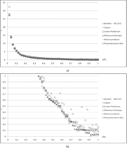
Estimation error  versus
  when
when  and
and  : a) global trend; b) zoom of the
  region.
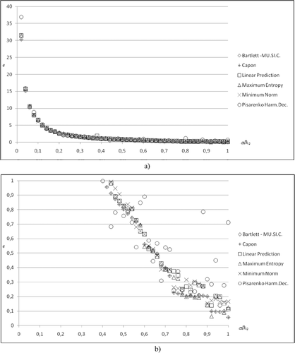
Estimation error  versus
  when
when  and
and  : a) global trend; b) zoom of the
  region.
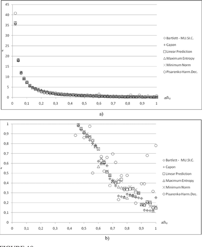
Estimation error  versus
  when
when  and
and  : a) global trend; b) zoom of the
  region.
In Fig. 7 it can be noticed that the estimation error is generally decreasing as radius  grows but it tends to increase in the proximity of the value
  . In this case, in fact, the distance between the receiving antenna and the centre of the object approaches
  , which is the far-zone limit of the sub-array previously specified. In Figs 8–10 it can be argued that the trend of
  versus
  becomes more regular as the windows size increases and simultaneously the radius of the smallest object that can be properly localized increases toward
  .
.
Furthermore, the Bartlett and multiple signals classification methods give the same values of  in most of the cases. As a general observation, we point out that they are, together with the maximum entropy, the methods that better localize the object.
In Table 5 some results concerning an object placed in a peripheral position compared with the array axis centre ( ), are presented. In particular we considered scenarios A and E of both the configurations studied in Tables 2 and 4.
It is clear that peripheral localization is affected by a higher estimation error when the object is placed in a vacuum, if compared with the results of Table 2. Instead, when the cylinder is buried in the medium with  , the procedure seems to be more robust to a position offset. It has to be considered that, in this second case, all the dimensions (distance between antenna sensors, distance
  and radius
  ) are reduced by a factor
  so that the object is closer to the array axis than in the vacuum case. Moreover, the host medium is supposed to be homogeneous and lossless: if losses were considered, the localization would be more sensitive to the position offset.
CONCLUSION
An algorithm has been presented that can detect and localize an object in the proximity of a linear array of receiving antennas, this distance could be referred to as the far-field limit of the sub-arrays in which the array is partitioned. The adopted sub-array processing technique has low computational complexity, is easy and affordable to use. Several directions of arrival estimation algorithms have been implemented and employed.
The described procedure has been applied to numerous test scenarios involving a perfectly-conducting circular cylinder having radius not larger than a wavelength. It shows good capability in estimating the scatterer position, either when the cylinder is set in a vacuum or inside a dielectric half-space. In particular we checked the procedure performances varying the geometrical parameters and the size of the windows used to discretize and probe the region of interest. The numerical results show that the Pisarenko harmonic decomposition method gives an average error greater than the other directions of arrival techniques independently from the windows size. The Linear Prediction algorithm presents worst performances when the windows are small, showing a behaviour similar to the other methods as the windows size is increased.
Furthermore, several scenarios have been considered, with the object in a peripheral position with respect to the array axis, both when the cylinder is settled in a vacuum and in a dielectric medium. In particular, in this second case, the procedure shows good robustness to a positional offset of the target.
We intend to consider a more realistic scenario, with the object buried in a lossy medium under a rough surface. We also plan to study the effect on the localization error of different subdivisions of the array in sub-arrays.
Moreover, we look forward to estimate also the scatterer dimension and to apply our sub-array processing strategy in multiple objects localization.


 is the pseudospectrum having the following expression (Burg
