Measuring Group Differences in High-Dimensional Choices: Method and Application to Congressional Speech
Abstract
We study the problem of measuring group differences in choices when the dimensionality of the choice set is large. We show that standard approaches suffer from a severe finite-sample bias, and we propose an estimator that applies recent advances in machine learning to address this bias. We apply this method to measure trends in the partisanship of congressional speech from 1873 to 2016, defining partisanship to be the ease with which an observer could infer a congressperson's party from a single utterance. Our estimates imply that partisanship is far greater in recent years than in the past, and that it increased sharply in the early 1990s after remaining low and relatively constant over the preceding century.
1 Introduction
In many settings, researchers seek to measure differences in the choices made by different groups, and the way such differences evolve over time. Examples include measuring the extent of racial segregation in residential choices (Reardon and Firebaugh (2002)), of partisanship in digital media consumption (Gentzkow and Shapiro (2011), Flaxman, Goel, and Rao (2016)), of geographic differences in treatment choices of physicians (Chandra, Cutler, and Song (2012)), and of differences between demographic groups in survey responses (Bertrand and Kamenica (2018)). We consider the problem of measuring such differences in settings where the dimensionality of the choice set is large—that is, where the number of possible choices is large relative to the number of actual choices observed. We show that in such settings, standard approaches suffer from a severe finite-sample bias, and we propose methods based on recent advances in machine learning that address this bias in a way that is computationally tractable with large-scale data.
Our approach is motivated by a specific application: measuring trends in party differences in political speech. It is widely apparent that America's two political parties speak different languages.1 Partisan differences in language diffuse into media coverage (Gentzkow and Shapiro (2010), Martin and Yurukoglu (2017)) and other domains of public discourse (Greenstein and Zhu (2012), Jensen, Naidu, Kaplan, and Wilse-Samson (2012)), and partisan framing has been shown to have large effects on public opinion (Nelson, Clawson, and Oxley (1997), Graetz and Shapiro (2006), Chong and Druckman (2007)).
Our main question of interest is to what extent the party differences in speech that we observe today are a new phenomenon. One can easily find examples of politically charged terms in America's distant past.2 Yet the magnitude of the differences between parties, the deliberate strategic choices that seem to underlie them, and the expanding role of consultants, focus groups, and polls (Bai (2005), Luntz (2006), Issenberg (2012)) suggest that the partisan differences in language that we see today might represent a consequential change (Lakoff (2003)). If the two parties speak more differently today than in the past, these divisions could be contributing to deeper polarization in Congress and cross-party animus in the broader public.
We use data on the text of speeches in the U.S. Congress from 1873 to 2016 to quantify the magnitude of partisan differences in speech, and to characterize the way these differences have evolved over time. We specify a multinomial model of speech with choice probabilities that vary by party. We measure partisan differences in speech in a given session of Congress by the ease with which an observer who knows the model could guess a speaker's party based solely on the speaker's choice of a single phrase. We call this measure partisanship for short.
To compute an accurate estimate of partisanship, we must grapple with two methodological challenges. The first is the finite-sample bias mentioned above. The bias arises because the number of phrases a speaker could choose is large relative to the total amount of speech we observe, so many phrases are said mostly by one party or the other purely by chance. Naive estimators interpret such differences as evidence of partisanship, leading to a bias we show can be many orders of magnitude larger than the true signal in the data. Second, although our model takes a convenient multinomial logit form, the large number of choices and parameters makes standard approaches to estimation computationally infeasible.
We use two estimation approaches to address these challenges. The first is a leave-out estimator that addresses the main source of finite-sample bias while allowing for simple inspection of the data. The second, our preferred estimator, uses an  or lasso-type penalty on key model parameters to control bias, and a Poisson approximation to the multinomial logit likelihood to permit distributed computing. A permutation test and an out-of-sample validation both suggest that any bias that remains in these estimates is dramatically lower than in standard approaches, and small relative to the true variation in partisanship over time.
We find that the partisanship of language has exploded in recent decades, reaching an unprecedented level. From 1873 to the early 1990s, partisanship was nearly constant and fairly small in magnitude: in the 43rd session of Congress (1873–1875), the probability of correctly guessing a speaker's party based on a one-minute speech was 54 percent; by the 101st session (1989–1990), this figure had increased to 57 percent. Beginning with the congressional election of 1994, partisanship turned sharply upward, with the probability of guessing correctly based on a one-minute speech climbing to 73 percent by the 110th session (2007–2009). Methods that do not correct for finite-sample bias, including the maximum likelihood estimator of our model, instead imply that partisanship is no higher today than in the past.
We unpack the recent increase in partisanship along a number of dimensions. The most partisan phrases in each period—defined as those phrases most diagnostic of the speaker's party—align well with the issues emphasized in party platforms and, in recent years, include well-known partisan phrases such as “death tax” and “estate tax.” Manually classifying phrases into substantive topics shows that the increase in partisanship is due more to changes in the language used to discuss a given topic (e.g., “death tax” vs. “estate tax”) than to changes in the topics parties emphasize (e.g., Republicans focusing more on taxes and Democrats focusing more on labor issues).
While we cannot definitively say why partisanship of language increased when it did, the evidence points to innovation in political persuasion as a proximate cause. The 1994 inflection point in our series coincides precisely with the Republican takeover of Congress led by Newt Gingrich, under a platform called the Contract with America (Gingrich and Armey (1994)). This election is widely considered a watershed moment in political marketing, with consultants such as Frank Luntz applying novel techniques to identify effective language and disseminate it to candidates (Lakoff (2004), Luntz (2004), Bai (2005)). We also discuss related changes such as the expansion of cable television coverage that may have provided further incentives for linguistic innovation.
This discussion highlights that partisanship of speech as we define it is a distinct phenomenon from other inter-party differences. In particular, the large body of work building on the ideal point model of Poole and Rosenthal (1985) finds that inter-party differences in roll-call voting fell from the late nineteenth to the mid-twentieth century, and have since steadily increased (McCarty, Poole, and Rosenthal (2015)). These dynamics are very different from those we observe in speech, consistent with our expectation that speech and roll-call votes respond to different incentives and constraints, and suggesting that the analysis of speech may reveal aspects of the political landscape that are not apparent from the analysis of roll-call votes.
We build on methods developed by Taddy (2013, 2015). Many aspects of the current paper, including our proposed leave-out estimator, our approaches to validation and inference, and the covariate specification of our model, are novel with respect to that prior work. Most importantly, Taddy (2013, 2015) made no attempt to define or quantify the divergence in language between groups either at a point in time or over time, nor did he discuss the finite-sample biases that arise in doing so. Our paper also relates to other work on measuring document partisanship, including Laver, Benoit, and Garry (2003), Groseclose and Milyo (2005), Gentzkow and Shapiro (2010), Kim, Londregan, and Ratkovic (2018), and Yan, Das, Lavoie, Li, and Sinclair (2018).3
Our paper contributes a recipe for using statistical predictability in a probability model of speech as a metric of differences in partisan language between groups. Jensen et al. (2012) used text from the Congressional Record to characterize party differences in language from the late nineteenth century to the present. Their index, which is based on the observed correlation of phrases with party labels, implies that partisanship has been rising recently but was similarly high in the past. We apply a different method that addresses finite-sample bias and leads to substantially different conclusions. Lauderdale and Herzog (2016) specified a generative hierarchical model of floor debates and estimated the model on speech data from the Irish Dail and the U.S. Senate. Studying the U.S. Senate from 1995 to 2014, they found that party differences in speech have increased faster than party differences in roll-call voting. Peterson and Spirling (2018) studied trends in the partisanship of speech in the UK House of Commons. In contrast to Lauderdale and Herzog's (2016) analysis (and ours), Peterson and Spirling (2018) did not specify a generative model of speech. Instead, Peterson and Spirling (2018) measured partisanship using the predictive accuracy of several machine-learning algorithms. They cited our article to justify using randomization tests to check for spurious trends in their measure. These tests (Peterson and Spirling (2018), Supplemental Material Appendix C) show that their measure implies significant and time-varying partisanship even in fictitious data in which speech patterns are independent of party.
The recipe that we develop can be applied to a broad class of problems in which the goal is to characterize group differences in high-dimensional choices. A prominent example is the measurement of residential segregation (e.g., Reardon and Firebaugh (2002)), where the groups might be defined by race or ethnicity and the choices might be neighborhoods or schools. The finite-sample bias that we highlight has been noted in that context by Cortese, Falk, and Cohen (1976) and addressed by benchmarking against random allocation (Carrington and Troske (1997)), applying asymptotic or bootstrap bias corrections (Allen, Burgess, Davidson, and Windmeijer (2015)), and estimating mixture models (Rathelot (2012), D'Haultfœuille and Rathelot (2017)).4 Recent work has derived axiomatic foundations for segregation measures (Echenique and Fryer (2007), Frankel and Volij (2011)), asking which measures of segregation satisfy certain properties.5 Instead, our approach is to specify a generative model of the data and to measure group differences using objects that have a well-defined meaning in the context of the model.6 In the body of the paper, we note some formal connections to the literature on residential segregation, and in an earlier draft, we pursue a detailed application to trends in residential segregation by political affiliation (Gentzkow, Shapiro, and Taddy (2017)).
2 Congressional Speech Data
Our primary data source is the text of the United States Congressional Record (hereafter, the Record) from the 43rd Congress to the 114th Congress. We obtain digital text from HeinOnline, who performed optical character recognition (OCR) on scanned print volumes. The Record is a “substantially verbatim” record of speech on the floor of Congress (Amer (1993)). We exclude Extensions of Remarks, which are used to print unspoken additions by members of the House that are not germane to the day's proceedings.7
The modern Record is issued in a daily edition, printed at the end of each day that Congress is in session, and in a bound edition that collects the content for an entire Congress. These editions differ in formatting and in some minor elements of content (Amer (1993)). Our data contain bound editions for the 43rd to 111th Congresses, and daily editions for the 97th to 114th Congresses. We use the bound edition in the sessions where it is available and the daily edition thereafter. The Supplemental Material (Gentzkow, Shapiro, and Taddy (2019)) shows results from an alternative data build that uses the bound edition through the 96th Congress and the daily edition thereafter.
We use an automated script to parse the raw text into individual speeches. Beginnings of speeches are demarcated in the Record by speaker names, usually in all caps (e.g., “Mr. ALLEN of Illinois.”). We determine the identity of each speaker using a combination of manual and automated procedures, and append data on the state, chamber, and gender of each member from historical sources.8 We exclude any speaker who is not a Republican or a Democrat, speakers who are identified by office rather than name, non-voting delegates, and speakers whose identities we cannot determine.9 The Supplemental Material presents the results of a manual audit of the reliability of our parsing.
The input to our main analysis is a matrix  whose rows correspond to speakers and whose columns correspond to distinct two-word phrases or bigrams (hereafter, simply “phrases”). An element
  thus gives the number of times speaker i has spoken phrase j in session (Congress) t. To create these counts, we first perform the following pre-processing steps: (i) delete hyphens and apostrophes; (ii) replace all other punctuation with spaces; (iii) remove non-spoken parenthetical insertions; (iv) drop a list of extremely common words;10 and (v) reduce words to their stems according to the Porter2 stemming algorithm (Porter (2009)). We then drop phrases that are likely to be procedural or have low semantic meaning according to criteria we define in the Supplemental Material. Finally, we restrict attention to phrases spoken at least 10 times in at least one session, spoken in at least 10 unique speaker-sessions, and spoken at least 100 times across all sessions. The Supplemental Material presents results from a sample in which we tighten each of these restrictions by 10 percent. The Supplemental Material also presents results from an alternative construction of
  containing counts of three-word phrases or trigrams.
The decision to represent text as a matrix of phrase counts is fairly common in text analysis, as is the decision to reduce the dimensionality of the data by removing word stems and non-word content (Gentzkow, Kelly, and Taddy (Forthcoming)). We remove procedural phrases because they appear frequently and their use is likely not informative about the inter-party differences that we wish to measure (Gentzkow and Shapiro (2010)). We remove infrequently used phrases to economize on computation (Gentzkow, Kelly, and Taddy (Forthcoming)).
The resulting vocabulary contains 508,352 unique phrases spoken a total of 287 million times by 7732 unique speakers. We analyze data at the level of the speaker-session, of which there are 36,161. The Supplemental Material reports additional summary statistics for our estimation sample and vocabulary.
We identify 22 substantive topics based on our knowledge of the Record. We associate each topic with a non-mutually exclusive subset of the vocabulary. To do this, we begin by grouping a set of partisan phrases into the 22 topics (e.g., taxes, defense, etc.). For each topic, we form a set of keywords by (i) selecting relevant words from the associated partisan phrases and (ii) manually adding other topical words. Finally, we identify all phrases in the vocabulary that include one of the topic keywords, are used more frequently than a topic-specific occurrence threshold, and are not obvious false matches. The Supplemental Material lists, for each topic, the keywords, the occurrence threshold, and a random sample of included and excluded phrases.
3 Model and Measure of Partisanship
3.1 Model of Speech
 of phrase counts for speaker i, which we assume comes from a multinomial distribution
 (1)
(1) denoting the total amount of speech by speaker i in session t,
  denoting the party affiliation of speaker i,
  denoting a K-vector of (possibly time-varying) speaker characteristics, and
  denoting the vector of choice probabilities. We let
  and
and  denote the set of Republicans and Democrats, respectively, active in session t. The speech-generating process is fully characterized by the verbosity
  and the probability
  of speaking each phrase.
 (2)
(2) is a scalar parameter capturing the baseline popularity of phrase j in session t,
  is a K-vector capturing the effect of characteristics
  on the propensity to use phrase j in session t, and
  is a scalar parameter capturing the effect of party affiliation on the propensity to use phrase j in session t. If
  , any phrase probabilities
  can be represented with appropriate choice of parameters in equation (2).
The model in (1) and (2) is restrictive, and it ignores many important aspects of speech. For example, it implies that the propensity to use a given phrase is not related to other phrases used by speaker i in session t, and need not be affected by the speaker's verbosity  . We adopt this model because it is tractable and has proved useful in extracting meaning from text in many related contexts (Groseclose and Milyo (2005), Taddy (2013, 2015)).
The model also implies that speaker identities matter only through party affiliation  and the characteristics
  . Specification of
  is therefore important for our analysis. We consider specifications of
  with different sets of observable characteristics, as well as a specification with unobserved speaker characteristics (i.e., speaker random effects).
We assume throughout that if a phrase (or set of phrases) is excluded from the choice set, the relative frequencies of the remaining phrases are unchanged. We use this assumption in Sections 6 and 7 to compute average partisanship for interesting subsets of the full vocabulary. This assumption encodes the independence of irrelevant alternatives familiar from other applications of the multinomial logit model. It is a restrictive assumption, as some phrases are clearly better substitutes than others, but it provides a useful benchmark for analysis absent a method for estimating flexible substitution patterns in a large vocabulary.
3.2 Measure of Partisanship
For given characteristics  , we define partisanship of speech to be the divergence between
  and
and  . When these vectors are close, Republicans and Democrats speak similarly and we say that partisanship is low. When these vectors are far from each other, the parties speak differently and we say that partisanship is high.
We choose a particular measure of this divergence that has a clear interpretation in the context of our model: the posterior probability that an observer with a neutral prior expects to assign to a speaker's true party after hearing the speaker utter a single phrase.
Definition.The partisanship of speech at  is
is
 (3)
(3) (4)
(4) (5)
(5)To understand these definitions, note that  is the posterior belief that an observer with a neutral prior assigns to a speaker being Republican if the speaker chooses phrase j in session t and has characteristics
  . Partisanship
  averages
  over the possible parties and phrases: if the speaker is a Republican (which occurs with probability
  ), the probability of a given phrase j is
  and the probability assigned to the true party after hearing j is
  ; if the speaker is a Democrat, these probabilities are
  and
and  , respectively. Average partisanship
  , which is our target for estimation, averages
  over the characteristics
  of speakers active in session t. Average partisanship is defined with respect to a given vocabulary of J phrases.
There are many possible measures of the divergence between  and
and  . We show in the Supplemental Material that the time series of partisanship looks qualitatively similar if we replace our partisanship measure with either the Euclidean distance between
  and
and  or the implied mutual information between party and phrase choice, though the series for Euclidean distance is noisier.
Partisanship is closely related to the isolation index, a common index of residential segregation (White (1986), Cutler, Glaeser, and Vigdor (1999)).11 Frankel and Volij (2011) characterized a large set of segregation indices based on a set of ordinal axioms. Ignoring covariates  , our measure satisfies six of these axioms: Non-triviality, Continuity, Scale Invariance, Symmetry, Composition Invariance, and the School Division Property. It fails to satisfy one axiom: Independence.12
Average partisanship  summarizes how well an observer can predict a hypothetical speaker's party given a single realization and knowledge of the true model. This is distinct from the question of how well an econometrician can predict a given speaker's party in a given sample of text.
4 Estimation, Inference, and Validation
4.1 Plug-in Estimators
Maximum likelihood estimation is straightforward in our context. Ignoring covariates  , the maximum likelihood estimator (MLE) can be computed by plugging in empirical analogues for the terms that appear in equation (3).
 be the empirical phrase frequencies for speaker i. Let
  be the empirical phrase frequencies for party P, and let
  , excluding from the choice set any phrases that are not spoken in session t. Then the MLE of
  when
when  is
is
 (6)
(6)An important theme of our paper is that this and related estimators can be severely biased in finite samples even if  . Intuitively, partisanship will be high when the dispersion of the posteriors
  is large—that is, when some phrases are spoken far more by Republicans and others are spoken far more by Democrats. The MLE estimates the
  using their sample analogues
  . However, sampling error will tend to increase the dispersion of the
  relative to the dispersion of the true
  . When the number of phrases is large relative to the volume of speech observed, many phrases will be spoken only a handful of times, and so may be spoken mainly by Republicans (
 ) or mainly by Democrats (
 ) by chance even if the true choice probabilities do not differ by party.
 is a convex function of
  and
and  , and so Jensen's inequality implies that it has a positive bias. We can also use the fact that
  to decompose the bias of a generic term
  as
as
 (7)
(7) is mechanically related to the sampling error in
  . Any positive residual in
  will increase both terms inside the covariance; any negative residual will do the reverse. The first term is also nonzero because
  is a nonlinear transformation of
  ,13 though this component of the bias tends to be small in practice.
The bias we highlight is not specific to the MLE, but will tend to arise for any measure of group differences that uses observed choices as a direct approximation of true choice probabilities. This is especially transparent if we measure the difference between  and
and  using a norm such as Euclidean distance: Jensen's inequality implies that for any norm
  ,
, 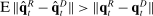 . Similar issues arise for the measure of Jensen et al. (2012), which is given by
 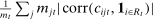 . If speech is independent of party (
 ) and verbosity is fixed, then the population value of
  is zero. But in any finite sample, the correlation will be nonzero with positive probability, so the measure may imply party differences even when speech is unrelated to party.
4.2 Leave-out Estimator
The first approach we propose to addressing this bias is a leave-out estimator that uses different samples to estimate  and
and  . This makes the errors in the former independent of the errors in the latter by construction, and so eliminates the second bias term in equation (7).
 (8)
(8) is the analogue of
  computed from the speech of all speakers other than i.14 This estimator is biased for
  , even if
  , because of the first term in equation (7), but we expect (and find) that this bias is small in practice.
The leave-out estimator is simple to compute and provides a direct look at the patterns in the data. It also has important limitations. In particular, it does not allow us to incorporate covariates. In addition, it does not recover the underlying parameters of the model and so does not directly provide estimates of objects such as the most partisan phrases, which we rely on heavily in our application.
4.3 Penalized Estimator
 of equation (2) by minimization of the following penalized objective function:
 (9)
(9) of
of  by substituting estimated parameters into the probability objects in equation (5).
Because partisanship is defined as a function of the characteristics  , the choice of characteristics to include in the model affects our target for estimation. We wish to include those characteristics that are likely to be related both to party and to speech but whose relationship with speech would not generally be thought of as a manifestation of party differences. A leading example of such a confound is geographic region: speakers from different parts of the country will tend to come from different parties and to use different phrases, but regional differences in language would not generally be thought of as a manifestation of party differences.
In our baseline specification,  consists of indicators for state, chamber, gender, Census region, and whether the party is in the majority for the entirety of the session. The coefficients
  on these attributes are static in time (i.e.,
  ) except for those on Census region, which are allowed to vary freely across sessions to allow more flexibly for regional variation in speech. The Supplemental Material shows results from a specification in which
  includes unobserved speaker-level preference shocks (i.e., speaker random effects), from a specification in which
  includes no covariates, and from a specification in which
  includes several additional covariates.
The minimand in (9) encodes two key decisions. First, we approximate the likelihood of our multinomial logit model with the likelihood of a Poisson model (Palmgren (1981), Baker (1994), Taddy (2015)), where  , and we use the plug-in estimate
  of the parameter
  . Because the Poisson and the multinomial logit share the same conditional likelihood
  , their MLEs coincide when
  is the MLE. Although our plug-in is not the MLE, Taddy (2015) showed that our approach often performs well in related settings. In the Supplemental Material, we show that our estimator performs well on data simulated from the multinomial logit model.
We adopt the Poisson approximation because, fixing  , the likelihood of the Poisson is separable across phrases. This feature allows us to use distributed computing to estimate the model parameters (Taddy (2015)). Without the Poisson approximation, computation of our estimator would be infeasible due to the cost of repeatedly calculating the denominator of the logit choice probabilities.
The second key decision is the use of an  penalty
  , which imposes sparsity on the party loadings and shrinks them toward zero (Tibshirani (1996)). Sparsity and shrinkage limit the effect of sampling error on the dispersion of the estimated posteriors
  , which is the source of the bias in
  . We determine the penalties
  by regularization path estimation, first finding
  large enough so that
  is estimated to be 0, and then incrementally decreasing
  and updating parameter estimates accordingly. An attractive computational property of this approach is that the coefficient estimates change smoothly along the path of penalties, so each segment's solution acts as a hot-start for the next segment and the optimizations are fast to solve. We then choose the value of
  that minimizes a Bayesian Information Criterion.15 The Supplemental Material reports a qualitatively similar time series of partisanship when we use 5- or 10-fold cross-validation to select the
  that minimizes average out-of-sample deviance.
We also impose a minimal penalty of  on the phrase-specific intercepts
  and the covariate coefficients
  . We do this to handle the fact that some combinations of data and covariate design do not have an MLE in the Poisson model (Haberman (1973), Santos Silva and Tenreyro (2010)). A small penalty allows us to achieve numerical convergence while still treating the covariates in a flexible way.16
4.4 Inference
For all of our main results, we perform inference via subsampling. We draw without replacement 100 random subsets of size equal to one-tenth the number of speakers (up to integer restrictions) and re-estimate on each subset. We report confidence intervals based on the distribution of the estimator across these subsets, under the assumption of  convergence. We center these confidence intervals around the estimated series and report uncentered bias-corrected confidence intervals for our main estimator in the Supplemental Material.
Politis, Romano, and Wolf (1999, Theorem 2.2.1) showed that this procedure yields valid confidence intervals under the assumption that the distribution of the estimator converges weakly to some non-degenerate distribution at a  rate. In the Appendix, we extend a result of Knight and Fu (2000) to show that this property holds, with fixed vocabulary and a suitable rate condition on the penalty, for the penalized maximum likelihood estimator of our multinomial logit model. This is the estimator that we approximate with the Poisson distribution in equation (9). Though we do not pursue formal results for the case where the vocabulary grows with the sample size, we note that such asymptotics might better approximate the finite-sample behavior of our estimators.
In the Supplemental Material, we report the results of several exercises designed to probe the accuracy of our confidence intervals. First, we consider three alternative subsampling strategies: (i) doubling the number of speakers in each subsample, (ii) using 10 non-overlapping subsamples rather than 100 overlapping subsamples, and (iii) using 5 non-overlapping subsamples. Second, we compute confidence intervals based on a parametric bootstrap, repeatedly simulating data from our estimated model and re-estimating the model on the simulated data. Third, we compute confidence intervals using a sample-splitting procedure that uses one half of the model to perform variable selection and then estimates the selected model with minimal penalty across repeated bootstrap replicates on the second half of the sample. All of these procedures yield qualitatively similar conclusions. Note that we do not report results for a standard nonparametric bootstrap; the standard nonparametric bootstrap is known to be invalid for lasso regression (Chatterjee and Lahiri (2011)).
4.5 Validation
As usual with nonlinear models, none of the estimators proposed here are exactly unbiased in finite samples. Our goal is to reduce bias to the point that it is dominated by the signal in the data. We gauge our success in three main ways.
First, we consider a permutation test in which we randomly reassign parties to speakers and then re-estimate each measure on the resulting data. In this “random” series,  by construction, so the true value of
  is equal to
  in all years. Thus the random series for an unbiased estimator of
  has expected value
  in each session t, and the deviation from
  provides a valid measure of bias under the permutation.
Second, in the Supplemental Material we present results from exercises in which we apply our estimators to two types of simulated data. The first exercise is a Monte Carlo in which we simulate data from our estimated model. The second exercise is a falsification test in which we simulate data from a model in which  and
and  (and hence partisanship) are constant over time but verbosity
  is allowed to follow its empirical distribution.
Third, we perform an out-of-sample validation in which our hypothetical observer learns the partisanship of phrases from one sample of speech and attempts to predict the party of speakers in another. In particular, we divide the sample of speakers into five mutually exclusive partitions. For each partition k and each estimator, we estimate the  terms in equation (3) using the given estimator on the sample excluding the kth partition, and the
  and
and  terms using their empirical frequencies within the kth partition. We then average the estimates across partitions and compare to our in-sample estimates.
5 Main Results
Figure 1 presents the time series of the maximum likelihood estimator  of our model, and of the index reported by Jensen et al. (2012) computed from their publicly available data.17 Panel A shows that the random series for
  is far from
  , indicating that the bias in the MLE is severe in practice. Variation over time in the magnitude of the bias dominates the series, leading the random series and the real series to be highly correlated. Taking the MLE at face value, we would conclude that language was much more partisan in the past and that the upward trend in recent years is small by historical standards.

Average partisanship and polarization of speech, plug-in estimates. Notes: Panel A plots the average partisanship series from the maximum likelihood estimator  defined in Section 4.1. “Real” series is from actual data; “random” series is from hypothetical data in which each speaker's party is randomly assigned with the probability that the speaker is Republican equal to the average share of speakers who are Republican in the sessions in which the speaker is active. The shaded region around each series represents a pointwise confidence interval obtained via subsampling (Politis, Romano, and Wolf (1999)). Specifically, we randomly draw speakers without replacement to create 100 subsamples each containing (up to integer restrictions) one-tenth of all speakers and, for each subsample k, we compute the MLE estimate
  . Let τk be the number of speakers in the kth subsample and let τ be the number of speakers in the full sample. Then the confidence interval on the MLE is
  , where
  is the bth order statistic of
  . Panel B plots the standardized measure of polarization from Jensen et al. (2012). Polarization in session t is defined as ∑j(mjt|ρjt|/∑lmlt), where
 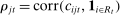 ; the series is standardized by subtracting its mean and dividing by its standard deviation. “Real” series reproduces the polarization series in Figure 3B of Jensen et al. (2012) using the replication data for that paper; “random” series uses the same data but randomly assigns each speaker's party with the probability that the speaker is Republican equal to the average share of speakers who are Republican in the sessions in which the speaker is active.
Because bias is a finite-sample property, it is natural to expect that the severity of the bias in  in a given session t depends on the amount of speech—that is, on the verbosities
  of speakers in that session. The Supplemental Material shows that this is indeed the case: a first-order approximation to the bias in
  as a function of verbosity follows a similar path to the random series in Panel A of Figure 1, and the dynamics of
  are similar to those in the real series when we allow verbosity to follow its empirical distribution but fix phrase frequencies
  at those observed in a particular session
  . The Supplemental Material also shows that while the severity of the bias falls as we exclude less frequently spoken phrases, very severe sample restrictions are needed to control bias, and a significant time-varying bias remains even when we exclude 99 percent of phrases from our calculations.18
Panel B of Figure 1 shows that the Jensen et al. (2012) polarization measure behaves similarly to the MLE. The plot for the real series replicates the published version. The random series is far from 0, and the real and random series both trend downward in the first part of the sample period. Jensen et al. (2012) concluded that polarization has been increasing recently, but that it was as high or higher in earlier years. The results in Panel B suggest that the second part of this conclusion could be an artifact of the finite-sample mechanics of their index.
Figure 2 presents our main estimates. Panel A shows the leave-out estimator  . The random series suggests that the leave-out correction largely purges the estimator of bias: the series is close to
  throughout the period.

Average partisanship of speech, leave-out and penalized estimates. Notes: Panel A plots the average partisanship series from the leave-out estimator  defined in Section 4.2. Panel B plots the average partisanship series from our preferred penalized estimator
  defined in Section 4.3. In each plot, the “real” series is from actual data and the “random” series is from hypothetical data in which each speaker's party is randomly assigned with the probability that the speaker is Republican equal to the average share of speakers who are Republican in the sessions in which the speaker is active. The shaded region around each series represents a pointwise confidence interval obtained via subsampling (Politis, Romano, and Wolf (1999)). Specifically, we randomly draw speakers without replacement to create 100 subsamples each containing (up to integer restrictions) one-tenth of all speakers and, for each subsample k, we compute the leave-out estimate
  and the penalized estimate
  . Let τk be the number of speakers in the kth subsample and let τ be the number of speakers in the full sample. Then the confidence interval on the leave-out estimator is
  , where
  is the bth order statistic of
  . The confidence interval on the penalized estimator is
  , where
  is the bth order statistic of
  .
.
Panel B presents our preferred penalized estimator, including controls for covariates  . Estimates for the random series indicate minimal bias. The Supplemental Material shows that the use of regularization is the key to the performance of this estimator: imposing only a minimal penalty (i.e., setting
  ) leads, as expected, to behavior similar to that of the MLE. The Supplemental Material also shows that, in contrast to the MLE, the dynamics of our proposed estimators cannot be explained by changes in verbosity over time.
Looking at the data through the sharper lens of the leave-out and penalized estimators reveals that partisanship was low and relatively constant until the early 1990s, then exploded, reaching unprecedented heights in recent years. This is a dramatically different picture than one would infer from the MLE or the Jensen et al. (2012) series. The sharp increase in partisanship is much larger than the width of the subsampling confidence intervals.
The increase is also large in magnitude. Recall that average partisanship is the posterior that a neutral observer expects to assign to a speaker's true party after hearing a single phrase. Figure 3 extends this concept to show the expected posterior for speeches of various lengths. An average one-minute speech in our data contains around 33 phrases (after pre-processing). In 1874, an observer hearing such a speech would expect to have a posterior of around 0.54 on the speaker's true party, only slightly above the prior of 0.5. By 1990, this value increased slightly to 0.57. Between 1990 and 2008, however, it leaped up to 0.73.

Informativeness of speech by speech length and session. Notes: For each speaker i and session t, we calculate, given characteristics  , the expected posterior that an observer with a neutral prior would place on a speaker's true party after hearing a given number of phrases drawn according to our preferred specification in Panel B of Figure 2. We perform this calculation by Monte Carlo simulation and plot the average across speakers for each given session and length of speech. The vertical line shows the average number of phrases in one minute of speech. We calculate this by sampling 95 morning-hour debate speeches across the second session of the 111th Congress and the first session of the 114th Congress. We use https://www.c-span.org/ to calculate the time-length of each speech and to obtain the text of the Congressional Record associated with each speech, from which we obtain the count of phrases in our main vocabulary following the procedure outlined in Section 2. The vertical line shows the average ratio, across speeches, of the phrase count to the number of minutes of speech.
Figure 4 presents the out-of-sample validation exercise described in Section 4.5 for the MLE, leave-out, and penalized estimators. We find that the MLE greatly overstates partisanship relative to its out-of-sample counterpart. Based on the in-sample estimate, one would expect an observer to be able to infer a speaker's party with considerable accuracy, but when tested out of sample, the predictive power turns out to be vastly overstated. In contrast, both the leave-out and penalized estimators achieve values quite close to their out-of-sample counterparts, as desired.

Out-of-sample validation. Notes: Let  ,
,  , and
, and  be functions estimated using the maximum likelihood estimator on a sample of speakers
  . Let
. Let  ,
,  , and
, and  be functions estimated using our preferred penalized estimator on sample
  and evaluated at the sample mean of the covariates in session t and sample
  . Let
. Let  be the full sample of speakers and let
  for k = 1,…,K denote K = 5 mutually exclusive partitions (“folds”) of
  , with
  denoting the sample excluding the kth fold. For P ∈ {R,D}, denote
  and
and  . The lines labeled “in-sample” in Panels A, B, and C present the in-sample estimated partisanship using the maximum likelihood estimator, leave-out estimator, and our preferred penalized estimator. These are the same as in Figure 1 and Figure 2. The line labeled “out-of-sample” in Panel A presents the average, across folds, of the out-of-sample estimated partisanship using the maximum likelihood estimator:
  . The line labeled “out-of-sample” in Panel B presents the average, across folds, of the out-of-sample estimated partisanship using the leave-out estimator:
  , which is derived by replacing
  in the in-sample leave-out with its counterpart calculated on the sample excluding the kth fold. The line labeled “out-of-sample” in Panel C presents the average, across folds, of the out-of-sample estimated partisanship using our preferred penalized estimator:
  .
.
In Figure 2, the penalized estimates in Panel B imply lower partisanship than the leave-out estimates in Panel A. Sampling experiments in the Supplemental Material show that the bias in the leave-out estimator is slightly positive, likely due to excluding controls for covariates, and that the bias in the penalized estimator is negative, possibly due to conservative overpenalization.
The Supplemental Material presents a range of alternative series based on variants of our baseline model, estimator, and sample. Removing covariates leads to greater estimated partisanship, while adding more controls or speaker random effects leads to lower estimated partisanship, though all of these variants imply a large rise in partisanship following the 1990s. Dropping the South from the sample does not meaningfully change the estimates, nor does excluding data from early decades. Using only the early decades or holding constant the number of congresspeople in each session somewhat increases our estimates of partisanship and bias, leaving the difference between the real and random series in line with our preferred estimates.
6 Unpacking Partisanship
6.1 Partisan Phrases
 is Republican is
  . If, unbeknownst to the observer, phrase j is removed from the vocabulary, the change in the expected posterior is

 of phrase j in session t to be the average of this value across all active speakers i in session t. This measure has both direction and magnitude: positive numbers are Republican phrases, negative numbers are Democratic phrases, and the absolute value gives the magnitude of partisanship.
Table I lists the ten most partisan phrases in every tenth session plus the most recent session. The Supplemental Material shows the list for all sessions. These lists illustrate the underlying variation driving our measure, and give a sense of how partisan speech has changed over time. In the Supplemental Material, we argue in detail that the top phrases in each of these sessions align closely with the policy positions and narrative strategies of the parties, confirming that our measure is indeed picking up partisanship rather than some other dimension that happens to be correlated with it. In this section, we highlight a few illustrative examples.
|
Session 50 (1887–1888) |
Session 60 (1907–1908) |
||||||||||
|
Republican |
|
|
Democratic |
|
|
Republican |
|
|
Democratic |
|
|
|
sixth street |
22 |
0 |
cutleri compani |
0 |
72 |
postal save |
39 |
3 |
canal zone |
18 |
66 |
|
union soldier |
33 |
13 |
labor cost |
11 |
37 |
census offic |
31 |
2 |
also petit |
0 |
47 |
|
color men |
27 |
10 |
increas duti |
11 |
34 |
reserv balanc |
36 |
12 |
standard oil |
4 |
25 |
|
railroad compani |
85 |
70 |
cent ad |
35 |
54 |
war depart |
62 |
39 |
indirect contempt |
0 |
19 |
|
great britain |
121 |
107 |
public domain |
20 |
39 |
secretari navi |
62 |
39 |
bureau corpor |
5 |
24 |
|
confeder soldier |
18 |
4 |
ad valorem |
61 |
78 |
secretari agricultur |
58 |
36 |
panama canal |
23 |
41 |
|
other citizen |
13 |
0 |
feder court |
11 |
25 |
pay pension |
20 |
2 |
nation govern |
12 |
30 |
|
much get |
12 |
1 |
high protect |
6 |
18 |
boat compani |
24 |
8 |
coal mine |
9 |
27 |
|
paper claim |
9 |
0 |
tariff tax |
11 |
23 |
twelfth census |
14 |
0 |
revis tariff |
8 |
26 |
|
sugar trust |
16 |
7 |
high tariff |
6 |
16 |
forestri servic |
20 |
7 |
feet lake |
0 |
17 |
|
Session 70 (1927–1928) |
Session 80 (1947–1948) |
||||||||||
|
Republican |
|
|
Democratic |
|
|
Republican |
|
|
Democratic |
|
|
|
war depart |
97 |
63 |
pension also |
0 |
163 |
depart agricultur |
67 |
31 |
unit nation |
119 |
183 |
|
take care |
105 |
72 |
american peopl |
51 |
91 |
foreign countri |
49 |
22 |
calumet region |
0 |
30 |
|
foreign countri |
54 |
28 |
radio commiss |
8 |
44 |
steam plant |
34 |
7 |
concili servic |
3 |
31 |
|
muscl shoal |
97 |
71 |
spoken drama |
0 |
30 |
coast guard |
34 |
9 |
labor standard |
16 |
41 |
|
steam plant |
25 |
3 |
civil war |
27 |
54 |
state depart |
117 |
93 |
depart labor |
24 |
46 |
|
nation guard |
39 |
18 |
trade commiss |
19 |
46 |
air forc |
88 |
69 |
collect bargain |
15 |
35 |
|
air corp |
32 |
12 |
feder trade |
19 |
45 |
stop communism |
22 |
3 |
standard act |
11 |
31 |
|
creek dam |
25 |
6 |
wave length |
6 |
25 |
nation debt |
43 |
25 |
polish peopl |
4 |
20 |
|
cove creek |
30 |
13 |
imperi valley |
12 |
28 |
pay roll |
34 |
17 |
budget estim |
22 |
38 |
|
american ship |
29 |
12 |
flowag right |
5 |
20 |
arm forc |
63 |
47 |
employ servic |
25 |
41 |
|
Session 90 (1967–1968) |
Session 100 (1987–1988) |
||||||||||
|
Republican |
|
|
Democratic |
|
|
Republican |
|
|
Democratic |
|
|
|
job corp |
35 |
20 |
human right |
7 |
44 |
judg bork |
226 |
14 |
persian gulf |
30 |
47 |
|
trust fund |
26 |
14 |
unit nation |
49 |
75 |
freedom fighter |
36 |
8 |
contra aid |
12 |
28 |
|
antelop island |
11 |
0 |
men women |
20 |
34 |
state depart |
59 |
35 |
star war |
1 |
14 |
|
treasuri depart |
23 |
12 |
world war |
57 |
71 |
human right |
101 |
78 |
central american |
17 |
30 |
|
federalaid highway |
13 |
2 |
feder reserv |
26 |
39 |
minimum wage |
37 |
19 |
aid contra |
17 |
30 |
|
tax credit |
21 |
11 |
million american |
15 |
27 |
reserv object |
23 |
8 |
nuclear wast |
14 |
27 |
|
state depart |
45 |
35 |
arm forc |
25 |
37 |
demand second |
13 |
1 |
american peopl |
97 |
109 |
|
oblig author |
14 |
4 |
high school |
19 |
30 |
tax increas |
20 |
10 |
interest rate |
24 |
35 |
|
highway program |
14 |
4 |
gun control |
10 |
22 |
pay rais |
21 |
11 |
presid budget |
11 |
21 |
|
invest act |
11 |
1 |
air pollut |
18 |
29 |
plant close |
37 |
28 |
feder reserv |
12 |
22 |
|
Session 110 (2007–2008) |
Session 114 (2015–2016) |
||||||||||
|
Republican |
|
|
Democratic |
|
|
Republican |
|
|
Democratic |
|
|
|
tax increas |
87 |
20 |
dog coalit |
0 |
90 |
american peopl |
327 |
205 |
homeland secur |
96 |
205 |
|
natur gas |
77 |
20 |
war iraq |
18 |
78 |
al qaeda |
50 |
7 |
climat chang |
23 |
94 |
|
reserv balanc |
147 |
105 |
african american |
6 |
62 |
men women |
123 |
83 |
gun violenc |
3 |
74 |
|
rais tax |
44 |
10 |
american peopl |
230 |
278 |
side aisl |
133 |
93 |
african american |
11 |
71 |
|
american energi |
34 |
3 |
oil compani |
20 |
65 |
human traffick |
60 |
26 |
vote right |
2 |
62 |
|
illeg immigr |
34 |
7 |
civil war |
17 |
45 |
colleagu support |
123 |
89 |
public health |
24 |
83 |
|
side aisl |
132 |
106 |
troop iraq |
11 |
39 |
religi freedom |
34 |
4 |
depart homeland |
48 |
93 |
|
continent shelf |
33 |
8 |
children health |
17 |
42 |
taxpay dollar |
47 |
19 |
plan parenthood |
66 |
104 |
|
outer continent |
32 |
8 |
nobid contract |
0 |
24 |
mental health |
59 |
32 |
afford care |
40 |
77 |
|
tax rate |
26 |
4 |
middl class |
15 |
39 |
radic islam |
22 |
0 |
puerto rico |
42 |
79 |


- a
Calculations are based on our preferred specification in Panel B of Figure 2. The table shows the Republican and Democratic phrases with the greatest magnitude of estimated partisanship
 , as defined in Section 6.1, alongside the predicted number of occurrences of each phrase per 100,000 phrases spoken by Republicans or Democrats. Phrases with positive values of
  are listed as Republican and those with negative values are listed as Democratic.
The 50th session of Congress (1887–1888) occurred in a period where the cleavages of the Civil War and Reconstruction Era were still fresh. Republican phrases like “union soldier” and “confeder soldier” relate to the ongoing debate over provision for veterans, echoing the 1888 Republican platform's commitment to show “[the] gratitude of the Nation to the defenders of the Union.” The Republican phrase “color men” reflects the ongoing importance of racial issues. Many Democratic phrases from this Congress (“increase duti,” “ad valorem,” “high protect,” “tariff tax,” “high tariff”) reflect a debate over reductions in trade barriers. The 1888 Democratic platform endorses tariff reduction in its first sentence, whereas the Republican platform says Republicans are “uncompromisingly in favor of the American system of protection.”
The 80th session (1947–1948) convened in the wake of the Second World War. Many Republican-leaning phrases relate to the war and national defense (“arm forc,” “air forc,” “coast guard,” “stop communism,” “foreign countri”), whereas “unit nation” is the only foreign-policy-related phrase in the top ten Democratic phrases in the 80th session. The 1948 Democratic Party platform advocates amending the Fair Labor Standards Act to raise the minimum wage from 40 to 75 cents an hour (“labor standard,” “standard act,” “depart labor,” “collect bargain,” “concili servic”).19 By contrast, the Republican platform of the same year does not mention the Fair Labor Standards Act or the minimum wage.
Language in the 110th session (2007–2008) follows familiar partisan divides. Republicans focus on taxes (“tax increas,” “rais tax,” “tax rate”) and immigration (“illeg immigr”), while Democrats focus on the aftermath of the war in Iraq (“war iraq”, “troop iraq”) and social domestic policy (“african american,” “children health,” “middl class”). With regard to energy policy, Republicans focus on the potential of American energy (“natural gas,” “american energi,” “outer continent,” “continent shelf”), while Democrats focus on the role of oil companies (“oil compani”).
The phrases from the 114th session (2015–2016) relate to current partisan cleavages and echo themes in the 2016 presidential election. Republicans focus on terrorism, discussing “al qaeda” and using the phrase “radic islam,” which echoes Donald Trump's use of the phrase “radical Islamic terrorism” during the campaign (Holley (2017)). Democrats focus on climate change (“climat chang”), civil rights issues (“african american,” “vote right”), and gun control (“gun violenc”). When discussing public health, Republicans focus on mental health (“mental health”) in correspondence to the Republican-sponsored “Helping Familes in Mental Health Crisis Act of 2016,” while Democrats focus on public health more broadly (“public health”), health insurance (“afford care”), and women's health (“plan parenthood”).
6.2 Partisanship Within and Between Topics
Our baseline measure of partisanship captures changes both in the topics speakers choose to discuss and in the phrases they use to discuss them. Knowing whether a speech about taxes includes the phrases “tax relief” or “tax breaks” will help an observer to guess the speaker's party; so, too, will knowing whether the speech is about taxes or about the environment. To separate these, we present a decomposition of partisanship into within- and between-topic components using our 22 manually defined topics.
We define between-topic partisanship to be the posterior that a neutral observer expects to assign to a speaker's true party when the observer knows only the topic a speaker chooses, not the particular phrases chosen within the topic. Partisanship within a specific topic is the expected posterior when the vocabulary consists only of phrases in that topic. The overall within-topic partisanship in a given session is the average of partisanship across all topics, weighting each topic by its frequency of occurrence.
Figure 5 shows that the rise in partisanship is driven mainly by divergence in how the parties talk about a given substantive topic, rather than by divergence in which topics they talk about. According to our estimates, choice of topic encodes much less information about a speaker's party than does choice of phrase within a topic.

Partisanship within and between topics. Notes: Overall average partisanship is from our preferred specification in Panel B of Figure 2. The other two series are based on the same parameter estimates and use the vocabulary of phrases contained in one of our manually defined topics. Between-topic average partisanship is defined as the expected posterior that an observer with a neutral prior would assign to a speaker's true party after learning which of our manually defined topics a speaker's chosen phrase belongs to. Average partisanship within a topic is defined as average partisanship if a speaker is required to use phrases in that topic. Within-topic average partisanship is then the mean of average partisanship across topics, weighting each topic by its total frequency of occurrence across all sessions.
Figure 6 shows estimated partisanship for phrases within each of the 22 topics. Partisanship has increased within many topics in recent years, with the largest increases in the immigration, crime, and religion topics. Other topics with large increases include taxes, environmental policy, and minorities. Not all topics have become increasingly partisan in recent years. For example, alcohol was fairly partisan in the Prohibition Era but is not especially partisan today. Figure 6 also shows that the partisanship of a topic is not strongly related in general to the frequency with which the topic is discussed. For example, the world wars are associated with a surge in the frequency of discussion of defense, but not with an increase in the partisanship of that topic.

Partisanship by topic. Notes: Calculations are based on our preferred specification in Panel B of Figure 2. Each panel corresponds to a topic. In each panel, for each session, the top (line) plot shows estimated average partisanship for the given topic, and the bottom (bar) plot shows the share of all speech that is accounted for by phrases in the given topic. Average partisanship within a topic is defined as average partisanship if a speaker is required to use phrases in that topic. “All topics” includes all phrases classified into any of our substantive topics; “other” includes all phrases not classified into any of our substantive topics.
To illustrate the underlying variation at the phrase level, Figure 7 shows the evolution of the partisanship of the four most Republican and Democratic phrases in the “tax,” “immigration,” and “labor” topics. The plots show that the most partisan phrases become more informative about a speaker's party over time. Some phrases, such as “american taxpay,” have been associated with one party since the 1950s. Others, like “tax relief” and “minimum wage,” switch between parties before becoming strongly informative about one party during the 1990s and 2000s. A third group, including “immigr reform” and “job creator,” is partisan only for a short period when it is relevant to congressional debate. The Supplemental Material presents similar plots for the other 19 topics.

Partisanship over time for phrases within topics. Notes: Calculations are based on our preferred specification in Panel B of Figure 2. Panel A shows 1000 times the estimated value of phrase partisanship ζjt, as defined in Section 6.1, for the four Republican (Democratic) phrases in the “tax” topic that have the highest (lowest) average phrase partisanship across all sessions. The legend lists phrases in descending order of the magnitude of average phrase partisanship across all sessions. Panels B and C show the same for the “immigration” and “labor” topics.
7 Discussion
What are we to make of the dramatic increase in the partisanship of speech? The pattern we observe suggests our language-based measure captures something quite different from ideological polarization as usually defined. In Figure 8, we compare our speech-based measure of partisanship to the standard measure of ideological polarization based on roll-call votes (Carroll et al. (2015a)). The latter is based on an ideal-point model that places both speakers and legislation in a latent space; polarization is the distance between the average Republican and the average Democrat along the first dimension. Panel A shows that the dynamics of these two series are very different: though both indicate a large increase in recent years, the roll-call series is about as high in the late nineteenth and early twentieth century as it is today, and its current upward trend begins around 1950 rather than 1990. This finding reinforces our expectation that speech and roll-call votes respond to different incentives and constraints. Roll-call votes may be shaped by strategic considerations related to the passage of legislation, and may therefore not reflect legislators' sincere policy preferences. Speech may reflect party differences in values, goals, or persuasive tactics that are distinct from positions on specific pieces of legislation. And, related to our discussion below, speech may reflect innovations in rhetoric that have no counterpart in roll-call votes.

Partisanship versus roll-call voting. Notes: Panel A shows our preferred estimate of average partisanship from Panel B of Figure 2 and the difference between the average Republican and the average Democrat in the first dimension of the Common Space DW-NOMINATE score from McCarty, Poole, and Rosenthal (2015). Panel B plots each speaker's posterior probability  of being Republican based on speech against the first dimension of the Common Space DW-NOMINATE score (McCarty, Poole, and Rosenthal (2015)). We drop observations for which we cannot match a DW-NOMINATE score to the speaker. To compute
  , we first define
  , where we recall that
  are the empirical phrase frequencies for speaker i in session t and where we define
  as the estimated value of
  from our baseline penalized estimates. We then let
  , where Ti is the set of all sessions in which speaker i appears. Nine outliers are excluded from the plot. The solid black line denotes the linear best fit among the points plotted.
Panel B of Figure 8 shows that a measure of the Republican-ness of an individual's speech from our model and the individual Common Space DW-NOMINATE scores from the roll-call voting data are positively correlated in the cross section. Across all sessions, the correlation between speech and roll-call based partisanship measures is 0.537 ( ). After controlling for party, the correlation is 0.129 and remains highly statistically significant
  .20 Thus, members who vote more conservatively also use more conservative language on average, even though the time-series dynamics of voting and speech are very different. As another way to validate this relationship, we show in the Supplemental Material that average partisanship exhibits a discontinuity in vote margin analogous to the discontinuity in vote margin of the non-Common-Space DW-NOMINATE scores (Lee, Moretti, and Butler (2004), Carroll et al. (2015b)). The Supplemental Material also shows that the divergence in speech between parties in recent years is not matched by an equally large divergence in speech between the more moderate and more extreme wings within each party.
What caused the dramatic increase in the partisanship of speech beginning in the 1990s? We cannot provide a definitive answer, but the timing of the change shown in Panel A of Figure 9 suggests two natural hypotheses: innovation in political persuasion coinciding with the 1994 Republican takeover of the House of Representatives, and changes in the media environment including the introduction of live broadcasts of congressional proceedings on the C-SPAN cable network.

Possible explanations for the rise in partisanship. Notes: Calculations are based on our preferred specification in Panel B of Figure 2. Panel A shows average partisanship starting from 1961, the “Communications staff (% of total)” series from Lee (2016a, 2016b) which plots (from 1961 through 2015) the share of House leadership staffers working in communications, and line markers for select events. Panel B quantifies partisanship of phrases in the Contract with America. The top (line) plot shows estimated average partisanship if a speaker is required to use phrases contained in the Contract with America (1994). The bottom (bar) plot shows the share of all speech that is accounted for by phrases in the Contract in a given session.
The inflection point in the partisanship series occurs around the 104th session (1995–1996), the first following the 1994 midterm election. This election was a watershed event in the history of the U.S. Congress. It brought a Republican majority to the House for the first time in more than forty years, and was the largest net partisan gain since 1948. It “set off a political earthquake that [would] send aftershocks rumbling through national politics for years to come” (Jacobson (1996)). The Republicans were led by future Speaker of the House Newt Gingrich, who succeeded in uniting the party around a platform called the Contract with America. It specified the actions Republicans would take upon assuming control, focusing the contest around a set of domestic issues including taxes, crime, and government efficiency.
Innovation in language and persuasion was, by many accounts, at the center of this victory. Assisted by the consultant Frank Luntz—who was hired by Gingrich to help craft the Contract with America, and became famous in significant part because of his role in the 1994 campaign—the Republicans used focus groups and polling to identify rhetoric that resonated with voters (Bai (2005)).21 Important technological advances used by Luntz included instant feedback “dials” that allowed focus group participants to respond to the content they were hearing in real time.22 Asked in an interview whether “language can change a paradigm,” Luntz replied:
I don't believe it—I know it. I've seen it with my own eyes…. I watched in 1994 when the group of Republicans got together and said: “We're going to do this completely differently than it's ever been done before.”… Every politician and every political party issues a platform, but only these people signed a contract (Luntz (2004)).
A 2006 memorandum written by Luntz and distributed to Republican congressional candidates provides detailed advice on the language to use on topics including taxes, budgets, Social Security, and trade (Luntz (2006)).
We can use our data to look directly at the importance of the language in the Contract with America. We extract all phrases that appear in the text of the Contract and treat them as a single “topic,” computing both their frequency and their partisanship in each session. Panel B of Figure 9 reports the results. As expected, the frequency of these phrases spikes in the 104th session (1995–1996). Their partisanship rises sharply in that year and continues to increase even as their frequency declines.23
In the years after 1994, Democrats sought to replicate what they perceived to have been a highly successful Republican strategy. George Lakoff, a linguist who advised Democrats, wrote: “Republican framing superiority had played a major role in their takeover of Congress in 1994. I and others had hoped that… a widespread understanding of how framing worked would allow Democrats to reverse the trend” (Lakoff (2014)).
The new attention to crafting language coincided with attempts to impose greater party discipline in speech. In the 101st session (1989–1991), the Democrats established the “Democratic Message Board” which would “defin[e] a cohesive national Democratic perspective” (quoted from party documents in Harris (2013)). The “Republican Theme Team” formed in the 102nd session (1991–1993) sought likewise to “develop ideas and phrases to be used by all Republicans” (Michel (1993) and quoted in Harris (2013)). Many scholars of the U.S. Congress find that, over the last few decades, the two parties have increasingly aimed to have a disciplined and centralized strategy for public communication (Sinclair (2006), Malecha and Reagan (2012), Lee (2016a)). A quantitative signal of this trend, displayed in Panel A of Figure 9, is the increasing fraction of Congressional leadership staff dedicated to communications roles, a fact that Lee (2016a) attributed in part to majority control of the chambers becoming more contested.
Consistent with a trend toward greater party discipline in language, the Supplemental Material shows that the recent increase in partisanship is concentrated in a small minority of highly partisan phrases. The figure plots quantiles of the estimated average value of the partisanship of all individual phrases in each session. The plot shows a marked increase in the partisanship of the highest quantiles, while even the quantiles at 0.9 and 0.99 remain relatively flat.
In a similar vein, the Supplemental Material shows that a vocabulary consisting of neologisms—which we define to be phrases first spoken in our data after 1980 (the 96th session)—exhibits very high and sharply rising partisanship. The figure also shows that a large increase in partisanship remains even when we exclude neologisms from the choice set.
Changes in the media environment may also have contributed to the increase in partisanship.24 Prior to the late 1970s, television cameras were only allowed on the floor of Congress for special hearings and events. With the introduction of the C-SPAN cable network to the House in 1979, and the C-SPAN2 cable network to the Senate in 1986, every speech was recorded and broadcast live. While live viewership of these networks has always been limited, they created a video record of speeches that could be used for subsequent press coverage and in candidates' advertising. This plausibly increased the return to carefully crafted language, both by widening the reach of successful sound bites, and by dialing up the cost of careless mistakes.25 The subsequent introduction of the Fox News cable network and the increasing partisanship of cable news more generally (Martin and Yurukoglu (2017)) may have further increased this return.
The timing shown in Figure 9 is inconsistent with the C-SPAN networks being the proximate cause of increased partisanship. But it seems likely that they provided an important complement to linguistic innovation in the 1990s. Gingrich particularly encouraged the use of “special order” speeches outside of the usual legislative debate protocol, which allowed congresspeople to speak directly for the benefit of the television cameras. The importance of television in this period is underscored by Frantzich and Sullivan (1996): “When asked whether he would be the Republican leader without C-SPAN, Gingrich… [replied] ‘No’… C-SPAN provided a group of media-savvy House conservatives in the mid-1980s with a method of… winning a prime-time audience.”
The hypothesis that technological change strengthened the incentive for party discipline in language offers a possible explanation for the very different dynamics of inter-party differences in speech and in roll-call voting exhibited in Figure 8.
8 Conclusion
A consistent theme of much prior literature is that political partisanship today—both in Congress and among voters—is not that different from what existed in the past (Glaeser and Ward (2006), Fiorina and Abrams (2008), McCarty, Poole, and Rosenthal (2015)). We find that language is a striking exception: Democrats and Republicans now speak different languages to a far greater degree than ever before. The fact that partisan language diffuses widely through media and public discourse (Gentzkow and Shapiro (2010), Greenstein and Zhu (2012), Jensen et al. (2012), Martin and Yurukoglu (2017)) implies that this could be true not only for congresspeople but for the American electorate more broadly.
Does growing partisanship of language matter? Although measuring the effects of language is beyond the scope of this paper, existing evidence suggests that these effects could be profound. Laboratory experiments show that varying the way political issues are “framed” can have large effects on public opinion across a wide range of domains including free speech (Nelson, Clawson, and Oxley (1997)), immigration (Druckman, Peterson, and Slothuus (2013)), climate change (Whitmarsh (2009)), and taxation (Birney, Graetz, and Shapiro (2006), Graetz and Shapiro (2006)). Politicians routinely hire consultants to help them craft messages for election campaigns (Johnson (2015)) and policy debates (Lathrop (2003)), an investment that only makes sense if language matters. Field studies reveal effects of language on outcomes including marriage (Caminal and Di Paolo (2019)), political preferences (Clots-Figueras and Masella (2013)), and savings and risk choices (Chen (2013)).
Language is also one of the most fundamental cues of group identity, with differences in language or accent producing own-group preferences even in infants and young children (Kinzler, Dupoux, and Spelke (2007)). Imposing a common language was a key factor in the creation of a common French identity (Weber (1976)), and Catalan language education has been effective in strengthening a distinct Catalan identity within Spain (Clots-Figueras and Masella (2013)). That the two political camps in the United States increasingly speak different languages may contribute to the striking increase in inter-party hostility evident in recent years (Iyengar, Sood, and Lelkes (2012)).
Beyond our substantive findings, we propose a method that can be applied to the many settings in which researchers wish to characterize differences in behavior between groups and the space of possible choices is high-dimensional. To illustrate the range of such settings in the political domain, the Supplemental Material uses survey data to characterize the bias in plug-in estimates of the partisanship of respondents' choice of residential location, websites, and television programs, for various sample sizes.
 for all i and t, so that each individual chooses one and only one neighborhood. Isolation is the difference in the share Republican of the average Republican's neighborhood and the average Democrat's neighborhood. In an infinite population with an equal share of Republicans and Democrats, all with characteristics
  , this is simply
  .
.
 to the vocabulary whose probabilities are the same in both years (
 ). Frankel and Volij (2011) listed one other axiom, the Group Division Property, which is only applicable for indices where the number of groups (i.e., parties in our case) is allowed to vary.
 . There are two phrases. The Republican says the second phrase with certainty and the Democrat says the second phrase with probability 0.01. Then
  .
.
 for
for  and
and

 , where
  is the number of speaker-sessions and df is a degrees-of-freedom term that (following Zou, Hastie, and Tibshirani (2007)) is given by the number of parameters estimated with nonzero values (excluding the
  , as outlined in Taddy (2015)).
 , where
  ,
,  , and
, and  . To ensure that the choice of
  is not constrained by the regularization path, we recommend that users choose values of ψ and ι small enough that forcing
  for all j leads either to
  or to an estimator
  that substantially differs from the one chosen by BIC.
 in Jensen et al.'s (2012) data are similar to those in our own data, which is reassuring as Jensen et al. (2012) obtained the Congressional Record independently, used different processing algorithms, and used a vocabulary of three-word phrases rather than two-word phrases.
 ) and 0.212
  ), respectively, when we use data only on speakers who speak an average of at least 1000 phrases across the sessions in which they speak.
Appendix: Rate of Convergence of Penalized Maximum Likelihood Estimator
Let  be a vector that stacks the parameters
  , and write
  for its true value. Let
  be a matrix that stacks the matrices
  , adding a row of zeros for speakers who are inactive in a given session. The matrix
  then has dimension
  , where N is the number of unique speakers, T is the number of unique sessions, and recall that J is the number of unique phrases. All limits are with respect to N.

 to minimize the objective

 is a data-dependent penalty. Let

 .
.
Proposition 1.If (i)  for some positive definite matrix
  , and (ii)
  for all j, then

 is a random variable with a non-degenerate distribution.
Proof.The proof follows Knight and Fu (2000). Let  denote a vector whose dimensions match
  . We will write
  to denote the element matching
  . Now define a data-dependent function
  with
with

 is minimized at

 converges in distribution to


 converges in probability to


 is convex and
  has a unique minimum, we have that

Corollary 2.Write average partisanship  as a function of the parameter
  . Then, under the conditions of Proposition 1, for each t,

 is a random variable with a non-degenerate distribution that depends on t.
Proof.First note that Proposition 1 implies that  . Because
  is continuous and differentiable, we can write that

 is a mean value. The rest follows from standard limit results. □
Remark 3.Corollary 2 implies that  satisfies Assumption 2.2.1 of Politis, Romano, and Wolf (1999), with
  . It then follows by Theorem 2.1.1 and Remark 2.2.1 of Politis, Romano, and Wolf (1999) that if we choose subsets of size
  with
with  , subsampling-based confidence intervals on
  will have asymptotically correct coverage.