Modeling the Oxygen Consumption Rates in Pacific Salmon and Steelhead: An Assessment of Current Models and Practices
Abstract
Bioenergetic models of fish have been used to study a large number of processes. Like most models, bioenergetic models require the estimation of numerous parameters. As a consequence, they have often relied on parameters borrowed from other species or values extrapolated from other life stages or size-classes. The magnitude of the biases associated with these practices remains largely unknown. The objective of this study was to determine whether or not metabolic rates could be extrapolated between closely related species and life stages. We focused on Pacific salmon Oncorhynchus spp. and steelhead O. mykiss, as the metabolic rates of these species have been well documented. Our analyses showed that models derived from closely related species did not accurately predict the metabolic rates of salmon, indicating that the practice of “species borrowing” should be avoided in assessing fish metabolic rates. Our work also showed that allometric equations of metabolic rates were not stable when measured over small size ranges and that biases could be introduced when these models are extrapolated to smaller or larger fish. In addition, we found that, except for steelhead, published models of Pacific salmon metabolic rates were inaccurate. Mean bias ranged from close to 0% to over 200% depending on size and water temperature, with about two-thirds of the bias values exceeding 20%. These biases could have large impacts on bioenergetic model predictions. Increased funding and scientific recognition of the need for additional basic research will be necessary to build more accurate bioenergetic models for Pacific salmon, especially models applied to the ocean phase of the life cycle.
Introduction
Bioenergetic models offer a useful framework for understanding a large number of processes, such as fish growth (Hewett and Kraft 1993), the accumulation of contaminants (Trudel and Rasmussen 2001), nutrient cycling (Kraft 1992), predator–prey and food web interactions (Rand and Stewart 1998), fish migration (Stockwell and Johnson 1999), habitat selection (Brandt and Kirsch 1993), life history strategies (Jensen 1998), and the establishment of stocking policies (Negus 1995).
Bioenergetic models require the estimation of fish size and growth rate, water temperature, fish and prey energy density, and 10–30 parameters to determine food consumption rates, metabolic costs, and waste production of fish (Hanson et al. 1997). Due to the difficulty of performing the necessary experiments on every size-class of fish to estimate these parameters, it has often been necessary to extrapolate values obtained from one life stage to another (e.g., from juvenile to adult fish), or to borrow the parameters derived from another, sometimes closely related, species (Ney 1993). These practices have been criticized because they may introduce substantial biases in the bioenergetic model predictions (Ney 1993). Notably, Post (1990) showed that the bioenergetic equations derived from juvenile yellow perch Perca flavescens were inadequate for early life stages of that species. However, the magnitude of such biases has rarely been determined (Hansen et al. 1993). Biases may be greater for fish that are not closely related or that inhabit different habitats (e.g., salt water versus freshwater). It is not clear whether the same model can be applied to two closely related species of the same genus.
The objectives of this study were to determine whether or not metabolic rates could be extrapolated between closely related species of the same genus or between life stages. (In this study, oxygen consumption rates were used as surrogates for metabolic rates.) Biases in metabolic rates are particularly important to consider, as bioenergetic models are quite sensitive to errors associated with this parameter (Kitchell et al. 1977; Stewart et al. 1983; Boisclair and Leggett 1989). We used Pacific salmon Oncorhynchus spp. and steelhead O. mykiss as model species. The metabolic rates of sockeye salmon O. nerka and steelhead have been extensively studied (Brett 1963, 1964, 1965; Rao 1967). Empirical models of metabolic rates have been derived for these species and have frequently been applied to estimate the metabolic rates of other Pacific salmon, including pink salmon O. gorbuscha, chum salmon O. keta, coho salmon O. kisutch, and Chinook salmon O. tshawytscha (Stewart and Ibarra 1991; Hanson et al. 1997; Davis et al. 1998; Rand and Stewart 1998). We also evaluated the metabolic rate models of sockeye salmon and steelhead, as their reliability and accuracy have never been determined.
This study was divided into four parts. First, we evaluated the reliability of the sockeye salmon and steelhead models. Second, we tested whether or not these models accurately predicted the oxygen consumption rates of other species of the genus Oncorhynchus. Third, we examined whether or not metabolic rate models derived for juvenile fish adequately predicted the respiration rates of larger fish and vice versa. Finally, using a series of simulations, we examined the effects of biases associated with oxygen consumption rate models on the predicted lifetime growth of salmon at sea.
Metabolic Rate Models of Pacific Salmon and Steelhead
Metabolic rates of salmon and trout are influenced primarily by fish mass (W; g), water temperature (T; °C), swimming speed (U; cm/s), and salinity (S; ‰) (Brett 1964, 1965; Rao 1967; Brett and Glass 1973; Morgan and Iwama 1991). Swimming mode can also strongly influence metabolic rates of salmon and trout: fish that are forced to swim against a unidirectional current and at a constant speed (i.e., forced swimming) typically consume less oxygen than fish that are frequently changing speed and direction (i.e., routine swimming) (Boisclair and Tang 1993). However, it has been suggested that forced swimming might approximate the type of movements generally performed by pelagic cruisers, like salmon and trout inhabiting lakes and oceans (Stewart and Ibarra 1991). Thus, for the purpose of this study, we have considered only models and experiments that were based on forced swimming.
The total metabolic rate (RT; mg O2/h) of a fish can be partitioned into standard metabolic rate (Rs; mg O2/h), swimming cost (Ra; mg O2/h), and specific dynamic action (Rd; mg O2/h):

In this study, we were only concerned with Rs and Ra, and so we only considered experiments that fasted fish for at least 24 h before oxygen consumption was measured. Thus, the cost associated with processing and digesting food (i.e., Rd) is ignored here.

The approaches used in the literature to model Ra and RT of Pacific salmon and steelhead vary between studies and are presented below.
Sockeye Salmon

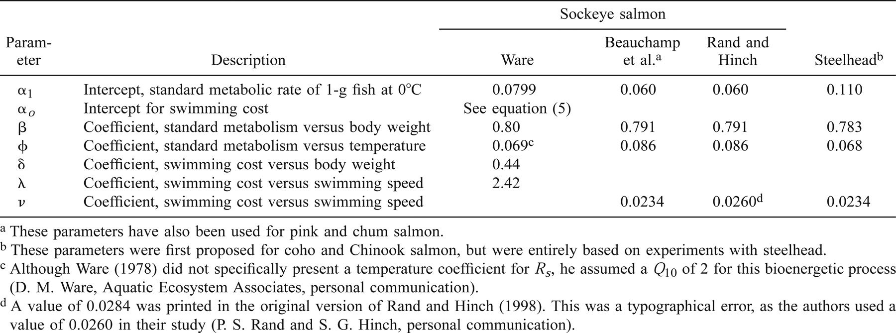

We used equation (4) to estimate αo, and incorporated the empirical values of ρw and μ determined by Miyake and Koizumi (1948) and Dorsey (1968) at various water temperatures (2–24°C) and salinity levels (0–35‰). Substituting ρw and μ by water temperature and salinity, we can estimate αo as

Ware's (1978) model predicts that the oxygen consumption rate of sockeye salmon increases with salinity but decreases with water temperature (Figure 1). These predictions have yet to be tested on sockeye salmon and other species. Ware (1978) then estimated RT of sockeye salmon as the sum of Rs and Ra.
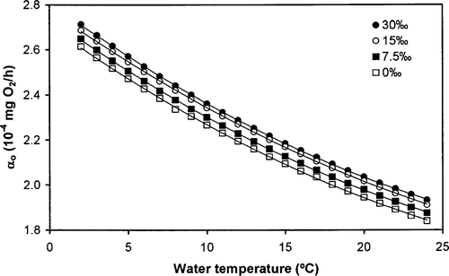
Relationships between the swimming cost coefficient (αo; × 10−4 mg O2/h) derived from Ware (1978) for sockeye salmon and water temperature at four different salinity levels
The second metabolic rate model of sockeye salmon was developed by Beauchamp et al. (1989) as


Pink Salmon and Chum Salmon
Metabolic rates of pink salmon and chum salmon have usually been estimated with the model derived by Beauchamp et al. (1989) for sockeye salmon (Hanson et al. 1997; Davis et al. 1998), probably due to the scarcity of experimental data for pink salmon and the lack of data for chum salmon. Because sockeye salmon, pink salmon, and chum salmon cluster together in phylogenetic analyses based on DNA (McKay et al. 1996), it may seem reasonable to use one model for these species. However, the growth schedules and life histories of these fish are quite different (Groot and Margolis 1991). More importantly, large differences in the metabolic rates of adult sockeye salmon and pink salmon have been reported (Williams and Brett 1987; Brett 1995), suggesting that a single model of respiration rate might not be appropriate for these species.
Coho Salmon, Chinook Salmon, and Steelhead
Stewart and Ibarra (1991) proposed a model based on equation (6) to estimate the metabolic rates of coho salmon and Chinook salmon (Table 1). However, their model was entirely based on the experimental data obtained by Rao (1967) on small steelhead (1–200 g) raised in freshwater. The parameters of this respiration model were later used by Rand et al. (1993) to derive a bioenergetic model for steelhead. It is not known whether this model provides accurate estimates of oxygen consumption rates when it is applied to coho salmon and Chinook salmon.
Freshwater versus Salt Water
Anadromous populations of salmon and trout experience a wide range of salinities throughout their life cycle as they migrate between freshwater and seawater (S = 30–35‰). Thus it might be important to consider the effects of salinity on salmon and trout metabolic rates. None of the models presented in this section, with the exception of Ware's (1978) model, make any explicit statement about the effects of salinity on oxygen consumption of salmon and trout. It has usually been assumed that respiration models derived for salmon maintained in freshwater were also valid in seawater (Brodeur et al. 1992; Davis et al. 1998). However, Rao (1967) and Morgan and Iwama (1991) showed that metabolic rates of steelhead and Chinook salmon were about 30% higher in seawater than in freshwater. In addition, growth efficiency of Arctic char Salvelinus alpinus raised in seawater was lower than that of fish raised in freshwater, also suggesting that salmonid metabolic rates are higher in seawater (Arnesen et al. 1994). Thus, the effects of salinity should be incorporated in models of salmon and trout respiration. As these fish spend only a short time at intermediate salinities during migration between the ocean and streams, it might be sufficient for the purposes of bioenergetic modeling to only assess how the oxygen consumption of salmon and trout varies between freshwater and seawater.
In summary, four models of salmon and trout metabolic rates have been proposed so far: three are more or less specific to sockeye salmon and one is specific to steelhead. The models have been applied to other species within the same genus, usually without verification of the models' validity for other salmonids. Some of these models were developed based on juvenile or small fish (1–200 g) and have been applied to much larger fish (1–5 kg), under the assumption that allometric relationships derived for juvenile fish were valid for larger fish. Finally, except for Ware's (1978) model, the effects of salinity on metabolic rates of salmon and trout has not been considered in bioenergetic models, but may be important given the available experimental evidence.
Methods
Data collection.—We evaluated the four models by comparing Pacific salmon and steelhead metabolic rates extracted from the literature with values predicted by these models. The Rs and RT of Pacific salmon and steelhead were taken directly from tables or extracted from figures by use of a digitizer (Table 2). Whenever possible, we consulted the original source (often a thesis or government report) that was used in these articles to obtain the raw data. The Ra was estimated as the difference between RT and Rs. Fish mass, total length, water temperature, salinity, and swimming speed were noted. When total length was not reported, it was estimated from a length–weight relationship derived for each species. We only used experiments in which fish were forced to swim against a unidirectional current and at a constant swimming speed either in freshwater or in 30 ± 3‰ salt water. Fish swimming at velocities lower than 0.5 body lengths per second were excluded from our analyses, as this velocity is not sufficiently high to keep salmon swimming at a constant speed (Brett 1964). Fish that were reported to show signs of fatigue by the original authors were excluded from our analysis, as an unknown fraction of their swimming metabolism was derived through the anaerobic pathway and was not quantified in these studies. We also excluded experiments in which transmitters or other devices were attached to fish, as the drag and extra load associated with these objects can significantly alter the relationship between swimming cost and swimming speed (Webb 1971).
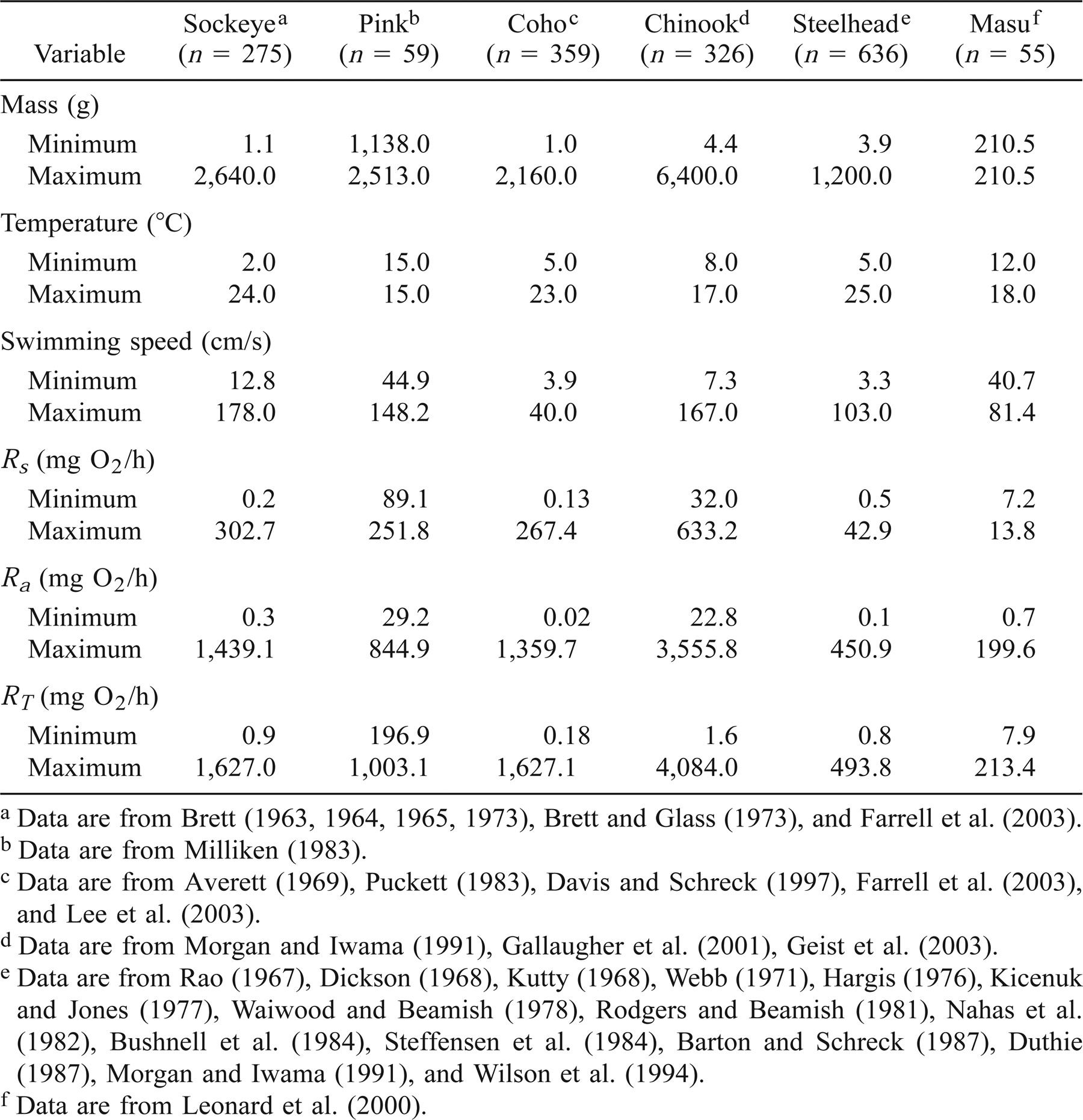
Metabolic rates were extracted from the literature for sockeye salmon, pink salmon, Chinook salmon, coho salmon, and masu salmon raised in freshwater, and for steelhead raised in freshwater and salt water (Table 2). No metabolic rate data were available for chum salmon. The range of fish sizes was narrow for pink salmon and masu salmon, while the range of water temperatures was narrow only for pink salmon (Table 2). A compilation of the data used in this study is available in Trudel and Welch (2002). Additional data were also obtained from Dickson (1968), Kutty (1968), Brett (1973), Hargis (1976), Nahas et al. (1982), Steffensen et al. (1984), Barton and Schreck (1987), Wilson et al. (1994), Davis and Schreck (1997), Morgan and Iwama (1998), Farrell et al. (2003), Geist et al. (2003), and Lee et al. (2003).
Statistical analyses.—Three approaches were used to evaluate the four models. First, the null hypothesis that the slope and intercept of the relationship between predicted and observed values of Rs, Ra, and RT were equal to 1 and 0, respectively, was tested by the ordinary least squares regression method, followed by a chi-square analysis (Jolicoeur 1991) as

where b0 is the estimated intercept, b1 is the estimated slope, Sb0 is the standard error of the intercept, Sb1 is the standard error of the slope, and 0 is the expected intercept and 1 is the expected slope when there are no significant differences between observed and predicted values. The chi-square analysis has two degrees of freedom (Jolicoeur 1991). Second, the degree and source of error in the model predictions were determined by partitioning the mean squared error (MSE) of the relationship between predicted and observed values (Rice and Cochran 1984). The mean component (MC) indicates the bias due to the difference between predicted and observed means. The slope component (SC) indicates the bias resulting from the deviation of the slope from 1. The residual component (RC) indicates the proportion of the overall error that represents random error. The errors of the model are not considered systematic when MC and SC are close to 0 and when RC is close to 1. Third, the reliability index (Ks) of Leggett and Williams (1981) was also calculated. This reliability index indicates that approximately 68% of the observed values are within a factor of Ks of the predicted values. The closer Ks is to 1, the better the fit between predicted and observed values. These analyses were performed on natural log-transformed data to homogenize the variance (Sokal and Rohlf 1995). The three procedures outlined above evaluate the accuracy, bias, and precision of the model.
Extrapolation of respiration models between life stages.—To determine whether allometric equations of metabolic rates could be extrapolated to different life stages or size-classes, we developed models of Rs, Ra, and RT independently for small (1–130 g) and large (690–2,200 g) sockeye salmon with the experimental data extracted from Brett (1963, 1964, 1965) and Brett and Glass (1973). These size ranges were used to separate small and large fish, as there was a gap in the size distribution between 130 and 690 g in our data. Multiple regression analyses were used to assess the effects of water temperature, mass, and swimming speed on Rs, Ra, and RT. Except for water temperature, all the variables were natural log-transformed prior to the analyses to linearize the relationships and homogenize the variances (Sokal and Rohlf 1995). Variables that were not significant at the 0.05 level were dropped from the regression models. The RT was also estimated as the sum of Rs and Ra by use of the regression equations derived for Rs and Ra. We then used the models developed for small sockeye salmon to predict Rs, Ra, and RT of large sockeye salmon. Conversely, we also used the models developed for large sockeye salmon to predict Rs, Ra, and RT of small sockeye salmon. Predicted and observed values were then compared by use of the three evaluation procedures outlined above.
Growth of sockeye salmon.—The importance of biases in model parameters depends largely on the application and on the precision desired by the user. Sensitivity analyses have generally shown that a 10% error in metabolic costs can produce an error greater than 10% in bioenergetic model output (Kitchell et al. 1977; Stewart et al. 1983). However, biases associated with the metabolic rates of Pacific salmon and steelhead can range from 0% to 250% depending on fish size and water temperature (see Results).
To assess the effects of these biases, we fitted a bioenergetic model to the mean weight of sockeye salmon caught during various months in offshore waters of the North Pacific Ocean, as reported by Ishida et al. (1998). We then modified Rs and Ra by ±10%, ±30%, and ±50% to simulate typical biases observed in this study and examined the effect of these biases on the growth trajectory of sockeye salmon during their marine life. For these simulations, we estimated Rs as

and Ra as

These parameters were obtained by reanalyzing the sockeye salmon oxygen consumption data used in this study (M. Trudel, unpublished). We assumed that Rs of sockeye salmon was 28% higher in seawater (Rao 1968). We used an energy equivalent of 3.24 cal/mg O2 to convert oxygen consumption into energy units (Elliott and Davison 1975).
From equations (9) and (10), we derived the following optimal cruising speed (Uc.opt; cm/s) for estimating the swimming speed of sockeye salmon at sea (M. Trudel, unpublished):

For simplicity, we assumed that waste production and specific dynamic action represented a total of 40% of the fish's energy budget. We also assumed that the prey energy density was 1,000 cal/g (wet weight). This value is well within the range of published energy densities of sockeye salmon prey in the North Pacific Ocean (Davis et al. 1998). Temperature was modeled based on the temperature cycle provided in Brett (1983). We assumed that sockeye salmon smolts entered the ocean on May 15 at 5 g and spent 3 years in the ocean.
Results
Model Evaluation
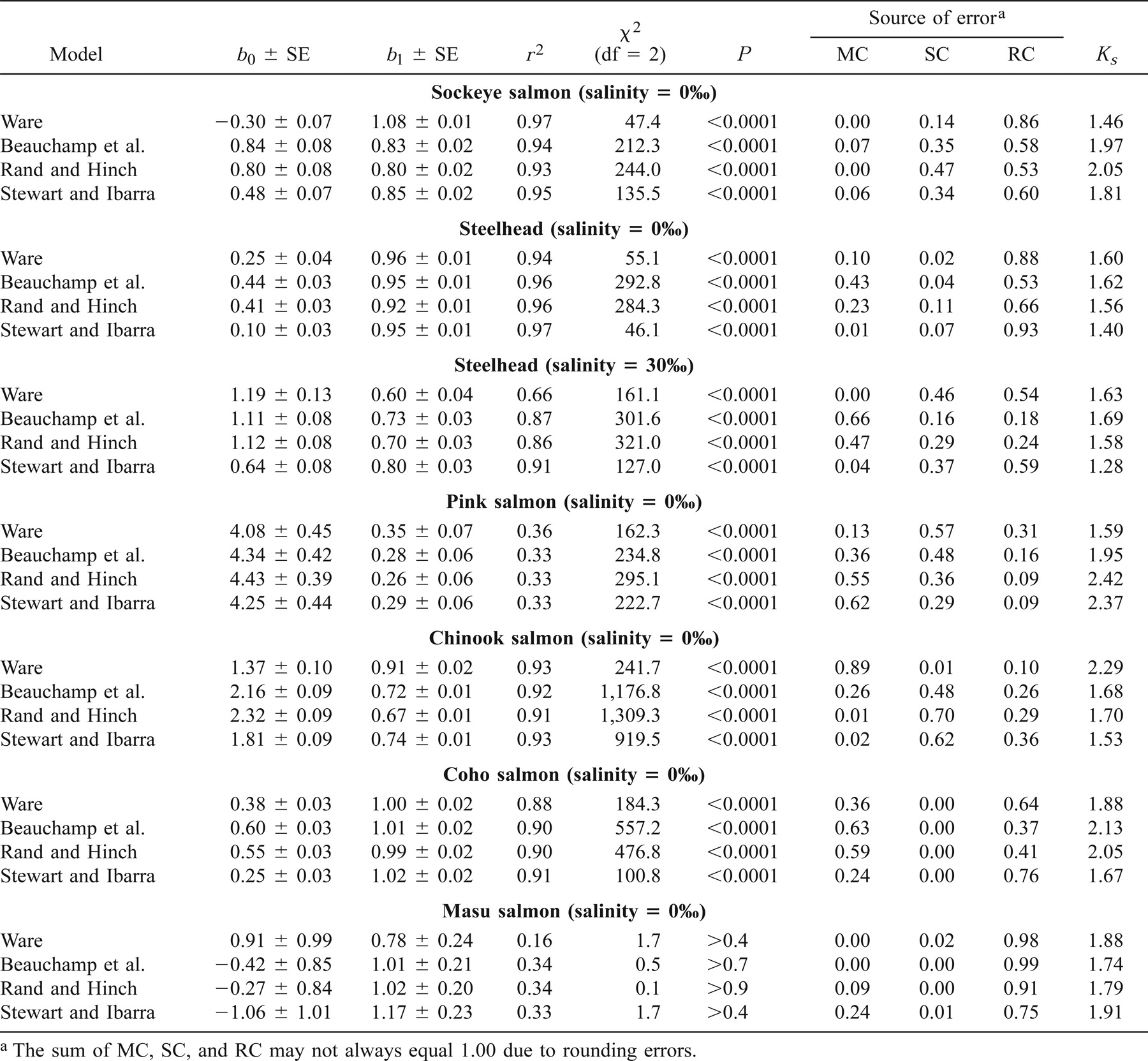
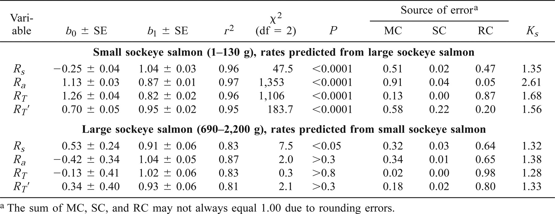
The Rs of sockeye salmon was predicted fairly well by the Ware (1978) model, the Beauchamp et al. (1989) model, and the Rand and Hinch (1998) model (Figure 2; note that these are log–log plots). Although the relationship between predicted and observed Rs tended to differ significantly from the 1:1 line (Table 3), the systematic biases introduced by these models were low for most combinations of water temperature and fish size (Figure 2). For instance, Ware's (1978) model overestimated Rs of sockeye salmon kept in cold water by about 15–30%, while the Beauchamp et al. (1989) model and the Rand and Hinch (1998) model underestimated the Rs of small sockeye salmon kept in warm water and overestimated the Rs of large sockeye salmon kept in cold water by about 25–35% (Figure 2). The Ks ranged between 1.33 and 1.37 for sockeye salmon (Table 3), indicating that predicted values were usually within 33–37% of the observed values.
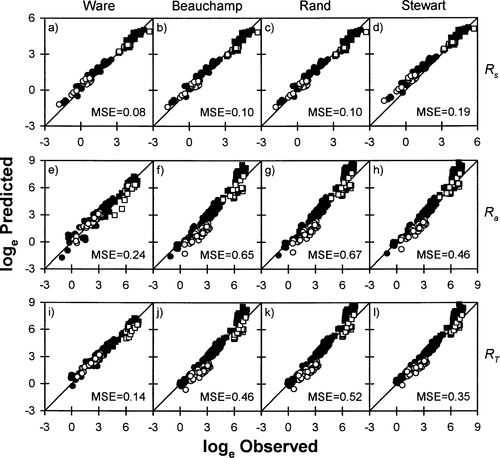
Relationships between observed and predicted (A–D) standard metabolic rates (Rs; mg O2/h), (E–H) swimming costs (Ra; mg O2/h), and (I–L) total metabolic costs (RT; mg O2/h) of sockeye salmon in freshwater, based on four models (Ware 1978; Beauchamp et al. 1989; Stewart and Ibarra 1991; Rand and Hinch 1998). The solid diagonal line represents 1:1 correspondence between the variables. Values above the line overestimate metabolic rates, while values below the line underestimate metabolic rates. Open symbols represent cold water temperatures (2–12°C); closed symbols represent warm water temperatures (14–24°C). Circles denote small fish (1–300 g), and squares denote large fish (690–2,230 g). Mean squared error (MSE) is shown for each relationship. Note that there is a different scale for each panel

In general, Ra of sockeye salmon was adequately predicted by Ware's (1978) model (Figure 2; Table 4). The average bias ranged from 8% to 25%, depending on fish size and water temperature (Figure 2). The Beauchamp et al. (1989) model and the Rand and Hinch (1998) model did not accurately predict Ra of sockeye salmon for most combinations of water temperature and size (Figure 2; Table 4). Both models systematically underestimated Ra of small sockeye salmon by a factor of 1.3–3.3, and overestimated Ra in large sockeye salmon kept in warm water by a factor of 2.4–3.6 (Figure 2). The Ks was also quite large (i.e., >2) for these two models (Table 4). The relationship between observed and predicted Ra differed significantly from the 1:1 line for both models (Table 4).

The predictions obtained for RT in sockeye salmon mirrored those obtained for Ra (Figure 2). Large systematic biases were obtained with the Beauchamp et al. (1989) model and the Rand and Hinch (1998) model, while the Ware (1978) model performed fairly well for most combinations of water temperature and fish size (Figure 2; Table 5).
The Rs values of steelhead raised in freshwater were, with the exception of a cluster of points extracted from Wilson et al. (1994), accurately predicted by Stewart and Ibarra's (1991) model, as indicated by the low dispersion of the points around the 1:1 line (Figure 3). The values from Wilson et al. (1994) were overestimated by a factor of 2.5 (Figure 3). The bias for Rs extracted from the nine other studies ranged from 0% to 35%. The Stewart and Ibarra (1991) model also accurately predicted Ra and RT for steelhead raised in freshwater, although Ks was large for Ra (Figure 3; Tables 4, 5). In particular, the model tended to underestimate Ra of small steelhead held in cold freshwater by about 32% (Figure 3). Although Stewart and Ibarra's (1991) model was derived from small fish (30–150 g), this model accurately predicted the oxygen consumption of larger steelhead (300–1,200 g).
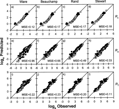
Relationships between observed and predicted (A–D) standard metabolic rates (Rs; mg O2/h), (E–H) swimming costs (Ra; mg O2/h), and (I–L) total metabolic cost (RT; mg O2/h) of steelhead in freshwater, based on four models (Ware 1978; Beauchamp et al. 1989; Stewart and Ibarra 1991; Rand and Hinch 1998). See Figure 2 for explanation of symbols.
Stewart and Ibarra's (1991) model tended to systematically underestimate Rs of steelhead raised in seawater by about 15–25% (Figure 4). The relationship between observed and predicted Rs also differed significantly from the 1:1 line for these fish (Table 3). The model also slightly overestimated Ra of steelhead raised in warm seawater (Figure 4). As a result, this model tended to underestimate RT of steelhead maintained in cold seawater and overestimate RT of steelhead kept in warm seawater (Figure 4), though these biases were quite small (<20%; Table 5). Overall, however, the Rs, Ra, and RT predicted for steelhead by Stewart and Ibarra's (1991) model were usually quite close to observed values in both freshwater and seawater.
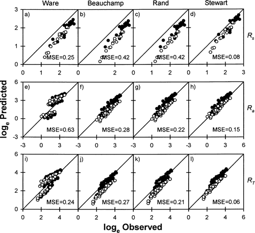
Relationships between observed and predicted (A–D) standard metabolic rates (Rs; mg O2/h), (E–H) swimming costs (Ra; mg O2/h), and (I–L) total metabolic costs (RT; mg O2/h) of steelhead in salt water, based on four models (Ware 1978; Beauchamp et al. 1989; Stewart and Ibarra 1991; Rand and Hinch 1998). See Figure 2 for explanation of symbols
Extrapolation of Respiration Models between Species
The sockeye salmon models (Ware 1978; Beauchamp et al. 1989; Rand and Hinch 1998) tended to underestimate the Rs of steelhead, pink salmon, and Chinook salmon (Figures 3–5, 7; Table 3), the Ra of coho salmon, Chinook salmon, and masu salmon (Figures 6–8; Table 4), and the RT of steelhead, coho salmon, Chinook salmon, and masu salmon (Figures 3, 4, 6–8; Table 5). The average bias produced by these models ranged from 0% to 250% (Figures 3–8). In addition, the observed Rs and RT of pink salmon were poorly correlated with the predictions obtained from the sockeye salmon models (Figure 5; Tables 4, 5). The Ks was particularly high for the Rs, Ra, and RT of pink salmon predicted with the sockeye salmon models (Tables 3–5).

Relationships between observed and predicted (A–D) standard metabolic rates (Rs; mg O2/h), (E–H) swimming costs (Ra; mg O2/h), and (I–L) total metabolic costs (RT; mg O2/h) of pink salmon in freshwater, based on four models (Ware 1978; Beauchamp et al. 1989; Stewart and Ibarra 1991; Rand and Hinch 1998). See Figure 2 for explanation of symbols
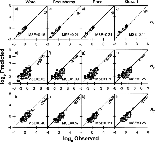
Relationships between observed and predicted (A–D) standard metabolic rates (Rs; mg O2/h), (E–H) swimming costs (Ra; mg O2/h), and (I–L) total metabolic costs (RT; mg O2/h) of Chinook salmon in freshwater, based on four models (Ware 1978; Beauchamp et al. 1989; Stewart and Ibarra 1991; Rand and Hinch 1998). See Figure 2 for explanation of symbols

Relationships between observed and predicted (A–D) standard metabolic rates (Rs; mg O2/h), (E–H) swimming costs (Ra; mg O2/h), and (I–L) total metabolic costs (RT; mg O2/h) of coho salmon in freshwater, based on four models (Ware 1978; Beauchamp et al. 1989; Stewart and Ibarra 1991; Rand and Hinch 1998). See Figure 2 for explanation of symbols
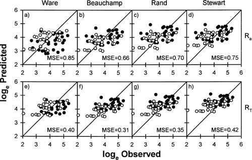
Relationships between observed and predicted (A–D) swimming costs (Ra; mg O2/h) and (E–H) total metabolic costs (RT; mg O2/h) of masu salmon in freshwater, based on four models (Ware 1978; Beauchamp et al. 1989; Stewart and Ibarra 1991; Rand and Hinch 1998). See Figure 2 for explanation of symbols
The steelhead model (Stewart and Ibarra 1991) tended to underestimate Rs and overestimate Ra and RT of pink salmon (Figure 5; Tables 3–5). The model overestimated the Rs of sockeye salmon and coho salmon (Figures 2, 6; Table 3), but underestimated the Ra and RT of coho salmon and masu salmon (Figures 6, 8; Tables 4, 5). For Chinook salmon, the steelhead model underestimated Ra and RT at the lower ranges of these values and overestimated Ra and RT at the higher ranges (Figure 7). Stewart and Ibarra's (1991) steelhead model outperformed the Beauchamp et al. (1989) model and the Rand and Hinch (1998) model for predicting Ra and RT of sockeye salmon (Figure 2; Tables 4, 5). Nevertheless, Stewart and Ibarra's (1991) steelhead model also produced large systematic biases for small sockeye salmon maintained in cold water and large sockeye salmon maintained in warm water (Figure 2). The steelhead model also produced fairly large values of Ks for the Ra and RT of sockeye salmon, pink salmon, coho salmon, and masu salmon (Tables 4, 5), indicating that predicted values were quite far from observed values. On average, the bias produced by Stewart and Ibarra's (1991) steelhead model ranged from about 5% to 250% when applied to sockeye salmon, pink salmon, Chinook salmon, coho salmon, and masu salmon (Figures 2–8).
Overall, biases associated with metabolic rates ranged from close to 0% to over 200%, depending on fish size and water temperature, with about two-thirds of these values exceeding 20% (Figure 9). The median and average biases were 33% and 42%, respectively (Figure 9).
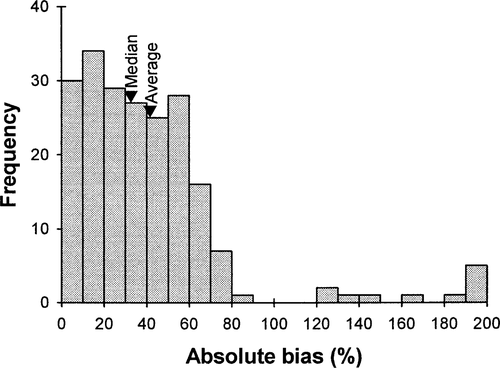
Frequency distribution of biases associated with the predictions of four oxygen consumption rate models (Ware 1978; Beauchamp et al. 1989; Stewart and Ibarra 1991; Rand and Hinch 1998). Biases were averaged for a given combination of fish size (small versus large), temperature (cold versus warm), species, and model
Extrapolation of Respiration Models between Life Stages
Fish mass, water temperature, and swimming speed explained 84–98% of the variance associated with Rs, Ra, and RT of small and large sockeye salmon (Table 6). Except for RT, the same variables were retained in the regression models used to predict the metabolic rates of both small and large sockeye salmon (Table 6). Swimming cost was not significantly correlated to water temperature in either small sockeye salmon (F1,99 = 2.6; P > 0.1) or large sockeye salmon (F1,55 = 3.2; P > 0.05). Although the values of the regression coefficients varied somewhat between small and large sockeye salmon, the confidence intervals of these coefficients overlapped (Table 6), indicating that the regression equations were similar for the two life stages.

The metabolic rate models derived from large sockeye salmon systematically overestimated Rs and underestimated Ra and RT of small sockeye salmon (Table 7; Figure 10). Interestingly, the bias of RT was smaller when it was estimated as the sum of Rs and Ra than when it was directly derived from a single regression equation (Table 7; Figure 10E, G). In contrast, the juvenile model accurately predicted the metabolic rates of large sockeye salmon (Table 7; Figure 10). Except for Rs, the relationship between observed and predicted values did not deviate significantly from the 1:1 line (Table 7; Figure 10). However, the juvenile model tended to overestimate Ra of large sockeye salmon maintained in warm water by about 35% (Figure 10).

Relationships between observed and predicted (A, B) standard metabolic rates (Rs; mg O2/h), (C, D) swimming costs (Ra; mg O2/h), and (E–H) total metabolic costs (RT; mg O2/h) of sockeye salmon. The left panels show metabolic costs of small sockeye salmon (1–130 g) predicted with models derived from adult fish. The right panels show metabolic costs of large sockeye salmon (690–2,200 g) predicted with models derived from juvenile fish. The RT values were estimated either directly from an empirical model (E, F) or as the sum of Rs and Ra(G, H). See Figure 2 for explanation of symbols
Growth of Sockeye Salmon
A reasonable growth trajectory was achieved when sockeye salmon were assumed to be feeding at 68% of their maximum capacity (Cmax) during their first 20 months in the ocean, and at 85% of Cmax thereafter. The sensitivity analyses showed that the bioenergetic model of sockeye salmon was more sensitive to errors associated with Ra than errors associated with Rs (Figure 11). A 30% error in Ra, which was commonly observed in this study, could result in a 35–50% error in the final size of returning adults (Figure 11).
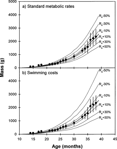
Impact of errors (±10%, ±30%, and ±50%) in standard metabolic rate (Rs) and swimming cost (Ra) on the estimated lifetime growth of sockeye salmon in the ocean. The error bars represent ±1 SD
Discussion
The analyses performed in this study showed that (1) oxygen consumption rates for sockeye salmon and steelhead were not always accurately predicted by models that were derived specifically for these species, (2) metabolic rates of Pacific salmon and steelhead were not accurately predicted by models derived from closely related species, and (3) allometric equations of metabolic rates were not stable when measured over small ranges of sizes, and were inaccurate when extrapolated to smaller or larger fish. These results imply that serious biases could be introduced by the use of these models. In addition, our results indicate that models should be carefully built to avoid introducing biases. Furthermore, the impact of the biases should be evaluated to determine whether or not the interpretations associated with the use of these models are seriously affected.
Model Evaluation
In fish, estimates of oxygen consumption rate have been mostly used with bioenergetic models for estimating food consumption rates or predicting growth rates. Models of oxygen consumption rates have generally been considered accurate and reliable when bioenergetic model predictions agreed with independent estimates of food consumption or growth rates (Rice and Cochran 1984; Beauchamp et al. 1989; Madenjian and O'Connor 1999). However, a close correspondence between independent estimates should not be taken as evidence that the parameters of the model are accurate and valid, since this can occur even if the two estimates are erroneous (Ney 1993). Model validation should be assessed by comparing model predictions with direct measurements. In this study, we directly determined the accuracy of published models of oxygen consumption rates of sockeye salmon and steelhead by contrasting model predictions with oxygen consumption rates measured under controlled conditions of size, water temperature, swimming speed, and salinity. Our analyses showed that, in general, oxygen consumption rates of steelhead were adequately predicted by the model proposed by Stewart and Ibarra (1991) for sizes between 4 and 1,200 g. However, their model performed poorly on standard metabolic rates derived by Wilson et al. (1994): these values were overestimated by a factor of three. It is unclear why this occurred, as the standard metabolic rates that were extracted from nine other studies were accurately predicted by Stewart and Ibarra's (1991) model.
Our analyses showed that oxygen consumption rates of sockeye salmon tended to be accurately predicted by Ware's (1978) model, but not by the Beauchamp et al. (1989) and Rand and Hinch (1998) models. In particular, the latter two models underestimated RT of small sockeye salmon in cold water by 50–60% and overestimated RT of large sockeye salmon in warm water by 130–230%. Our analyses also indicated that the adjustments made by Rand and Hinch (1998) reduced the performance of the original model proposed by Beauchamp et al. (1989). Therefore, the validity of the conclusions reached by studies that used either the Beauchamp et al. (1989) model or the Rand and Hinch (1998) model may need to be reassessed.
The model derived by Beauchamp et al. (1989) is one of the few bioenergetic models that have been successfully corroborated against independent estimates. The authors showed that cumulative consumption rates predicted with their bioenergetic model were within 10% of those obtained from stomach contents for Lake Washington juvenile sockeye salmon. However, the model was tested on small sockeye salmon (0.1–15 g) inhabiting cold water (6–10°C). The analyses performed in our study indicated that, under these conditions of size and temperature, the Beauchamp et al. (1989) model likely underestimated oxygen consumption rates of sockeye salmon by about 50%, which suggests that their bioenergetic model also underestimated food consumption rates. To evaluate the effect of this bias on their model predictions, we estimated food consumption rates of Lake Washington sockeye salmon from their bioenergetic model, and we used equations (9) and (10) to estimate oxygen consumption rates. Our analyses showed that the bioenergetic model of Beauchamp et al. (1989) underestimated food consumption rates by 26%. Hence, the close correspondence between fish stomach contents and the food consumption rates derived with their bioenergetic model may have been coincidental.
Rand and Hinch (1998) also successfully tested their bioenergetic model with independent estimates. The authors demonstrated that their model adequately described the energy depletion of adult Fraser River sockeye salmon during upriver migration. However, the model was tested on large sockeye salmon (2.88 kg) inhabiting warm water (15–21°C). To determine the magnitude of the bias in their study, we compared the energy depletion of sockeye salmon during upriver migration based on Rand and Hinch's (1998) oxygen consumption model and based on equations (9) and (10). Initial fish size, energy density, and fat content were set to 2.88 kg, 8,370 J/g, and 15%, respectively (Rand and Hinch 1998). Swimming speed was set to 75 cm/s, which is within the range of values observed by Hinch and Rand (1998) for Fraser River sockeye salmon during upriver migration. We assumed that sockeye salmon utilized only lipids during migration, and estimated weight loss based on the assumption that the energy density of fat was 39.5 kJ/g (Brett 1973). Hence, we assumed that sockeye salmon lost 1 g for each 39.5 kJ of energy utilized during migration. We further assumed that water temperature was 15°C and that migration was completed in 24 d (Rand and Hinch 1998). The Rand and Hinch (1998) model overestimated oxygen consumption rates of sockeye salmon by 27%, but overestimated energy depletion by only 6.6% over the 24-d period. Thus, the bias produced by their model was small at the 75-cm/s swimming speed. However, the magnitude of the bias increased with water temperature and swimming speed. For instance, at 20°C, the model overestimated energy depletion by 46% for sockeye salmon swimming at 95 cm/s. In addition, the model predicted that lipid content dropped to 1.9% after 24 d, compared to 9.5% for equations (9) and (10). Thus, the Rand and Hinch (1998) model should be applied carefully, as it may not be appropriate for every situation.
Models based on experiments performed in swimming tunnels are likely to be inaccurate for estimating the energetic costs of fish in the wild. In swimming tunnels, fish are typically forced to swim against a unidirectional current at a constant speed. In contrast, fish must frequently change direction and speed in a turbulent environment such as a river or stream. Empirical and laboratory studies have shown that oxygen consumption rates increase with swimming complexity, possibly due to the cost of accelerating and changing direction (Boisclair and Tang 1993; Krohn and Boisclair 1994; Tang and Boisclair 1995). Hence, the model of Rand and Hinch (1998) would be expected to underestimate swimming costs of salmon in rivers and streams. Swimming tunnels may still be appropriate for pelagic fishes, as swimming complexity tends to be lower in open habitats (Tang and Boisclair 1993).
Bioenergetic models are more frequently used to estimate food consumption rates than to predict growth rates, as growth rates tend to be more sensitive to parameter uncertainty, possibly because the error is compounded over time (Kitchell et al. 1977; Stewart et al. 1983; Hanson et al. 1997). The simulations performed in our study also showed that growth predicted with bioenergetic models was sensitive to errors associated with metabolic rates: a 30% error in Rs produced a 680-g error in the lifetime growth of sockeye salmon, and a 30% error in Ra produced a 1.1-kg error in lifetime growth. Thus, the impact of the biases observed in our study will largely depend on the application of the models. Our work further indicates that the effects of biases on model predictions should be evaluated based on a large range of values.
It is important to note that the models we tested performed reasonably well (bias < 15%) under certain conditions of fish size and water temperature. For instance, the average bias associated with the Beauchamp et al. (1989) and Rand and Hinch (1998) models was around 5–10% for Rs of small sockeye salmon in cold water and large sockeye salmon in warm water, and for Ra and RT of small sockeye salmon in warm water. Thus, under these conditions, the two models could be applied without seriously affecting the accuracy of bioenergetic models.
Influence of Salinity on Oxygen Consumption Rates
The analyses performed in this study indicated that the model of Stewart and Ibarra (1991) systematically underestimated Rs of steelhead in salt water by 15–25%. In addition, Ra was slightly overestimated by their model. Hence, due to the systematic biases in the predictions of Rs and Ra, their model may not be appropriate for estimating the individual components of the metabolism of steelhead in seawater. A possible explanation is that osmoregulation costs are higher in seawater than in freshwater due to increased gill Na+,K+-ATPase activity in salt water (Morgan and Iwama 1991; Maxime 2002). Changes in hormonal activity (Morgan and Iwama 1991) and ventilatory activity (Maxime 2002) following transfer to seawater may also be involved. In contrast to our study, Morgan and Iwama (1998) showed that oxygen consumption rates of juvenile coho salmon acclimated to freshwater, isosmotic water, and seawater (28‰) were not significantly different. They suggested that the effects of salinity on oxygen consumption rates of salmonids may be influenced by developmental stage (e.g., fry versus juvenile) and life history (e.g., landlocked versus anadromous). Further work will be required to understand and quantify the effects of salinity on salmonid metabolic rates.
Extrapolation of Respiration Models between Species
Bioenergetic models require the estimation of a large number of parameters. Due to the scarcity of empirical and experimental data, it has often been necessary to borrow these parameters from other species or extrapolate them to other life stages or sizes. The analyses we performed showed that metabolic rates varied significantly among species of the genus Oncorhynchus. In addition, we found that, in general, models derived from closely related species did not accurately predict salmonid metabolic rates. This suggests that the practice of “species borrowing” should be avoided, at least for metabolic rates, as large biases are likely to be introduced when metabolic rate models are extrapolated to other species. However, this does not imply that general models based on the compilation of data obtained from a large number of species are futile, as the necessity of using species-specific parameters for metabolic rates of fish will depend primarily on the sensitivity of the studied process to metabolic rates and on the precision required by the investigators.
Metabolic rates of pink salmon and chum salmon have usually been determined from the model derived by Beauchamp et al. (1989) for sockeye salmon (e.g., Hanson et al. 1997; Davis et al. 1998), while those of coho salmon and Chinook salmon have been estimated from Stewart and Ibarra's (1991) model (e.g., Stewart et al. 1991; Brodeur et al. 1992; Rand and Stewart 1998). Our analyses showed that the metabolic rates of pink salmon, Chinook salmon, coho salmon, and masu salmon were not accurately estimated with these two models. However, it is important to note that the scope of our evaluation is limited to 1–2,160-g coho salmon, 210-g masu salmon, 1.2–2.5-kg pink salmon, and 4.4–6,400-g Chinook salmon. At this point, it is not possible to determine whether the models we evaluated can accurately predict the oxygen consumption rates of other size-classes of these species.
Extrapolation of Respiration Models between Life Stages
The analyses we performed suggest that metabolic rates of adult sockeye salmon can be adequately estimated from a model derived from juvenile sockeye salmon. Similar results were obtained for steelhead, as Stewart and Ibarra's (1991) model accurately predicted the metabolic rates of large steelhead in freshwater even though it was derived from small fish. This suggests that metabolic rate models developed based on juvenile fish may be extrapolated to larger and potentially mature fish. However, this practice should be carefully evaluated before it is broadly applied. In addition, our analyses showed that the metabolic rates of juvenile sockeye salmon were not accurately predicted with models derived from adult fish. These differences may be attributed to the range of sizes used to construct these metabolic rate models. While the absolute size range was larger for the adult model than the juvenile model (1,510 g versus 129 g), the relative size range was much greater for the juvenile model than the adult model (130-fold versus threefold). This suggests that the allometric exponent of salmon respiration is less stable when it is estimated over a small range of sizes, and that metabolic rate models based on a size range that covers at least two orders of magnitude may be extrapolated between life stages (except for early life history) without seriously biasing the predictions. Similar results have been obtained by Dodds et al. (2001) for birds and mammals. However, additional studies will be necessary before these results can be generalized to other species.
Implications for Bioenergetic Modeling
Bioenergetic models are particularly sensitive to errors associated with metabolic rates (Kitchell et al. 1977; Stewart et al. 1983). Our analyses showed that the biases introduced by estimating the metabolic rates from another closely related species were usually much greater than 10%, indicating that accurate estimates of metabolic rates are needed for field applications, and that bioenergetic models may not always be appropriate for providing absolute estimates of growth or consumption rates. Despite the economic and cultural importance of salmonids, little is known about the metabolic rates of most salmon species. For instance, we were unable to find any published estimates of metabolic rate for chum salmon. The experiments performed on coho salmon, Chinook salmon, pink salmon, and masu salmon covered only a limited range of sizes and/or water temperatures (e.g., Averett 1969; Milliken 1983; Puckett 1983; Leonard et al. 2000). Thus, if we were to construct metabolic rate models for these species with the limited data that are currently available, it would be necessary to extrapolate them well beyond the ranges of size and water temperature available from experimental observations. Moreover, although salmon spend the majority of their life cycle in the ocean, the effects of salinity on their metabolic rates has rarely been examined and is poorly understood. Further studies are clearly necessary to measure the metabolic rates of more Pacific salmon species under a wider range of conditions. As body size explains most of the variability in Rs and Ra, it might be more appropriate to perform these experiments on a few fish that cover a large range of sizes than on many fish covering a narrow range of sizes.
It may be argued that, despite the biases observed in this study, bioenergetic models could still be used to compare estimates on a relative basis or to contrast the outcome of various scenarios. This approach could provide meaningful insights as long as the magnitude and direction of the biases are consistent across comparisons. However, given that the biases observed in this study were not always consistent across size-classes and temperatures, it may be difficult to properly interpret differences in model predictions for different size-classes or thermal regimes. For instance, the bioenergetic model of Stewart and Ibarra (1991) overestimated saltwater oxygen consumption rates of steelhead at cold temperatures and underestimated oxygen consumption at warm temperatures. Thus, it might not be possible to separate the effects of temperature versus model bias in salt water. In addition, comparisons of model predictions should be limited to the same species, as differences obtained among species may be due to species-specific effects or to uncertainty in the parameters. For instance, Standen et al. (2002) recently estimated the energetic costs of migration in Fraser River pink salmon and sockeye salmon. Their analyses showed that energy expenditures were similar for both species during migration. However, these results may have been obtained because the authors used the model of Rand and Hinch (1998) to estimate the oxygen consumption rates of both species. Our analyses indicated that the Rand and Hinch (1998) model overestimated oxygen consumption rates of pink salmon by 100–150% for fish swimming at the average speed observed by Standen et al. (2002). Thus, unrecognized differences among species could lead to incorrect conclusions.
Bioenergetic models also require a conversion factor to transform oxygen consumption rates to energy units. This has usually been achieved by use of an oxycalorific equivalent of 3.24 cal/mg O2 (Elliott and Davison 1975). This approach assumes that the contribution of anaerobic metabolism is negligible during swimming. While this may be a reasonable assumption at slow-to-moderate swimming speeds, it may not be valid when swimming speed approaches the maximum sustainable speed (Ucrit). Wilson and Egginton (1994) showed that anaerobic power was recruited at 94% of Ucrit in steelhead. In contrast, Burgetz et al. (1998) showed that anaerobic metabolism occurred at 70% of Ucrit for the same species. Clearly, more work is necessary to assess the importance of anaerobic metabolic rates, and to incorporate these costs into bioenergetic models. In addition, accurate empirical models of Ucrit will be necessary to determine the appropriate situations for adding the bioenergetic costs of anaerobic power.
There is an increasing demand for complex biophysical models to understand the functioning of ecosystems by integrating trophic interactions, bioenergetics, and the physical structure of the environment. The accuracy of the predictions achieved with such models depends largely on our ability to adequately estimate the various components that are incorporated into the models. The number of parameters to estimate in these models quickly increases with the number of processes and interactions that are modeled. Unfortunately, the data required for estimation of these parameters are often not available, even in well-studied species like Pacific salmon. Hence, increased funding and scientific recognition for basic organismal research will be critical if more realistic ecosystem models are to be achieved.
Acknowledgments
We thank J. E. Zamon, P. S. Rand, S. G. Hinch, and D. J. Randall for useful comments on earlier versions of the manuscript. Financial support was provided by Fisheries and Oceans Canada, the Bonneville Power Administration, and the World Wildlife Fund. M. Trudel was also supported by a Visiting Fellowship in a Canadian Government Laboratory and by a postdoctoral fellowship from the Fonds pour la Formation de Chercheurs et l'Aide à la Recherche.


