Optimization of Sample Size, Data Points, and Data Augmentation Stride in Vibration Signal Analysis for Deep Learning-Based Fault Diagnosis of Rotating Machines
Abstract
In recent years, deep learning models have increasingly been employed for fault diagnosis in rotating machines, with remarkable results. However, the accuracy and reliability of these models in fault diagnosis tasks can be significantly influenced by critical input parameters, such as the sample size, the number of data points within each sample, and the augmentation stride in vibration signal analysis. To address this challenge, this paper proposes a new adaptive method based on Bayesian optimization to determine the optimal combination of these input parameters from raw vibration signals and enhance the diagnostic performance of deep learning models. This study utilizes a one-dimensional convolutional neural network (1-D CNN) as the deep learning model for fault classification. The proposed adaptive 1-D CNN-based fault diagnosis method is validated via vibration signals collected from motor rolling bearings and achieves a fault diagnosis accuracy of 100%. Compared with existing CNN-based diagnosis methods, this adaptive approach not only achieves the highest accuracy on the testing set but also demonstrates stable performance during training, even under varying operating conditions. These results indicate the importance of optimizing the input parameters of deep learning models employed in fault diagnosis tasks.
1. Introduction
Rotating machines are essential and widely used components in various industries, such as manufacturing, power generation, aerospace, and automotive sectors. Common examples of these machines are motors, turbines, generators, engines, and others. Due to the inherent relative motion among essential components—such as bearings, gears, rotors, and shafts—rotating machines are prone to mechanical failures, which can significantly impact the performance of industrial systems [1, 2]. Consequently, diagnosing these faults is crucial to prevent unexpected breakdowns, reduce maintenance costs, and ensure the longevity and reliability of these systems.
Fault diagnosis is the process of detecting, locating, and identifying faults within a system. In recent decades, artificial intelligence has advanced rapidly and has been extensively applied in this field. However, previous studies predominantly focused on traditional intelligent fault diagnosis methods that rely on historical data [3, 4]. These methods often depend on manual analysis and expert knowledge, which can be time-consuming and subjective [5]. Recent advancements in artificial intelligence have led to the increased application of deep learning models in the fault diagnosis of rotating machines. Deep learning models, such as convolutional neural networks (CNNs) [6], recurrent neural networks [7], long short-term memory [8], and generative adversarial networks [9], possess remarkable capabilities for automatically processing and analyzing complex data patterns from raw input signals. This makes these deep learning models well suited for diagnosing faults in rotating machinery.
Among the various input signals utilized for fault diagnosis, vibration signals are especially valuable. These signals provide valuable insights into operating conditions and potential faults [10]. Moreover, vibration signals are highly sensitive to a range of fault types and severities. The characteristics of these signals effectively reflect the real-time condition of the machinery. Despite the advantages of using vibration signals, obtaining a sufficient number of vibration signal samples from operational rotating machines can be challenging. Increasing the sample size has been shown to enhance the generalization ability of deep learning models in fault diagnosis, yet practical limitations exist. This is due to factors, such as the limitations of measuring devices and the complex working conditions under which these machines operate. In addition, certain operational constraints, such as limited access to machines and the need to avoid production interruptions, further restrict the availability of vibration signal samples. It is important to note that deep learning models trained on inadequate samples are susceptible to overfitting, where the model becomes overly specialized to the available data and performs poorly on unseen instances. This raises a crucial question: What is the minimum number of samples required for training deep learning models using vibration signals in the fault diagnosis of rotating machines?
In addition to determining the minimum sample size, establishing the optimal number of data points within each sample is essential in deep learning-based fault diagnosis, particularly when working with raw vibration signals in the time-based form. This parameter, which defines the length of each sample, has a significant impact on the accuracy and effectiveness of fault diagnosis. Typically, researchers select data point sizes that are powers of 2, such as 1024, 2048, or 4096, to ensure compatibility with computational algorithms. In some studies [10, 11], a sample size of 1024 data points was utilized. Other research efforts have opted for 2048 data points per sample [12, 13]. Some other studies have employed an even larger sample size of 4096 data points [14, 15]. Miettinen et al. [16] went further and utilized 8192 data points as the input for analysis in fault diagnosis of drive train gears. The rationale for adopting power-of-2 data point sizes in fault diagnosis applications arises from the compatibility of these sizes with the fast Fourier transform algorithm, which facilitates straightforward and faster calculations due to the binary representation used by computers. This compatibility makes power-of-2 data point sizes advantageous for fault diagnosis, as they facilitate efficient analysis via techniques such as the fast Fourier transform algorithm. Furthermore, studies that used well-established datasets, particularly the Case Western Reserve University rolling bearing vibration dataset, also employed power-of-2 data points [17, 18]. This choice promotes consistency across research efforts and enhances the ability to compare different studies in the field of fault diagnosis. Unfortunately, in practical engineering scenarios, vibration signal samples may not always conform to power-of-2 sizes. This misalignment can adversely affect diagnostic accuracy due to the loss of valuable data points. Moreover, imposing a fixed frequency resolution by restricting data points to power-of-2 sizes may hinder the ability to capture fault features accurately within certain frequency ranges.
In addition to sample size and the number of data points within each sample, the data augmentation stride plays a critical role in deep learning-based fault diagnosis accuracy and reliability. The augmented stride contributes to increasing the number of data samples through data augmentation. This stride refers to the step or shift size used to extract subsequences from the time series vibration data. The number of segments derived from each sample can be controlled by adjusting the stride length. Increasing the stride length can result in fewer segments per sample, whereas decreasing it can result in more segments. The choice of an appropriate stride is crucial for capturing relevant temporal information and preserving the underlying dynamics of the signal in vibration signal analysis. The specific value of the data augmentation stride varies based on the study and dataset characteristics. For instance, some researchers have employed a stride length of 64 [17, 18]. Zhao et al. [19] selected a shift stride of 110 in a CNN-based bearing fault diagnosis study. In another study, Jin et al. [20] opted for a step size of 196 when diagnosing faults using a lightweight neural network. Li et al. [21] utilized a data point size of 512 with a shift step size of 200 to generate vibration data samples for bearing fault diagnosis via a CNN. Based on the abovementioned literature, the choice of sliding stride is often made arbitrarily, without proper justification.
Given the critical role of the number of samples, the number of data points within each sample, and the data augmentation stride in vibration signal analysis for fault diagnosis tasks, an important question arises: How can one effectively determine the optimal balance among these parameters to achieve the best results in fault diagnosis using deep learning models? To the best of our knowledge, no prior research has addressed this specific topic. Therefore, this paper presents an adaptive method based on a Bayesian optimization algorithm designed to identify the optimal combination of the number of samples, data points per sample, and data augmentation stride for vibration signal analysis. The primary objective of this study is to enhance the accuracy of deep learning-based fault diagnosis in rotating machines. A one-dimensional convolutional neural network (1-D CNN) is utilized as the deep learning model because of its outstanding ability to perform feature extraction and classification. Structural parameters of the 1-D CNN are fine-tuned using a grid search combined with a k-fold cross-validation strategy. The effectiveness of the proposed adaptive 1-D CNN-based fault diagnosis method is evaluated using vibration signals sourced from the Case Western Reserve University (CWRU) Bearing Center [22]. The results are compared with those from existing CNN-based methods to demonstrate its superior performance.
The remainder of this paper is organized as follows: Section 2 reviews recent literature on optimal sample size determination. Section 3 presents the Bayesian optimization algorithm, network architecture, and training process for the 1-D CNN model. Section 4 validates the proposed method through experiments, compares it with existing CNN-based approaches and discusses practical implications. Finally, Section 5 concludes the paper and offers recommendations for future research.
2. Sample Size Determination
Sample size determination in machine learning and deep learning models is an active area of research. The sample size refers to the number of input samples used during the training process of these models, which provides the necessary data for effective training and leads to accurate and reliable results. As the complexity and scale of data-driven models continue to grow, researchers are developing strategies to identify appropriate sample sizes for training. Several studies have explored methods for determining sample size across various domains, such as medical imaging [23], computer vision [24], and others [25, 26]. These studies have categorized sample size determination methods into three main groups: pre hoc (planned), model-based, and post hoc (data driven) approaches. Each category encompasses a range of techniques tailored to specific research contexts and objectives.
Pre hoc methods for sample size determination involve establishing the appropriate sample size before data collection to conduct a study. One such method is the rules-of-thumb approach, which offers general guidelines for sample size selection based on prior knowledge or common practices. In the context of artificial neural networks (ANNs), these rules provide rough estimates based on theoretical considerations and previous experience. For instance, it is often suggested in ANN literature that the sample size should be at least 50–1000 times the number of prediction classes [27] or 10–100 times the number of features [28]. These guidelines arise from assumptions about the complexity of the ANN model. In addition, Alwosheel, van Cranenburgh, and Chorus [29] proposed a minimum sample size of 50 times the number of weights in the neural network to ensure reliable results in discrete choice analysis using ANNs. Another important pre hoc method is power analysis, which estimates the necessary sample size by considering factors such as desired statistical power, effect size, and significance level [30]. Furthermore, confidence intervals can help determine an appropriate sample size by specifying the desired precision of the estimated parameters [31]. Collectively, these pre hoc methods enrich the literature on sample size determination by providing researchers with effective strategies for optimizing sample sizes in their studies, thereby ensuring adequate statistical power and precision in the results.
Model-based methods utilize mathematical or statistical models to determine a suitable sample size by considering specific assumptions or conducting simulations. These methods take into account factors such as algorithm characteristics, acceptable classification error, and the desired confidence level in the generalization error. For example, a method developed by a group at MIT calculates the worst-case scenario to determine the necessary sample size for achieving a specified level of classification accuracy [32]. In addition, the authors of [33] explored the Vapnik–Chervonenkis dimension as a model-based approach for sample size determination. Hitzl et al. [34] also conducted an extensive investigation into various model-based methods in the context of sample size determination. However, the practical implementation of model-based approaches for estimating sample sizes in machine learning is often constrained by the assumption that training and test samples are derived from an identical distribution. This underlying assumption presents challenges when these methods are applied in real-world scenarios, where data may not conform to such ideal conditions.
Post hoc methods, also known as data-driven methods, are characterized by the adjustment of sample size during or after data collection based on interim analyses or observed results. Cross-validation is a commonly used post hoc approach for sample size determination. This method splits the available data into folds, training and evaluating the model on various combinations to estimate its performance. Another effective post hoc technique is the curve-fitting method, which relies on empirical evaluations of model performance at specific sample sizes to extrapolate the performance of the algorithm. Among the curve-fitting methods, the learning curve-fitting approach and the linear curve-fitting approach are frequently employed for sample size determination. For instance, Rokem, Wu, and Lee [35] predicted that a minimum of 10,000 images per class would be required to achieve an accuracy of 82%, while Cho et al. [36] estimated that 4092 images per class would be necessary for an accuracy of 99.5%. The linear curve-fitting method, pioneered by Fukunaga and Hayes [37], utilizes linear regression to model the relationship between sample size and classification performance. Sahiner et al. [38] applied this method in their study. Together, post hoc methods offer flexibility by enabling researchers to adjust sample sizes based on accumulated data and analysis results.
Unfortunately, determining the optimal sample size for training machine learning and deep learning models using vibration signals in fault diagnosis of rotating machines has garnered limited attention in the literature [39, 40]. This scarcity of research in this area may be attributed to the ease of acquiring vibration signals, leading to the perception that studying minimum sample sizes is less significant. As a result, there is a lack of appropriate guidelines or mathematical reasoning for establishing the minimum sample size specifically for fault diagnosis. Researchers often rely on sample sizes from previous studies without a solid rationale for the choices made. This knowledge gap serves as the main motivation for undertaking this study.
3. The Proposed Method
This section presents the proposed adaptive 1-D CNN-based fault diagnosis method for rotating machines using vibration signals. The method integrates Bayesian optimization to determine the optimal configuration for sample size, the number of data points within each sample, and the data augmentation stride during vibration signal analysis. These optimal configurations serve as inputs for the 1-D CNN model in the fault diagnosis process.
3.1. Bayesian Optimization
Bayesian optimization is a sequential model-based optimization technique that utilizes a probabilistic model to efficiently optimize a black-box function with minimal evaluations [41]. This approach systematically explores the parameter space by evaluating the objective function at strategically chosen points and updating the probabilistic model based on the observed results. This allows Bayesian optimization to focus on promising regions of the parameter space and converge to the optimal solution more efficiently. Algorithm 1 presents the step-by-step process of Bayesian optimization employed in this study.
-
Algorithm 1: Bayesian optimization.
-
Function:BayesianOptimization( )
-
Input: Raw time-series vibration signals
-
Output: Optimal parameters θ∗ = (ntest, ntrain, nval, npoints, stride) to maximize accuracy
-
Begin
-
Define the objective function f(θ):
-
Validate input parameters θ
-
Preprocess raw vibration signals using θ
-
Train a 1-D CNN model using the ‘Sequential’ class
-
Evaluate the model on test data
-
Return-accuracy
-
Define the search space for θ:
-
For each parameter θj ∈ θ:
-
Specify range θj ∈ [minj , maxj]
-
End for
-
Initialize Bayesian optimizer with:
-
Objective function f(θ)
-
Search space for each parameter θ
-
Number of initial random samples ninitial_points
-
Total number of iterations niterations
-
Sample initial points:
-
Fori = 1 to ninitial_points:
-
Randomly sample θi from the search space
-
Evaluate yi = f(θi)
-
End for
-
Iterative optimization:
-
Fori = ninitial−points + 1 to niterations:
-
Update the probabilistic model of the Bayesian optimizer
-
Select the next point θi using the acquisition function:
-
θi = arg umaxθacquisation(θ), where the acquisition function balances exploration and exploitation
-
Evaluate yi = f(θi), where yi corresponds to the evaluation results of f(θ)
-
End for
-
Retrieve θ∗:
-
-
Return θ∗
-
End
Once the optimal values for the sample size (i.e., sample size = ntrain + nval + ntest), the number of data points within each sample, and the data augmentation stride are determined via Bayesian optimization, the 1-D CNN can be trained and evaluated. The subsequent subsections provide details on the network structure, structural parameters, and training process for the 1-D CNN model.
3.2. Network Structure of the 1-D CNN
Vibration signals acquired from rotating machinery are typically 1-D vectors in the time domain. Given the inherent one-dimensional nature of vibration signals, it is both appropriate and effective to utilize a one-dimensional deep learning model for analysis. Therefore, the present study uses a 1-D CNN to process vibration signals and classify the health conditions of rotating machinery. The detailed architecture of the 1-D CNN is shown in Figure 1.
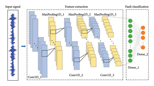
As shown in Figure 1, the network structure of the 1-D CNN consists of multiple Conv1D layers with different parameters to learn significant features from the input data. Each Conv1D layer uses filters to perform convolutions and extract local patterns and features. Following each Conv1D layer, a MaxPooling1D layer is added to reduce the spatial dimensions of the data. To transition from the last MaxPooling1D layer to the fully connected layers, a flattening layer is employed. The dense layers that follow are fully connected and utilize suitable activation functions for the classification task. The output layer utilizes a Softmax classifier to produce probability distributions across the potential health conditions.
3.3. Structural Parameter Settings
In this study, the structural parameters for training the designed 1-D CNN model were systematically determined via grid search with 10-fold cross-validation [42]. The detailed configurations for each layer of the network are presented in Table 1.
| Layer | Filters | Kernel size | Stride | Activation function | Padding |
|---|---|---|---|---|---|
| Conv1D_1 | 16 | 3 | 1 | ReLU | — |
| MaxPooling1D_1 | — | 2 | — | — | — |
| Conv1D_2 | 32 | 3 | 1 | ReLU | Same |
| MaxPooling1D_2 | — | 2 | — | — | — |
| Conv1D_3 | 64 | 3 | 1 | ReLU | Same |
| MaxPooling1D_3 | — | 2 | — | — | — |
| Flatten | — | — | — | — | — |
| Dense_1 | 256 | — | — | ReLU | — |
| Dense_2 | 10 | — | — | Softmax | — |
In addition to the structural parameters, the training hyperparameters were also determined through grid search with 10-fold cross-validation. These hyperparameters include the optimizer, learning rate, batch size, number of epochs, and loss function, as detailed in Table 2.
| Optimizer | Learning rate | Batch size | Epochs | Loss function |
|---|---|---|---|---|
| ADAM | 0.001 | 256 | 100 | Cross-entropy |
It is important to note that dropout regularization with a rate of 0.2 is applied to the first fully connected layer (Dense_1) to enhance the generalization ability of the model. In addition, batch normalization is utilized on the outputs of Dense_1 to accelerate convergence, reduce internal covariate shift, and stabilize gradient flow. This comprehensive approach to parameter and hyperparameter optimization ensures that the model is well suited for effectively diagnosing faults in rotating machinery based on vibration signals.
3.4. Training of the 1-D CNN
-
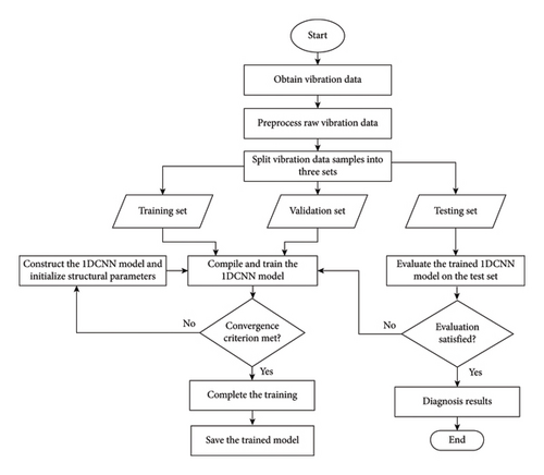
Step 1: the training data are processed and formatted to meet the input requirements of the 1-D CNN model. This encompass data initialization, preprocessing (such as normalization or scaling), and label conversion to ensure that the input is compatible with the model architecture.
-
Step 2: the 1-D CNN model is constructed and initialized with selected structural parameters, which are determined through grid search with k-fold cross-validation. These parameters consist of configurations for Conv1D layers, MaxPooling1D layers, kernel sizes, activation functions, and the number of neurons in the dense layers.
-
Step 3: the 1-D CNN model is compiled via the Adam optimizer, with a learning rate of 0.001. Categorical cross-entropy is designated as the loss function, and accuracy is used as the evaluation metric.
-
Step 4: the model is trained via the fit method. The training data, corresponding labels, number of epochs, batch size, and validation data are provided as inputs. The training progress is displayed for each epoch by setting the verbose parameter to 1.
-
Step 5: the training process continues until a convergence criterion is met. This criterion could reach a certain number of epochs, achieve the desired level of accuracy, or yield a minimal improvement in the loss function. If the convergence criterion is not satisfied, the process returns to Step 2 to adjust the structural parameters of the model and retrain.
-
Step 6: once the desired convergence criterion is met, the performance of the model is evaluated on the test set to evaluate its diagnostic capabilities on unseen data. If the evaluation results are unsatisfactory, the process reverts to Step 3 to adjust training parameters and retrain the model.
By adhering to these procedures, the 1-D CNN model is effectively trained and evaluated for its diagnostic performance on the test set. The training and testing workflows of the 1-D CNN-based fault diagnosis system for rotating machinery are depicted in Figure 2.
4. Experimental Validation
In this section, the experimental validation of the proposed adaptive 1-D CNN-based fault diagnosis method is presented. Comparative experiments and analyses are then conducted with existing CNN-based diagnosis methods to demonstrate its superiority. The practical implications of the findings are also discussed.
4.1. Data Description
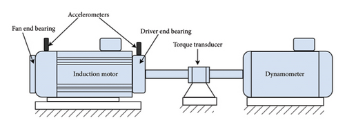
The rolling bearing vibration data utilized in this study were obtained from CWRU [22]. The experimental setup consists of a 2 hp induction motor, a torque transducer/encoder, a dynamometer, and a control circuit, as shown in Figure 3.
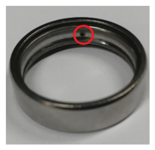
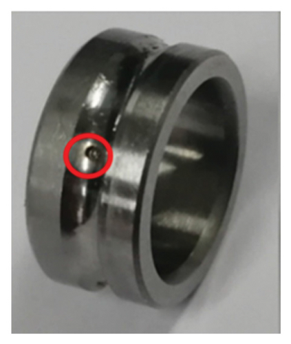
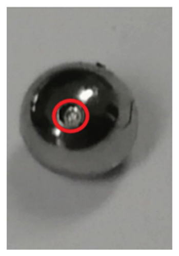
For this study, the vibration signals from the drive end bearings sampled at 12 kHz were chosen. The data were collected under four different bearing conditions: healthy, outer ring fault, inner ring fault, and ball fault. The locations of these bearing faults are shown in Figure 4. The bearing defects were intentionally introduced using electrodischarge machining, with three diameters: 0.007, 0.014, and 0.021 inches. This results in a total of 10 conditions: nine fault conditions and one healthy condition. To account the varying working conditions in practical scenarios, the data were also collected at four different load conditions: 0 hp at 1797 rpm, 1 hp at 1772 rpm, 2 hp at 1750 rpm, and 3 hp at 1730 rpm.
4.2. Data Preparation and Preprocessing
For this study, four datasets were prepared (i.e., A, B, C, and D) corresponding to 0, 1, 2, and 3 hp, respectively. Each dataset encompasses 10 bearing conditions, as previously described. To further evaluate the diagnostic performance under varying operating conditions, a combined dataset, A/B/C/D, was also created. The details of the datasets are presented in Table 3.
| Dataset | Working conditions | Number of classes | Labels | |
|---|---|---|---|---|
| Load (hp) | Rotating speed (rpm) | |||
| A | 0 | 1797 | 10 | 0/1/2/3/4/5/6/7/8/9 |
| B | 1 | 1772 | 10 | 0/1/2/3/4/5/6/7/8/9 |
| C | 2 | 1750 | 10 | 0/1/2/3/4/5/6/7/8/9 |
| D | 3 | 1730 | 10 | 0/1/2/3/4/5/6/7/8/9 |
| A/B/C/D | Combined | Combined | 10 | 0/1/2/3/4/5/6/7/8/9 |
Figure 5 shows raw time-domain vibration signals for each bearing condition at 0 hp. The signals exhibit distinct characteristics associated with each state: healthy, outer ring fault, inner ring fault, and ball fault.

To ensure the quality of the input vibration data before feeding it into the 1-D CNN, a preprocessing step was implemented using a preprocessor class. This class employs the Min–Max scaling technique to normalize the feature values to a uniform range, typically between 0 and 1 [43, 44]. This process improves the performance and convergence speed of the neural network by ensuring that all input features contribute equally to the learning process.
In this specific implementation of the preprocessing step, the fit transform method is applied to the training set, while the transform method is used for the test and validation sets. This approach guarantees consistent scaling across all datasets, which is essential for maintaining the integrity of model evaluation and enhancing the model’s ability to generalize to unseen data.
4.3. Data Augmentation
To improve the generalization performance of deep learning models, increasing the number of training samples is essential [45]. In this study, data augmentation was applied using an overlapping algorithm. This method involves overlapping segments of the one-dimensional time-domain vibration signal during sampling, where each segment overlaps with the next. This process is shown in Figure 6.
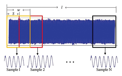
The details of the overlapping algorithm used to generate training, validation, and testing samples are outlined in Algorithm 2.
-
Algorithm 2: Overlapping algorithm to generate training, validation, and testing samples.
-
Function:generate_samples(Sig, w, S)
-
Input: Given a long signal Sig, w = 2048, S = 64
-
Output: Training samples, validation samples, and testing samples
-
Begin
-
Initialize variables:
-
Let l = len(Sig)
-
Calculate the total number of overlapping samples N:
-
N = int((l − w)/S) + 1
-
Calculate the number of samples for each set:
-
Ntrain = int(0.7 × N)
-
Nval = int(0.15 × N)
-
Ntest = N − Ntrain − Nval
-
Initialize lists:
-
train_samples = []
-
val_samples = []
-
test_samples = []
-
Extract overlapping samples:
-
Fori = 0 to N − 1do:
-
start_index = i × S
-
end_index = start_index + w
-
sample = Sig[start_index : end_index]
-
Distribute sample into datasets based on index:
-
ifi < Ntrainthen:
-
append sample to train_samples
-
else ifi < Ntrain + Nvalthen:
-
append sample to val_samples
-
else:
-
append sample to test_samples
-
End for
-
Return train_samples, val_samples, and test_samples.
-
End
4.4. Result Analysis
This subsection presents the results of the Bayesian optimization process. Following this, the diagnostic results of the 1-D CNN model utilizing the optimized parameters are analyzed.
4.4.1. Optimization Results
The main contribution of this study is the introduction of a Bayesian optimization algorithm that adaptively identifies the optimal combination of input parameters in vibration signal analysis for a 1-D CNN-based fault diagnosis method. The search space for each parameter is established based on insights from a theoretical formula and a thorough literature review. For instance, the data points acquired per rotation are derived from the sampling frequency and rotation speed. The formula used to calculate the data points per rotation is as follows: sampling count per circle = sampling frequency × 60/rotating speed [47]. For dataset A, where the vibration signal was collected at 1797 rpm, the minimum data points for each sample were calculated as follows: data points = 12,000 × 60/1797 = 400. Consequently, the search space for the data point parameters in this study is set between 400 and 10,000 for all datasets. The search space for the data augmentation stride parameter ranges from 1 to 200, where a stride of 1 indicates that augmented data are generated without any gaps between the original data points. In addition, the train set numbers vary between 100 and 1,000, while the validation set numbers range from 5 to 250. The test set numbers are explored within a range of 10–500.
Considering these defined search spaces, the Bayesian optimization process adaptively yields the optimal parameters that can enhance the diagnostic accuracy of the 1-D CNN, as presented in Table 4.
| Dataset | Number of samples | Data points per sample | Stride | ||
|---|---|---|---|---|---|
| Train set | Validation set | Test set | |||
| A | 1000 | 120 | 480 | 3727 | 121 |
| B | 715 | 110 | 324 | 8029 | 170 |
| C | 742 | 85 | 357 | 7057 | 163 |
| D | 650 | 144 | 339 | 9584 | 180 |
| A/B/C/D | 1297 | 186 | 527 | 4896 | 137 |
It is evident from Table 4 that the optimization results vary for different datasets due to the adaptive nature of the presented optimization method. For dataset A, a total of 1600 samples are allocated, with 1000 samples designated for training (approximately 62.5%), 120 samples for validation (around 7.5%), and 480 samples for testing (about 30%). This distribution pattern is consistent across other datasets, with approximately 60%–65% of the data allocated to the training set, while the validation and testing sets account for about 7%–12% and 26%–30%, respectively. Such a systematic allocation aligns with established trends in model training, where the training set is larger than the testing set, which in turn is larger than the validation set. This distribution ensures effective model training and evaluation, optimizing performance across various datasets.
Regarding the length of each sample, dataset A is set to 3727 data points, dataset B to 8029 data points, dataset C to 7057 data points, dataset D to 9584 data points, and the combined dataset A/B/C/D to 4869 data points. Interestingly, the findings from the study challenge the conventional belief that data points within each sample must conform to a power-of-2 format to achieve optimal accuracy in diagnostic procedures. The results suggest that optimal diagnostic accuracy can be achieved even without conforming to a power-of-2 format for the data points within each sample. This observation challenges the long-standing assumption that power-of-2 sampling universally guarantees the best diagnostic accuracy.
Moreover, the data augmentation stride used in the study is set to 121, 170, 163, 180, and 137 for datasets A, B, C, D, and the combined dataset A/B/C/D, respectively. These input parameters are employed as inputs for a 1-D CNN model to achieve accurate and reliable fault diagnosis.
4.4.2. Diagnosis Results
Once the optimal input parameters are determined, the proposed 1-D CNN model is trained on the training and validation sets, and the performance of the trained model is subsequently assessed on the test set. Before the testing results are presented, it is crucial to evaluate the convergence of the training process. This assessment helps determine whether the model has reached a stable state and is no longer significantly improving its performance. The model is trained for 100 epochs. To ensure result reliability, the experiment is repeated 10 times for each dataset. Figure 7 provides a detailed visualization of the training accuracy and loss curves for each dataset within a single trial.
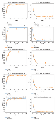
Upon analyzing Figure 7, it becomes evident that both the training and validation accuracies for all the datasets reach 100% after approximately 20 epochs. This achievement signifies that the 1-D CNN model, with its optimized parameters, effectively learned and adjusted its parameters during training. Moreover, both the training and validation losses consistently decrease and converge to 0, indicating a stable pattern around the same epoch. This convergence indicates that the training process has reached a point where further iterations would yield minimal changes to the loss, suggesting that the model has successfully captured the underlying patterns and features in the data. The smoothness of the training process further supports its ability to minimize loss and improve performance. These findings, including high accuracy, stable loss function, and a smooth training process, provide strong evidence of the successful training and optimization of the 1-D CNN model. The careful determination of optimal combinations of key input parameters, such as sample size, the number of data points within each sample, and the data augmentation stride in vibration signals, likely contributed to this success. Overall, these findings highlight the successful training and optimization of the 1-D CNN model, confirming its ability to reliably detect fault patterns in the given datasets.
After the training process is complete, the fault diagnosis accuracy of the trained model is evaluated on the test set. The results prove that the 1-D CNN model achieves an accuracy rate of 100% on each dataset, including the combined dataset A/B/C/D. The remarkable accuracy rate can be attributed to the utilization of optimized input parameters. The systematic determination of these parameters has significantly contributed to the success of the 1-D CNN model in fault diagnosis of vibration signals in the time domain. By finding the optimal combinations, the model was able to capture and analyze the relevant patterns and features in the data effectively, leading to highly accurate and reliable diagnosis results. Overall, the proposed method exhibits excellent performance in terms of diagnostic accuracy and reliability.
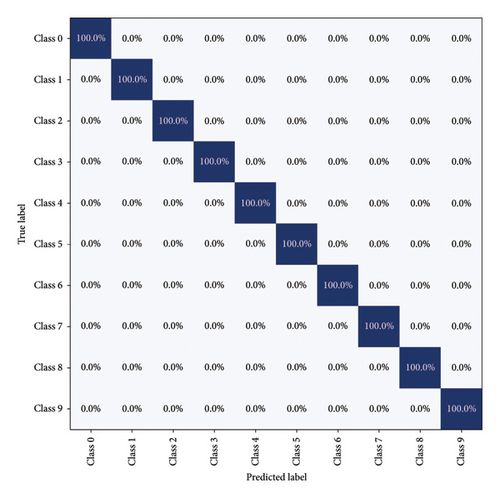
To provide a clearer insight into the diagnostic accuracy of each class in the testing set by the 1-D CNN model, a multiclassification confusion matrix is employed. As shown in Figure 8, the 1-D CNN model, optimized with input parameters, achieves a 100% accuracy rate in identifying the 10 different conditions within the testing set, irrespective of consistent or changing operational conditions. This outcome leads to the conclusion that the 1-D CNN model presented here effectively detects faults in bearings operating under intricate working conditions.
To investigate the feature learning capabilities of the 1-D CNN model, t-distributed stochastic neighbor embedding (t-SNE) is utilized to visualize the learned features from the test samples. In a single trial using the combined dataset A/B/C/D, the features learned from each convolutional layer and the dense layers of the model are projected into two-dimensional (2-D) representations. The visualization results, presented in Figure 9, exhibit the distributions of these features in a 2-D scatter plot.
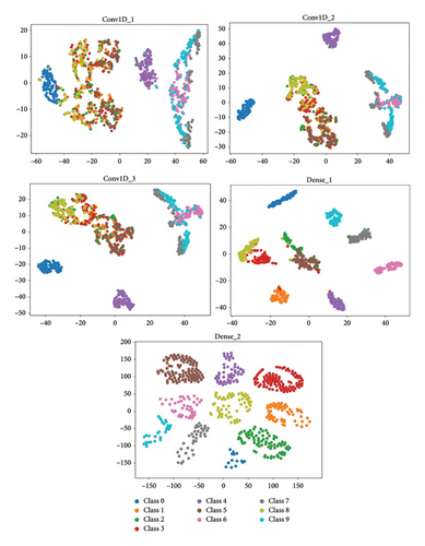
The visualization in Figure 9 reveals that as the number of hidden layers increases, the overlapping areas among different categories gradually decrease. Particularly at the final fully connected layer (dense_2), minimal misclassification is observed. These findings suggest that the constructed 1-D CNN model has strong feature learning capabilities, leading to excellent classification performance. The ability of the model to reduce overlapping regions and minimize misclassifications demonstrates its practicality and effectiveness in diagnosing faults in rolling bearings within rotating machinery.
4.5. Comparative Experiments and Analysis With Other Methods
To further delineate the efficacy of the presented 1-D CNN model with optimized parameters, comparative experiments and analyses are performed with existing CNN-based fault diagnosis methods, considering varying load conditions. These methods include CNN [17], two-dimensional convolutional neural network (2D-CNN) [48], multiscale deep convolutional neural network (MS-DCNN) [47], and deep convolutional neural networks with wide first-layer kernels (WDCNN) [18]. These architectures were chosen to represent a spectrum of CNN designs used in fault diagnosis and to leverage proven performance in prior studies.
To ensure statistical reliability and minimize the impact of random initialization, 10 independent trials were performed for each method. The average fault diagnosis accuracies and corresponding standard deviations obtained from these trials are presented in Table 5. This approach offers a robust comparison of model performance under varying load conditions.
| Method | Diagnosis accuracy (%) |
|---|---|
| CNN | 96.96 ± 1.36 |
| 2D-CNN | 98.25 ± 0.41 |
| MS-DCNN | 99.27 ± 0.23 |
| WDCNN | 100 ± 0 |
| Proposed 1-D CNN | 100 ± 0 |
As presented in Table 5, the CNN model attains the lowest average diagnosis accuracy of 96.96% with a relatively high standard deviation of 1.36%. This suggests that the performance of the CNN model in fault diagnosis is less consistent, leading to varying results. In contrast, the 2D-CNN model achieves a higher average accuracy of approximately 98.25% with a lower standard deviation of 0.41%. This indicates a more consistent and reliable fault diagnosis than the CNN model does. The MS-DCNN model further improves the accuracy, achieving an average accuracy of 99.27% with a minimal standard deviation of 0.23%. These results demonstrate the robustness of the MS-DCNN model, as it consistently performs well across different load conditions. Both the WDCNN and the proposed 1-D CNN models with optimized input parameters achieve a perfect diagnosis accuracy of 100% without any standard deviation. Interestingly, the training process of the proposed 1-D CNN model is smoother than that of the WDCNN model. This enhanced stability and convergence during training can be attributed to the implementation of batch normalization. As a result, the presented 1-D CNN demonstrates better convergence and stability, leading to consistent diagnostic performance during testing.
4.6. Practical Implications
The fault diagnosis method presented in this study has significant practical implications and potential applications in the field of fault diagnosis. First, the ability of the proposed deep learning-based fault diagnosis method to achieve a high accuracy rate and a smooth training process through optimizing input parameters in vibration signal analysis enables its effective utilization with various datasets and rotating machines. This versatility allows the method to be applied in practical scenarios where multiple datasets with varying characteristics and diverse equipment are encountered. Second, the optimization of the structural parameters of the proposed deep learning model is achieved through a grid search with a k-fold cross-validation strategy. This approach takes into consideration the unique characteristics of the dataset and research objects. As a result, the method is well suited for practical applications, as it takes into account the specific requirements and variations of the dataset and mechanical equipment being analyzed. Furthermore, the effectiveness of the proposed method is demonstrated not only under constant working conditions but also under variable working conditions. This expands its practical usefulness, as many real-world systems operate in dynamic and changing environments. By effectively handling variable working conditions, the method can be applied in scenarios where the operational parameters may fluctuate. This ensures accurate fault diagnosis, even in complex and dynamic systems. However, it is important to consider the computational resources and time necessary for training and optimization when implementing the deep learning-based diagnosis method. The practical implementation of the diagnosis method should align with the available computational infrastructure to ensure feasibility and efficiency.
5. Conclusion and Future Recommendations
In this paper, an adaptive method based on a Bayesian optimization algorithm is presented to identify the optimal combination of the number of samples, data points per sample, and data augmentation stride for vibration signal analysis. The primary objective of this study was to improve the accuracy of a 1-D CNN-based fault diagnosis method in rotating machines. The proposed adaptive method was validated using vibration signals collected from motor rolling bearings and achieved a diagnosis accuracy of 100%. The main contribution of this study is the ability of the proposed method to eliminate the manual selection inherent in traditional approaches by adaptively determining the input parameters in vibration signal analysis tailored to specific fault diagnosis tasks.
In comparison with other CNN-based methods, the method presented in this paper has superior diagnostic performance and generalization capability, particularly in scenarios characterized by variable operating conditions. This robustness to varying working conditions proves the practicality of the proposed adaptive 1-D CNN-based fault diagnosis method in real-world applications. In addition to achieving the highest accuracy, the presented method consistently showed stable training processes, indicating its robustness and reliability.
Although the present study indicates that optimizing sample size, data points per sample, and data augmentation stride in vibration signal analysis can improve the accuracy of deep learning-based fault diagnosis, further research is needed to fully understand the impact of sample size on this accuracy. It is important to examine how variations in sample size affect the robustness and reliability of deep learning models. This will be essential for developing more dependable fault diagnosis systems. Moreover, it is important to investigate optimal sample sizes and other data parameters beyond vibration signals. Investigating the optimal number of samples required for temperature, acoustic signals, wear debris, and other data types can provide a more comprehensive understanding of the applicability of deep learning models in diverse fault diagnosis scenarios. This broader exploration will strengthen the foundations for building more reliable and versatile deep learning-based fault diagnosis systems for rotating machinery.
Conflicts of Interest
The authors declare no conflicts of interest.
Funding
This work was supported by the Artificial Intelligence and Robotics Center of Excellence at Addis Ababa Science and Technology University (grant number IGP012/2023).
Acknowledgments
We would like to thank the anonymous reviewers for their comments, which greatly improved the quality of the paper.
Open Research
Data Availability Statement
The data that support the findings of this study are available from the corresponding author upon reasonable request.


