Volume 2025, Issue 1 5446251

Research Article

Open Access

Response Surface Model Optimization Algorithm for Structural Assessment Based on Vibration Frequency

Xiao-Guang Wang,

Corresponding Author

Xiao-Guang Wang

[email protected]

orcid.org/0000-0003-4622-2605

School of Highway , Chang’an University , Xi’an , 710064 , Shaanxi, China , chd.edu.cn

CCCC First Highway Consultants Co., Ltd , Xi’an , 710000 , Shanxi, China , ccccltd.cn

Search for more papers by this author

Ming M. A.,

Ming M. A.

CCCC First Highway Consultants Co., Ltd , Xi’an , 710000 , Shanxi, China , ccccltd.cn

Search for more papers by this author

Bin Zhao,

Bin Zhao

School of Civil Engineering , Qingdao University of Technology , Qingdao , 266520 , Shandong, China , qust.edu.cn

Search for more papers by this author

Wen-Hao Zhang,

Wen-Hao Zhang

School of Civil Engineering , Qingdao University of Technology , Qingdao , 266520 , Shandong, China , qust.edu.cn

Search for more papers by this author

Shuai Song,

Shuai Song

orcid.org/0000-0001-6512-9030

School of Civil Engineering , Qingdao University of Technology , Qingdao , 266520 , Shandong, China , qust.edu.cn

Search for more papers by this author

Xiao-Guang Wang,

Corresponding Author

Xiao-Guang Wang

[email protected]

orcid.org/0000-0003-4622-2605

School of Highway , Chang’an University , Xi’an , 710064 , Shaanxi, China , chd.edu.cn

CCCC First Highway Consultants Co., Ltd , Xi’an , 710000 , Shanxi, China , ccccltd.cn

Search for more papers by this author

Ming M. A.,

Ming M. A.

CCCC First Highway Consultants Co., Ltd , Xi’an , 710000 , Shanxi, China , ccccltd.cn

Search for more papers by this author

Bin Zhao,

Bin Zhao

School of Civil Engineering , Qingdao University of Technology , Qingdao , 266520 , Shandong, China , qust.edu.cn

Search for more papers by this author

Wen-Hao Zhang,

Wen-Hao Zhang

School of Civil Engineering , Qingdao University of Technology , Qingdao , 266520 , Shandong, China , qust.edu.cn

Search for more papers by this author

Shuai Song,

Shuai Song

orcid.org/0000-0001-6512-9030

School of Civil Engineering , Qingdao University of Technology , Qingdao , 266520 , Shandong, China , qust.edu.cn

Search for more papers by this author

First published: 17 March 2025

https://doi.org/10.1155/vib/5446251

Academic Editor: Iacopo Tamellin

Share a link

Email
Wechat
Bluesky

Abstract

Finite element model modification based on response surface method is an effective engineering method that can significantly improve the accuracy of finite element model and structural evaluation. In order to solve the shortcomings of the response surface method based finite element model correction, which exists that the polynomial order selection rule is unknown and the correction result is easily affected by the quality of the optimization target, based on the relationship between the polynomial order and the response surface accuracy and computation amount, a robust estimation algorithm was introduced to optimize the response surface solution process, which improves the reliability of the response surface based model correction. Taking an actual project of a cable-stayed bridge as an example, the response surface-based finite element model modification method was adopted to compare the response surface accuracy and computation amount of three kinds of response surface models, namely, second-mode polynomials, third-mode polynomials and fourth-mode polynomials. The optimization results of the robust estimation method were compared with the traditional solution method under the conditions of large fluctuation and small fluctuation of optimization target between finite element index. The results show that with the increase of the polynomial order of the response surface model, the unknown covariates to be solved in the response surface model increase sharply, which increases the computational cost, but the effect of improving the accuracy of the response surface model is limited. When the target frequency fluctuates greatly, compared with the least-squares method, robust estimation will not transfer the error of the correction result of the order with the large fluctuation of the index difference to the other orders, which ensures the stability of the correction results.

1. Introduction

Due to the variability of actual materials and the randomness during construction, there exists a significant difference between finite element models and actual bridge structures [1, 2]. In addition, with the increase of service time, there is a performance degradation problem of bridge structural materials such as concrete [3, 4]. The actual operating condition of the bridge differs from the design condition [5]. The design finite element model of the bridge differs from the actual structure in terms of structural static and dynamic response [6]. A reasonable finite element model is needed for structural analysis and evaluation [7, 8]. Finite element model modification is the foundation in the assessment of bridge [9].

Finite element model modification has undergone a development process from matrices to parameters, from low-dimensional to high-dimensional, from dynamic response to static or combined static-dynamic response [10], from local solving to global optimization, and from determinism to uncertainty [11–13]. Various new model modification methods are proposed [14–16]. Among all the model modification methods, the surrogate model modification method based on response surface method is widely adopted by researchers due to its advantages of high accuracy and efficiency [17]. The most widely used model is the response surface model established based on polynomials [18, 19]. However, there is currently little research on polynomial order selection and model accuracy, making it difficult to accurately grasp the specific rules for establishing polynomials in practical applications [20].

The finite element model modification based on response surface takes the structural dynamic or static-dynamic test results as the optimization objective [21–23]. The variation of finite element model parameters is obtained by solving the established response surface model and the purpose of modifying the finite element model is achieved [24, 25]. Most model modification processes take bridge modal parameters as the modification objective [26–28]. Bridge modal parameters are generally obtained by analyzing bridge vibration acceleration data [29]. Due to environmental disturbances and other factors, the actual identified bridge structural modal parameters often differ from the finite element results, with some modal orders having significant differences while others having minor differences [30]. Existing model modification methods often focus on the modification process itself, neglecting the differences between the optimization objectives and the finite element results [31, 32]. They adopt generic methods to handle the iterative optimization problems in the modification process, making it difficult to control local errors and easily propagate errors of orders with significant differences to other orders, thereby affecting the modification results of other orders [33, 34].

The issue of polynomial order selection in existing response surface-based finite element model modification processes was addressed in this study. The robust estimation method was introduced into the optimization solution process of the response surface model to solve the error transmission problem. The indicator error is locally controlled. Based on a cable-stayed bridge, the finite element model modification process based on the response surface method was used to analyze the relationship between polynomial order and response surface accuracy as well as computational amount, providing guidance for response surface model establishment. When the optimization target fluctuates greatly, better correction results can still be obtained to ensure the correction accuracy of the model correction.

2. Finite Element Model Modification Based on Response Surface

2.1. Response Surface Methodology (RSM)

RSM is a statistical method that utilizes reasonable experimental design methods and obtains certain data through experiments, and adopts multivariate quadratic regression equations to fit the functional relationship between the factors and the response values, and seeks for the optimal parameters and solves the multivariate problems by analyzing the regression equations. The response surface method is widely used in optimization problems where the relationship between the influencing factors and the response is not shown. The main steps of RSM include experimental design, data collection, model fitting, response surface analysis, optimization and validation.

2.2. Model Modification Based on Response Surface

To improve computational efficiency and visualize the relationship between modification parameters and results, response surface models are used for bridge structural model modification. By establishing response surface models between structural parameters and structural frequency response, the repetitive process of calling finite element calculations is avoided. The finite element model modification based on response surface includes four steps: parameter sensitivity analysis and significance testing, response surface fitting, response surface accuracy testing, and optimization solution.

2.2.1. Parameter Sensitivity Analysis and Significance Testing

The purpose of parameter sensitivity analysis is to select the parameters for modification. Through parameter sensitivity analysis, parameters that have a significant impact on the modification results are selected as the parameters for modification, while parameters with a minor impact are excluded. After selecting the parameters for modification and completing the experimental design, significance testing methods are used to determine the parameters and parameter combinations involved in the polynomial response surface fitting. Parameter sensitivity analysis and significance testing ensure that the number of parameters to be solved in the response surface model is reduced without affecting the modification results. Then, the computational burden of solving the response surface model is greatly reduced.

Sensitivity analysis typically adopts the following indicators:

\begin{matrix} S_{i j}^{f} = (\frac{({f_{j}}^{'} - f_{j}^{0}) / f_{i}^{0}}{(x_{i}^{1} - x_{i}^{0}) x_{i}}) = \frac{(Δ f_{j} / f_{j}^{0})}{(Δ x_{i} / x_{i}^{0})}, (i = 1212,, \dots, n, j =,, \dots, m), \end{matrix}

()

where

S_{i j}^{f}

is the sensitivity of the j response feature to parameter x_i;

x_{i}^{0}

and

x_{i}^{1}

are the parameter values of the two calculations;

f_{j}^{0}

and

f_{j}^{1}

are the j response values of the two calculations; n is the total number of parameters and m is the total number of response features, which is determined by the actual data collected. Significance testing generally uses F-test. The significance level values of the parameter are calculated. The parameters that have a significant impact on the structural response are then screened out by testing the hypotheses. The significance level indicator is calculated with equation (2).

\begin{matrix} F_{m} = \frac{S S E (x_{1}, x_{2}, x_{3}, \dots, x_{m - 1}) - SSE (x_{1}, x_{2}, x_{3}, \dots, x_{m - 1}, x_{m})}{S S E (x_{1}, x_{2}, x_{3}, \dots, x_{m - 1}, x_{m}) / (n - m - 1)}, \end{matrix}

()

where SSE(x₁, x₂, x₃, …, x_m−1) is the sum of squares of the errors of the regression model of x₁, x₂, x₃, …, x_m−1, SSE(x₁, x₂, x₃, …, x_m−1, x_m) is the sum of squared of the errors of the regression model of x₁, x₂, x₃, …, x_m−1, x_m, n is the total number of parameters.

Generally, given a critical significance level α = 0.05, if the sample parameter probability is p ≤ 0.05, the effect of the eigenvalue is significant and should be involved in the response surface fitting. Otherwise, it is considered insignificant and the parameter combination is not used in the response surface fitting.

2.2.2. Response Surface Fitting

The purpose of response surface fitting is to establish an explicit relationship between the modified parameters and the structural response. Polynomial functions, radial basis functions, and nonlinear functions are the commonly used functions for the response surface model. The second-order polynomial form of the response surface model is expressed in equation (3).

\begin{matrix} y = β_{0} + \sum_{i = 1}^{k} β_{i} x_{i} + \sum_{i = 1}^{k} β_{i j} x_{i}^{2} + \sum_{i} \sum_{i = 1}^{k} β_{i j} x_{i} x_{j}, \end{matrix}

()

where β₀, β_i, β_ii, β_ij are the undetermined coefficients.

The selection of the order of the response surface model is the key to the finite element model modification based on the response surface. A lower-order polynomial model may cause low accuracy of the response surface model. A higher-order polynomial model leads to the number of coefficient parameters in the response surface model increases significantly, then the computational complexity significantly increased. Therefore, choosing an appropriate polynomial order is crucial for balancing solution accuracy and efficiency.

2.2.3. Response Surface Accuracy Testing

The purpose of response surface model accuracy testing is to determine whether the fitting accuracy of the response surface model meets the requirements and whether it can represent the real response of the structure. A limited number of sample points are randomly selected in the entire design space. The sample points of the initial experimental design should be avoided. The selected sample points are then substituted into the finite element model and the fitted model respectively to obtain the corresponding response characteristic values. The fitting effect of the response surface can be assessed using multiple correlation coefficient (R²) and root mean square error (RMSE). The expression of R² is equation (4) and the expression of RMSE is equation (5).

\begin{matrix} R^{2} = 1 - \frac{\sum_{j = 1}^{N} {[y_{R S} (j) - y (j)]}^{2}}{\sum_{j = 1}^{N} {[y (j) - \bar{y}]}^{2}}, \end{matrix}

()

\begin{matrix} RMSE = \frac{1}{N \bar{y}} \sqrt{\sum {[y_{R S} (j) - y (j)]}^{2}}, \end{matrix}

()

where N is the number of sample points to be tested; y_RS(j) is the value of the response surface model for the j sample point, y(j) is the finite element model response for the j sample point, and

\bar{y}

is the average value of all the sample points. The calculation results of the test are between 0 and 1. If the value of R² is close to 1 and the value of RMSE is close to 0, the response surface model is good, and it can reflect the original model characteristics. If the test results are not satisfactory, the response surface fitting needs to be restarted from the beginning.

2.2.4. Response Surface Optimization

Response surface optimization is the constrained optimization of the response surface equation set within the parameter setting range through optimization algorithms. It can be expressed by the following mathematical model.

\begin{matrix} \{\begin{matrix} Min F (x), \\ F (x) = {\sum (\{f_{\exp}\} - \{f_{RSM}\})}^{2}, \\ l b \leq x \leq u b, \end{matrix} \end{matrix}

()

where F(x) is the residual function between the measured response and the response surface model, f_exp represents the measured response, f_RSM represents the structural response obtained from the response surface model, and lb, ub are the lower and upper bounds of x. Least squares method can be used to solve equation (6).

3. Robust Estimation Method

In dynamic model modification, with the actual modal parameters of bridge structures serving as optimization objectives, the monitoring data during the operation of bridges often contain various unquantifiable interfering factors. The modal parameters of bridges obtained based on monitoring data probably exhibit strong discreteness, and the deviations between each-order correction objective and finite element results are unevenly distributed. Existing correction methods treat each-order objective function uniformly during the correction process. Inevitably, the effect of a large deviation in one order will be passed on to other orders, thus affecting the overall correction result. To control the degree of error influence on correction objectives and ensure that the modification results are not significantly affected by modal parameter indicators with large deviations, a response surface model optimization method based on robust estimation is proposed.

Robust estimation can address the problem of overall deviation of optimization results caused by outliers in observed values. Through robust estimation, accurate estimates can be obtained when the deviation between observed values and target values is small, and the performance of parameter estimates will not be too poor when the deviation between observed values and ideal values is large. The commonly used robust estimation method is M-estimation, which defines a weighting function ρ to weight different observed values and then obtains the best estimate of the parameters. The process is as follows.

The observed value is expressed with L, the vector of unknown parameters is

\overset{\land}{X}

, and the observation equation is equation (7).

\begin{matrix} V = A \overset{\land}{X} - L = (\begin{matrix} a_{1} \\ a_{2} \\ ⋮ \\ a_{n} \end{matrix}) \overset{\land}{X} - (\begin{matrix} L_{1} \\ L_{2} \\ ⋮ \\ L_{n} \end{matrix}), \end{matrix}

()

where V is the residual vector of n dimensional measurement, A is n × m design matrix, L is the optimization objective of corresponding response surface model,

\overset{\land}{X}

is unknown parameters to be solved in the corresponding response surface model.

Prior weighted diagonal matrix P is expressed with equation (8).

\begin{matrix} P = [\begin{matrix} p_{1} & 0 & \dots & 0 \\ 0 & p_{2} & \dots & 0 \\ ⋮ & ⋮ & ⋱ & 0 \\ 0 & 0 & 0 & p_{n} \end{matrix}] . \end{matrix}

()

M estimation uses the idea of great likelihood estimation, which maximizes the probability density of the joint occurrence of a set of small independent errors. The expression is equation (9).

\begin{matrix} G = f (\overset{\land}{X} - L_{1}) • f (\overset{\land}{X} - L_{2}) • \dots f (\overset{\land}{X} - L_{n}) = \max . \end{matrix}

()

The equation (9) is equivalent to equation (10):

\begin{matrix} \sum_{i = 1}^{n} [- ln f (\overset{\land}{X} - L_{i})] = \min . \end{matrix}

()

Using function ρ replace −ln f, The goal of equation solving is to minimize residuals, which can be expressed as

\begin{matrix} \sum_{i = 1}^{n} ρ (ν_{i}) = \sum_{i = 1}^{n} p_{i} (a_{i} \overset{\land}{X} - L_{i}) = \min . \end{matrix}

()

Take the derivative of equation (11) for x and set it to 0:

\begin{matrix} \{\begin{matrix} ϕ (ν_{j}) = \frac{\partial ρ}{\partial ν_{i}} \\ \sum_{i = 1}^{n} ρ_{i} ϕ (ν_{i}) a_{i} = 0 \end{matrix}\}, \end{matrix}

()

ϕ(ν_i)/ν_i = w_i (weighting factor),

\bar{p_{i i}} = p_{i} w_{i}

are weight elements, equation (12) is transformed to equation (13).

\begin{matrix} A^{T} P V = 0 . \end{matrix}

()

Therefore, the iterative equation of equation (6) can be expressed as

\begin{matrix} A^{T} P A \overset{\land}{X} - A^{T} P L = 0 . \end{matrix}

()

The weight matrix for each adjustment is

\begin{matrix} P (v) = diag [P_{1} (ν_{1}) P_{2} (ν_{2}) \cdot \cdot \cdot P_{n} (ν_{n})], \end{matrix}

()

P(v) is a weight matrix, if P(v) it is a constant matrix, then the parameter estimate obtained from the M estimation process is the least squares estimate.

The estimated value of the parameters obtained from the M estimation is expressed with equation (16).

\begin{matrix} \overset{\land}{X} = {(A^{T} P A)}^{- 1} A^{T} P L . \end{matrix}

()

The equation (16) is generally solved through iterative methods, k + 1 steps iterative solution expressed with equation (17).

\begin{matrix} {\overset{\land}{X}}^{k + 1} = {(A^{T} P^{k} A)}^{- 1} A^{T} P^{k} L, \end{matrix}

()

where P^k is continuously updating weight matrices.

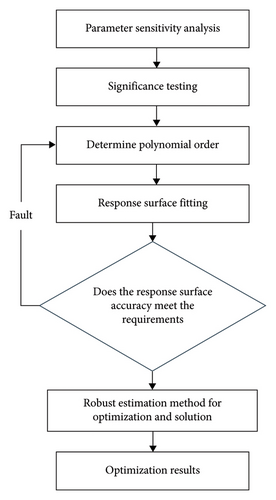
The overall process of finite element model modification based on robust estimation is shown in Figure 1.

Details are in the caption following the image — **Figure 1**
Open in figure viewer PowerPoint

Finite element model updating based on robust estimation.

4. Cable-Stayed Bridge Finite Element Model Modification

4.1. Bridge Overview

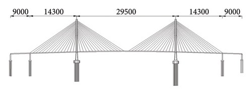
The bridge is a 90 + 143 + 295 + 143 + 90 m cable-stayed bridge with twin-tower double steel box girder. The bridge tower is a concrete tower with a height of 143 m. The shape of the bridge tower is a double-column box shape. Each bridge tower consists of two tower columns. The cross-section of the upper tower column is 4 × 4 m, and the cross-section of the lower tower column is 6 × 6 m. The bridge deck width is 26.4 m. The main tower, main pier and auxiliary pier are all made of C50 concrete, plate rubber bearing is adopted for bearing, steel strand is adopted for stay cable. Dynamic load tests were conducted when the bridge was completed to assess the dynamic performance of the bridge structure. The overview of the bridge is shown in Figure 2.

A finite element model of the bridge was established using ANSYS software (Figure 3). The main girder and main tower elements were modeled using Beam4 elements in the software, and the cables were modeled using Link8 elements. The elastic modulus of main girder, main girder density, elastic modulus of cable, cable density, and main girder area were taken as the variables for modification. The entire bridge model consists of 338 elements, including 136 main girder elements, 54 main tower elements, 28 main pier elements, and 120 stay cable elements. A spatial fishbone model was adopted to model the main girder, with all cross-sectional geometric properties and masses concentrated on the main girder. The material properties of the rigid arm elements are 10,000 times that of the steel box girder’s elastic modulus. The first five-order frequencies of the finite element model and the real bridge are listed in Table 1. In order to establish a reasonable finite element model for bridge postevaluation services, the dynamic model of the finite element model is modified taking the first five identified frequencies as correction targets.

Table 1. The frequencies of finite element model calculation and real bridge test.

Vibration modes	First mode	Second mode	Third mode	Fourth mode	Fifth mode
Measured frequency (Hz)	0.434	0.612	0.766	0.875	1.046
Finite element frequency (Hz)	0.406	0.564	0.721	0.831	1.012
Error (%)	6.45	7.84	5.87	5.03	3.25

4.2. Selection of Modification Parameters

Nine parameters influencing the structural modal response were selected as candidate parameters for the sensitivity analysis. The modal response of the bridge under various parameter change conditions are calculated with ANSYS software. The sensitivity of the nine parameters was calculated combining with MATLAB hybrid programming technology. Figure 4 shows the sensitivity of the nine parameters.

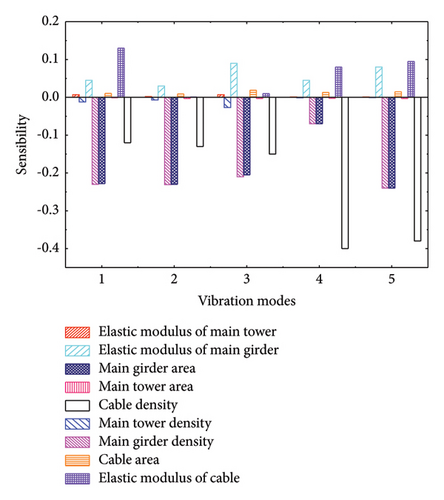
Figure 4 indicates that the influences of the elastic modulus of main tower, main tower density, main tower area, and cable area on structural frequency are relatively small. Therefore, they are not considered as parameters for modification. The effects of main girder density and main girder area on the frequencies of the five vibration modes are similar. Except for the frequency of the fourth vibration mode, they are sensitive to structural frequency. The elastic modulus of main girder is sensitive to the frequency of the third and fifth vibration modes. The elastic modulus of cable is most sensitive to the frequency of the first vibration mode. The cable density is sensitive to the frequencies of the fourth and fifth vibration modes. Therefore, the main girder density, main girder area, elastic modulus of main girder, elastic modulus of cable and cable density are selected as the five parameters for modification. A central composite design is performed with the five parameters fluctuating up and down by 30%. The ranges of values for the five parameters for modification are shown in Table 2.

Table 2. The value ranges of the five parameters for modification.

Number	Parameter	Low-level	Initial value	High-level
X₁	Elastic modulus of main girder (× 10⁵ MPa)	1.44	2.06	2.67
X₂	Main girder density (× 10³ kg/m³)	5.49	7.85	10.21
X₃	Elastic modulus of cable (× 10⁴ MPa)	1.44	2.05	2.67
X₄	Cable density (× 10³ kg/m³)	5.60	8.01	10.41
X₅	Main girder area (m²)	1.08	1.55	2.01

4.3. Experimental Design and Response Surface Fitting

A central composite design was adopted to generate parameter combination points within the range of the five parameters. One hundred sample points were obtained. The significance analyses of the one hundred sample points were conducted using F-test method to determine the significance of parameters and parameter combinations. If p value less than 0.05, the sample point has a significant impact on the response. The parameters that have a significant impact on the response were involved in polynomial fitting for response surface.

To explore the influence of polynomial order on the accuracy and computational cost of the response surface model, the significance of parameters and parameter combinations involved in two-order, three-order and four-order polynomials was calculated, respectively. The p values of the parameter combination in each regression equation were all less than 0.05, indicating strong significance of the parameter combinations. Thus, all parameter combinations should participate in polynomial fitting.

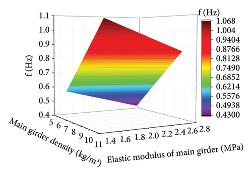
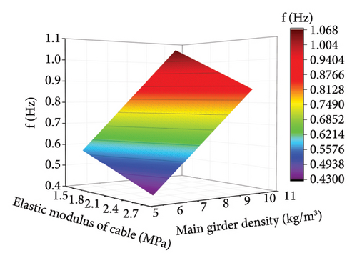
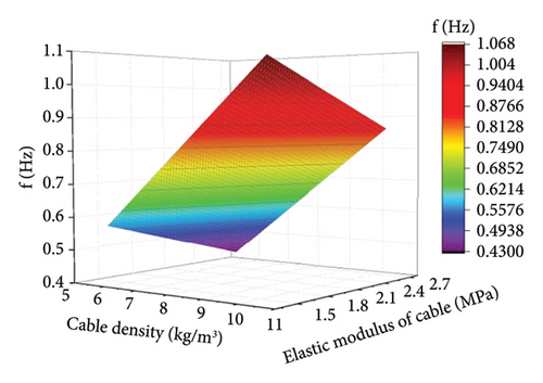
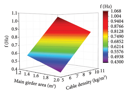
Based on the central composite design and significance analysis, response surface polynomial fitting was conducted using the obtained sample points. Due to space limitations, only the second-order response surface model of the frequency of the fifth vibration mode for selected parameters are shown in Figure 5.

The accuracy of the response surface models was tested using the R² and RMSE. Figure 6 shows the accuracy of the second-mode, third-mode, and forth-mode response surface models at different modes.

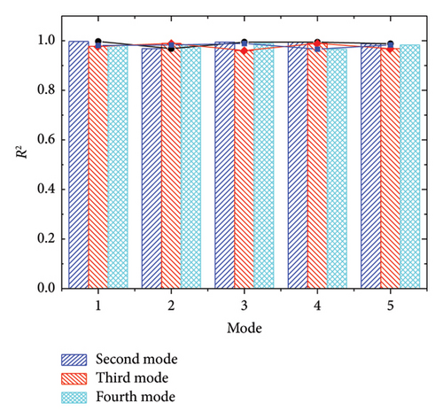
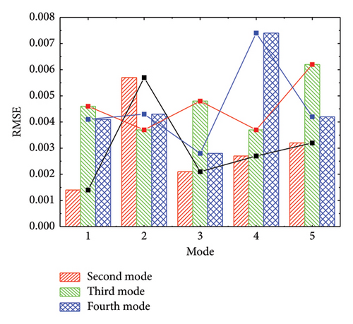
Figure 6 indicates that the R² indicators under different polynomial orders are all close to 1, and the RMSE indicators are all less than 0.008. The accuracy test results show that the precision of each order response surface model is high. However, the accuracy of response surface models at different polynomial orders did not significantly improve with the increase in polynomial order. This suggests that increasing the polynomial order may not effectively improve the fitting accuracy of the response surface. However, as the polynomial order increases, the number of unknown coefficients that need to be solved increase significantly. This not only increases the difficulty of fitting the response surface but also increases the dimensionality of the matrix during response surface optimization, which significantly increasing the difficulty and computational cost of response surface optimization. Therefore, increasing the polynomial order of the response surface does not necessarily improve the overall accuracy of the response surface but significantly increases the computational cost. When a low-order polynomial meets the requirements of accuracy, it should be prioritized for the response surface model.

4.4. Optimization of Response Surface Function

There are differences between the modal parameters of real bridges and finite element models. The differences between modal parameters identified from monitoring data of real bridges and the modal parameters calculated with finite element results are changed for different bridges. Different solving processes of the response surface handle these differences differently. The robust estimation method proposed in this study used the Huber weighting function.

The optimization results of the robust estimation method and the least squares method were compared and listed in Table 3.

Table 3. Comparison of optimization results when the target frequency is correct.

Vibration modes	First mode	Second mode	Third mode	Fourth mode	Fifth mode
Frequency revised by least squares method (Hz)	0.432	0.604	0.761	0.872	1.036
Frequency revised by robust estimation method (Hz)	0.432	0.604	0.761	0.872	1.036
Target frequency (Hz)	0.434	0.612	0.766	0.875	1.046
Relative error of least squares method (%)	0.46	1.31	0.65	0.34	0.96
Relative error of robust estimation method (%)	0.46	1.31	0.65	0.34	0.96

Table 3 shows the optimization results when the modal parameters of the case bridge are balanced. Under the condition of correct identification results, the least squares method and the robust estimation method yield the same modification results (Table 3). This is because when performing optimization with the robust estimation method, different weights are assigned to residuals of different modes based on the magnitude of the error. When all parameter errors are within the normal range, the weight function assigns the same weight to residuals of different modes. Then, the robust estimation method degenerates into the least squares method. The maximal relative error of robust estimation method for the frequency of the five modes is 1.31%.

To demonstrate the superiority of the robust estimation method in the optimization process of the response surface model, it is assumed that the frequency of the second vibration mode obtained from the identification is 0.512 Hz, which is a large deviation from the finite element results. Taking this frequency as the target frequency to optimize the response surface model, Table 4 shows the correction results obtained by the least squares method and the steady state estimation method, respectively.

Table 4. Comparison of results between least square method and robust estimation method.

Vibration modes	First mode	Second mode	Third mode	Fourth mode	Fifth mode
Frequency revised by least squares method (Hz)	0.442	0.664	0.756	0.879	1.031
Frequency revised by robust estimation method (Hz)	0.435	0.642	0.772	0.877	1.039
Target frequency (Hz)	0.434	0.712	0.766	0.875	1.046
Relative error of least squares method (%)	−1.84	6.74	1.31	−0.46	1.43
Relative error of robust estimation method (%)	−0.23	9.83	−0.78	−0.23	0.67

For the modification results, the relative errors of robust estimation method under the five modes were 0.23%, 9.83%, 0.78%, 0.23%, and 0.67%, respectively. When solving equations based on robust estimation, introducing the continuously updated weight matrix, the weight of the terms with larger errors is continuously reducing, keeping the errors of the larger terms within their own orders. Therefore, during the system equation solving process, the error of this order is not spread to other orders, ensuring the accuracy of the results of other orders. When solving equations by the least squares method, the error of the abnormal order data is distributed to other orders, resulting in an increase of errors in other orders.

The robust estimation method ensures that when the differences in identification results are within a reasonable range, it obtains the same results as the least squares method. When there is a significant difference between the identification results and the finite element results in a certain order, the solution results ensure that the error will not propagate to other orders, thereby improving the robustness of the equation solving process.

5. Conclusions

In this study, the proposed response surface optimization method based on robust estimation can reduce the risk of interference from large errors in optimization targets and control error propagation when the error is large, thereby ensuring the reliability of the optimization results. The proposed response surface optimization method based on robust estimation can be used in the actual finite element model modification. The conclusions are as follows:

(1)
The accuracy of the response surface model does not necessarily increase with the increase in polynomial order, but the computational complexity increases with the increase in polynomial order. The second-mode response surface model already has high accuracy. In practical applications, when the response surface already has high accuracy, high-order response surface models should not be used in order to avoid increasing the complexity and difficulty of calculation.
(2)
Using the robust estimation method proposed in this study to optimize the response surface model can effectively control the errors caused by deviations in target indicators. The relative error of robust estimation method is small. The optimization method based on robust estimation can control the errors at orders with larger errors when the deviations in target indicators are uneven, effectively control error propagation and avoid interference with modification results in other orders, ensuring the reliability of modification results in other orders.
(3)
When the deviation between the target indicator and the finite element result is relatively balanced, the robust estimation method degenerates into the least squares method, obtains the same optimization results as the least squares method. The modification results of the case study demonstrate that the robust estimation method can be used in the finite element model modification to improve the reliability of modification results.

Next, we will apply the response surface model optimization algorithm for existing bridge assessment. Based on the health monitoring data of existing bridges, the proposed model optimization algorithm will be used and verified in reliability analysis and safety assessment of existing bridges.

Conflicts of Interest

The authors declare no conflicts of interest.

Funding

This work was partially supported by the Key R&D program of Shanxi Province (2023-YBGY-140 and 2020GY-096), the Traffic Scientific Research Project of Shaanxi Provincial Department of Transportation (22-53K and 23-46X), the Key R & D projects in Ningxia Hui Autonomous Region (2022BEG03173), and the Shaanxi Province Youth Science and Technology New Star Project (2022 KJXX-110).

Open Research

Data Availability Statement

Data, models, and code that support the findings of this study are available from the corresponding author upon reasonable request.

References

1 Bayraktar A., Birinci F., Altunisik A. C., Türker T., and Sevim B., Finite Element Model Updating of Senyuva Historical Arch Bridge Using Ambient Vibration Tests, The Baltic Journal of Road and Bridge Engineering. (2009) 4, no. 4, 177–185.
10.3846/1822-427X.2009.4.177-185
Web of Science® Google Scholar
2 Bayraktar A., Altunisik A. C., Sevim B., and Turker T., Finite Element Model Updating of Komurhan Highway Bridge Based on Experimental Measurements, Smart Structures and Systems. (2010) 6, no. 4, 373–388, https://doi.org/10.12989/sss.2010.6.4.373, 2-s2.0-77952555897.
10.12989/sss.2010.6.4.373
Web of Science® Google Scholar
3 Petersen O. W. and Oiseth O., Sensitivity-based Finite Element Model Updating of a Pontoon Bridge, Engineering Structures. (2017) 150, 573–584, https://doi.org/10.1016/j.engstruct.2017.07.025, 2-s2.0-85026552654.
10.1016/j.engstruct.2017.07.025
Web of Science® Google Scholar
4 Duan Y. F., Wang S. M., Wang R. Z., Wang C. Y., Shih J. Y., and Yun C. B., Vector Form Intrinsic Finite-Element Analysis for Train and Bridge Dynamic Interaction, Journal of Bridge Engineering. (2018) 23, no. 1, https://doi.org/10.1061/(asce)be.1943-5592.0001171, 2-s2.0-85034115565.
10.1061/(ASCE)BE.1943-5592.0001171
Web of Science® Google Scholar
5 Zheng L., Liu Z. H., Dang H. W., Guo X., and Wu Y. H., Seismic Performance of Super High-rise Building Structure with Dual Lines of Defense Based on Response Surface Optimization Algorithm, Shock and Vibration. (2022) 2022, no. 1, 1–10, https://doi.org/10.1155/2022/2464675.
10.1155/2022/2464675
Web of Science® Google Scholar
6 Li B., Wang B., Wang S. H., and Wu X., Energy Response Analysis of Continuous Beam Bridges With Friction Pendulum Bearing by Multihazard Source Excitations, Shock and Vibration. (2020) 2020, no. 1, 1–17, https://doi.org/10.1155/2020/3724835.
10.1155/2020/3724835
Web of Science® Google Scholar
7 Sevim B., Bayraktar A., Altunişik A. C., Atamtürktür S., and Birinci F., Finite Element Model Calibration Effects on the Earthquake Response of Masonry Arch Bridges, Finite Elements in Analysis and Design. (2011) 47, no. 7, 621–634, https://doi.org/10.1016/j.finel.2010.12.011, 2-s2.0-79955474791.
10.1016/j.finel.2010.12.011
Web of Science® Google Scholar
8 Naeimi M., Tatari M., Esmaeilzadeh A., and Mehrali M., Dynamic Interaction of the Monorail-Bridge System Using a Combined Finite Element Multibody-Based Model, Proceedings of the Institution of Mechanical Engineers-Part K: Journal of Multi-body Dynamics. (2015) 229, no. 2, 132–151, https://doi.org/10.1177/1464419314551189, 2-s2.0-84964323933.
10.1177/1464419314551189
Web of Science® Google Scholar
9 Ge J. and Saiidi M. S., Seismic Response of the Three-span Bridge with Innovative Materials Including Fault-Rupture Effect, Shock and Vibration. (2018) 2018, no. 1, https://doi.org/10.1155/2018/4276167, 2-s2.0-85050913181.
10.1155/2018/4276167
Web of Science® Google Scholar
10 Hariri-Ardebili M. A., Seyed-Kolbadi S. M., and Noori M., Response Surface Method for Material Uncertainty Quantification of Infrastructures, Shock and Vibration. (2018) 2018, no. 1, https://doi.org/10.1155/2018/1784203, 2-s2.0-85050307323.
10.1155/2018/1784203
Web of Science® Google Scholar
11 Fang C., Li Y. L., Wei K., Zhang J. Y., and Liang C. M., Vehicle-bridge Coupling Dynamic Response of Sea-Crossing Railway Bridge Under Correlated Wind and Wave Conditions, Advances in Structural Engineering. (2019) 22, no. 4, 893–906, https://doi.org/10.1177/1369433218781423, 2-s2.0-85048999040.
10.1177/1369433218781423
Web of Science® Google Scholar
12 Wang L., Liu J. X., and Li Y. L., The Optimal Controller Design Framework for Pid-Based Vibration Active Control Systems via Non-probabilistic Time-Dependent Reliability Measure, ISA Transactions. (2020) 105, 129–145, https://doi.org/10.1016/j.isatra.2020.06.007.
10.1016/j.isatra.2020.06.007
PubMed Web of Science® Google Scholar
13 Wang L., Zhao Y. Y., and Liu J. X., A Kriging-Based Decoupled Non-probability Reliability-Based Design Optimization Scheme for Piezoelectric Pid Control Systems, Mechanical Systems and Signal Processing. (2023) 203, https://doi.org/10.1016/j.ymssp.2023.110714.
10.1016/j.ymssp.2023.110714
Web of Science® Google Scholar
14 Li H. L., Xia H., Soliman M., and Frangopol D. M., Bridge Stress Calculation Based on the Dynamic Response of Coupled Train-Bridge System, Engineering Structures. (2015) 99, 334–345, https://doi.org/10.1016/j.engstruct.2015.04.014, 2-s2.0-84929610404.
10.1016/j.engstruct.2015.04.014
Web of Science® Google Scholar
15 Günaydin M., Adanur S., Altunişik A. C., Sevım B., and Bayraktar A., Finite Modeling Updating Effects on the Dynamic Response of Building Models, Journal of Testing and Evaluation. (2017) 45, no. 5, 1630–1649, https://doi.org/10.1520/jte20150515, 2-s2.0-85038212681.
10.1520/JTE20150515
Web of Science® Google Scholar
16 Kong X., Cai C. S., Deng L., and Zhang W., Using Dynamic Responses of Moving Vehicles to Extract Bridge Modal Properties of a Field Bridge, Journal of Bridge Engineering. (2017) 22, no. 6, https://doi.org/10.1061/(asce)be.1943-5592.0001038, 2-s2.0-85017538795.
10.1061/(ASCE)BE.1943-5592.0001038
Web of Science® Google Scholar
17 Majka M. and Hartnett M., Effects of Speed, Load and Damping on the Dynamic Response of Railway Bridges and Vehicles, Computers & Structures. (2008) 86, no. 6, 556–572, https://doi.org/10.1016/j.compstruc.2007.05.002, 2-s2.0-39749102316.
10.1016/j.compstruc.2007.05.002
Web of Science® Google Scholar
18 Majka M. and Hartnett M., Dynamic Response of Bridges to Moving Trains: A Study on Effects of Random Track Irregularities and Bridge Skewness, Computers & Structures. (2009) 87, no. 19-20, 1233–1252, https://doi.org/10.1016/j.compstruc.2008.12.004, 2-s2.0-69349091666.
10.1016/j.compstruc.2008.12.004
Web of Science® Google Scholar
19 Dong F., Shi Z. Q., Zhong R. M., and Jin N., Fe Model Updating of Continuous Beam Bridge Based on Response Surface Method, Buildings. (2024) 14, no. 4, https://doi.org/10.3390/buildings14040960.
10.3390/buildings14040960
Web of Science® Google Scholar
20 Martínez-Rodrigo M. d, Galvín P., Doménech A., and Romero A., Effect of Soil Properties on the Dynamic Response of Simply-Supported Bridges under Railway Traffic through Coupled Boundary Element-Finite Element Analyses, Engineering Structures. (2018) 170, 78–90, https://doi.org/10.1016/j.engstruct.2018.02.089, 2-s2.0-85047342325.
10.1016/j.engstruct.2018.02.089
Web of Science® Google Scholar
21 Ren W. X. and Chen H. B., Finite Element Model Updating in Structural Dynamics by Using the Response Surface Method, Engineering Structures. (2010) 32, no. 8, 2455–2465, https://doi.org/10.1016/j.engstruct.2010.04.019, 2-s2.0-77953619019.
10.1016/j.engstruct.2010.04.019
Web of Science® Google Scholar
22 Bayari M. A., Shabakhty N., and Abadi E. I. Z., Estimating Collapse Risk and Reliability of Concrete Moment Frame Structure Using Response Surface Method and Hybrid of Artificial Neural Network with Particle Swarm Optimization Algorithm, Journal of Risk and Reliability. (2021) 235, no. 6, 1072–1089.
10.1177/1748006X211007424
Web of Science® Google Scholar
23 Zhu L., Qiu J. C., Chen M., and Jia M. P., Approach for the Structural Reliability Analysis by the Modified Sensitivity Model Based on Response Surface Function: Kriging Model, Heliyon. (2022) 8, no. 8, https://doi.org/10.1016/j.heliyon.2022.e10046.
10.1016/j.heliyon.2022.e10046
Google Scholar
24 Schlune H., Plos M., and Gylltoft K., Improved Bridge Evaluation Through Finite Element Model Updating Using Static and Dynamic Measurements, Engineering Structures. (2009) 31, no. 7, 1477–1485, https://doi.org/10.1016/j.engstruct.2009.02.011, 2-s2.0-68749120694.
10.1016/j.engstruct.2009.02.011
Web of Science® Google Scholar
25 Zhao Y., Zhang J. J., Li D. S., Zhou D. C., and Xin D. B., Finite Element Model Updating of Bridge Structures Based on Improved Response Surface Methods, Structural Control and Health Monitoring. (2023) 2023, 1–16, https://doi.org/10.1155/2023/2488951.
10.1155/2023/2488951
Web of Science® Google Scholar
26 Dilena M. and Morassi A., Dynamic Testing of a Damaged Bridge, Mechanical Systems and Signal Processing. (2011) 25, no. 5, 1485–1507, https://doi.org/10.1016/j.ymssp.2010.12.017, 2-s2.0-79953884577.
10.1016/j.ymssp.2010.12.017
Web of Science® Google Scholar
27 Foti S. and D. S. and Sabia D., Influence of Foundation Scour on the Dynamic Response of an Existing Bridge, Journal of Bridge Engineering. (2011) 16, no. 2, 295–304, https://doi.org/10.1061/(asce)be.1943-5592.0000146, 2-s2.0-79952293149.
10.1061/(ASCE)BE.1943-5592.0000146
Web of Science® Google Scholar
28 Magalhaes F., Cunha A., and Caetano E., Vibration Based Structural Health Monitoring of an Arch Bridge: From Automated OMA to Damage Detection, Mechanical Systems and Signal Processing. (2012) 28, 212–228, https://doi.org/10.1016/j.ymssp.2011.06.011, 2-s2.0-84857358404.
10.1016/j.ymssp.2011.06.011
Web of Science® Google Scholar
29 Yang X. M., Yi T. H., Qu C. X., Li H. N., and Liu H., Modal Identification of High-Speed Railway Bridges through Free-Vibration Detection, Journal of Engineering Mechanics. (2020) 146, no. 9, https://doi.org/10.1061/(asce)em.1943-7889.0001847.
10.1061/(ASCE)EM.1943-7889.0001847
Web of Science® Google Scholar
30 Zhou L. M. and Zhang J., Continuous Force Excited Bridge Dynamic Test and Structural Flexibility Identification Theory, Structural Engineering & Mechanics. (2019) 71, no. 4, 391–405.
Web of Science® Google Scholar
31 Jo J. S., Jung H. J., and Kim H., Finite Element Analysis of Vehicle-Bridge Interaction by an Iterative Method, Structural Engineering & Mechanics. (2008) 30, no. 2, 165–176, https://doi.org/10.12989/sem.2008.30.2.165, 2-s2.0-52249105581.
10.12989/sem.2008.30.2.165
Web of Science® Google Scholar
32 Padgett J. E., DesRoches R., and Ehlinger R., Experimental Response Modification of a Four-Span Bridge Retrofit With Shape Memory Alloys, Structural Control and Health Monitoring. (2010) 17, no. 6, 694–708.
10.1002/stc.351
Web of Science® Google Scholar
33 Tsigginos C., Gerolymos N., Assimaki D., and Gazetas G., Seismic Response of Bridge Pier on Rigid Caisson Foundation in Soil Stratum, Earthquake Engineering and Engineering Vibration. (2008) 7, no. 1, 33–43, https://doi.org/10.1007/s11803-008-0825-8, 2-s2.0-43449099159.
10.1007/s11803-008-0825-8
Web of Science® Google Scholar
34 Wu B. T., Lu H. X., Chen B., and Gao Z. C., Study on Finite Element Model Updating in Highway Bridge Static Loading Test Using Spatially-Distributed Optical Fiber Sensors, Sensors. (2017) 17, no. 7, https://doi.org/10.3390/s17071657, 2-s2.0-85025642971.
10.3390/s17071657
Web of Science® Google Scholar

All articles

Response Surface Model Optimization Algorithm for Structural Assessment Based on Vibration Frequency

Abstract

1. Introduction