1. Introduction

The condition monitoring and fault diagnosis have increasingly become a hot research field in recent years [1]. Condition monitoring and fault diagnosis technology can determine the needs of the equipment maintenance and improvement [2]. The timely maintenance plan for the equipment can be carried out according to the monitoring result. This is crucial for improving the reliability and the safety of the equipment [3]. In recent years, bearing fault diagnosis has emerged as a prominent area of interest for researchers. The field of bearing fault diagnosis has a rich developmental history [4]. The most up-to-date methods for bearing fault diagnosis can be broadly classified into three categories: classical signal processing algorithms, machine learning-based algorithms, and intelligent fault diagnosis algorithms that leverage deep learning technology [5].

The classical signal processing-based algorithm for bearing fault diagnosis is one of the earliest and widely adopted methods. This algorithm relies on a well-established mathematical principle [6]. Some commonly used fault diagnosis methods based on classical signal processing include fast Fourier transformation (FFT) [7], short-time Fourier transform (STFT) [8], spectral kurtosis analysis [9], wavelet transform [10] (ensemble) empirical mode decomposition [11], the Lyapunov method [12], and Hilbert–Huang transform (HHT) [13], among others. The primary technical approach involves analyzing the monitoring signal in the time domain, frequency domain, or time-frequency domain, extracting characteristic vectors that are sensitive to different fault types, and subsequently classifying the monitoring signals based on specific criteria.

With the advancements in machine learning technology, the machine learning-based algorithms for bearing fault diagnosis have shown significant progress [14]. The general approach of the machine learning-based algorithms involves extracting fault feature vectors through signal processing techniques and using machine learning methods to autonomously classify them in the feature space. Commonly used algorithms include expert systems [15, 16], the K-nearest neighbor (KNN) algorithm [17, 18], the decision tree [19, 20], the support vector machine [21, 22], the hidden Markov model [23, 24], and others. The process of feature extraction still relies on manual application of classical signal processing methods. Subsequently, a classifier based on machine learning techniques is constructed to achieve automatic signal classification.

In recent years, intelligent fault diagnosis algorithms based on deep learning methods have experienced significant advancements. One notable advantage of these algorithms is their ability to complete the “end-to-end” process of fault diagnosis, eliminating the need for manual feature extraction and screening. This category of fault diagnosis algorithms exhibits remarkable benefits [25]. Typical intelligent fault diagnosis methods based on deep learning techniques include artificial neural networks (ANN) [26, 27], the auto-encoder network [28], the one-dimensional convolutional neural network [29], the adaptive deep convolution neural network (ADCNN) [30], the WDCNN [31], the multitask convolutional neural network (MCNN) [32], the deep belief network (DBN) [33], the long-short-time memory (LSTM) recurrent neural network [34], the residual network (ResNet) [35], and the graph convolutional network (GCN) [36]. These fault diagnosis methods can directly use the original monitoring data as network input. The entire process of feature extraction and classification can be automatically completed by the network, eliminating the need for manual feature extraction and setting classification criteria.

Despite the significant advantages and wide application prospects of intelligent fault diagnosis methods, fault diagnosis networks encounter challenges such as a large number of network parameters, low computing efficiency, and high hardware performance requirements [37]. These issues greatly limit the practical application of intelligent fault diagnosis methods in industrial scenarios. Research on neural network model compression methods has made significant progress in the field of image processing. Typical network compression methods include NP, parameter quantization, and K-D [38].

Zhang et al. proposed the NP method to compress the network, which primarily focuses on removing redundant structures by pruning the network in various dimensions, such as channels [39], convolutional kernel [40], neuron [41], or kernel parameters. Through the NP process, the redundant structures of the network will be removed. Ma et al. adopted parameter quantization methods to reduce parameter resolution in the network by converting 32-bit floating-point parameters to 8-bit or 4-bit low-precision floating-point parameters [42, 43]. In certain tasks, this conversion does not compromise the final network performance. Prakosa et al. used K-D methods that utilize a large-scale teacher network to guide the training process of a smaller student network [44, 45]. By reconstructing the loss function of the student network, knowledge from the teacher network is transferred to improve the performance of the smaller network. In the field of bearing fault diagnosis, there are only a few works on the network compression method for this purpose in existing reports. Si et al. [46] adopted a NP method based on the Taylor expansion criterion to prune the VGG-16 network and used it to classify bearing fault data. Zhang et al. [47] and Shen et al. [48] employed the K-D method to guide the training process of a small fault diagnosis neural network online, resulting in a lightweight student network for bearing fault diagnosis.

However, the current network model compression methods require manual intervention, which is time-consuming and laborious. To address these issues, the AMC-NPKD method is proposed in this paper. The proposed algorithm treats the NP process as a Markov model and utilizes the DDPG algorithm to optimize it. In accordance with the AutoML method [49], an iterative NP algorithm is devised to progressively prune the original network. Furthermore, a network fine-tuning step based on the K-D method is introduced to retrain the network after each iteration of the iterative pruning process. This fine-tuning step enables the full exploration of the performance of the pruned network structure.

The proposed method provides a practical solution to the challenges of deploying large-scale neural networks for bearing failure detection in resource-constrained environments. It achieves a remarkable reduction in the model size and computational requirements while maintaining or even enhancing diagnostic accuracy, as evidenced by the experimental results.

The remaining sections of the paper are organized as follows: Section 2 introduces the basic theory of reinforcement learning, NP, and K-D. Section 3 presents the proposed neural network compression method for fault diagnosis in bearings. Section 4 presents the experimental results, the comparative experiment, and the ablation studies of the proposed method. Finally, Section 5 concludes the paper.

2. Theory

In this section, the details of the key steps contained in the proposed method are presented. Initially, the basic principles of the DDPG algorithm are elucidated, encompassing the agent model and the optimization algorithm for network parameters. Subsequently, the process of NP is delineated, and the calculation method for network parameters and FLOPs is derived. Following this, the fundamental method and the process of K-D are demonstrated, and the loss function of the pruned network is redesigned to fine-tune the parameters. Upon the completion of pruning and fine-tuning the compressed network, the specifics of parameter quantization are expounded. Ultimately, the pertinent knowledge of FPGA in the context of neural network-accelerated computing is introduced.

2.1. DDPG

To achieve the autonomous pruning process of the network, we have designed an agent model consisting of an actor network and a critic network. The actor network is responsible for determining the pruning ratio for each layer of the network, while the critic network evaluates the pruning ratios provided by the actor network. In order to optimize the parameters of both the actor and critic networks, we have employed the DDPG algorithm. The following section provides a detailed explanation of the steps and specifics involved in designing the agent model.

The input vector of the actor network is denoted as S_i, which represents the state of the network to be pruned in the environment. The definition of S_i is given by equation (1):

$$\begin{array}{}{S}_i=\left(i,c,n,l,p,g,\text{FLOPs}\left(i\right),rd,a_{i-1}\right),\end{array}$$ ()

where i represents the index of the current layer, c denotes the number of input channels in the current layer, n represents the number of convolutional kernels, l denotes the length of the data in each channel of the convolutional kernel, p represents the number of padding data in the input data, g represents the stride, FLOPs(i) represents the number of floating-point operations of the ith layer, rd represents the compression ratio of the FLOPs in the current layer, and a_i−1 represents the pruning ratio of the previous layer of the network.

The objective of the actor network is to determine the optimal pruning ratio a_i under the given state S_i. The goal is to maximize the reward of the pruning process with a_i and S_i. The actor network takes the real-time state of the pruning network as input vectors and outputs the pruning ratio of each layer to guide the NP process. The actor network is structured as a multilayer fully connected network, as shown in Figure 1.

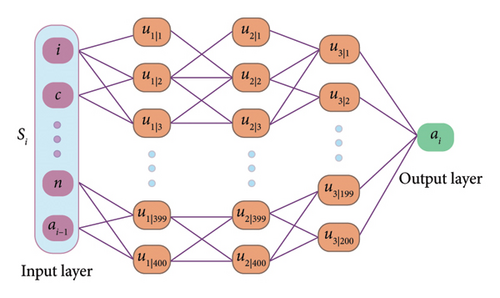
As shown in Figure 1, the input layer contains nine neurons, and the current state S_i is adopted as the input vector of the actor network. The output of the actor network is the pruning ratio of the fault diagnosis network, which is signified as a_i. The actor network in this paper contains three hidden layers, and the numbers of the neurons in three hidden layers are 400, 400, and 200, respectively.

The loss function of the actor network can be represented as the following equation:

$$\begin{array}{}\text{Los}{\text{s}}_{\text{Actor}}=-Q_w\left(S_i,a_i\right)=-Q_w\left(S_i,{\mu }_{\theta }\left(S_i\right)\right),\end{array}$$ ()

where Loss_Actor represents the loss of the actor network and Q_w(S_i, a_i) represents the output of the critic network, which represents the expected value of the actor a_i under the state S_i. μ_θ(S_i) represents the output of the actor network under the parameter matrix θ, as shown in the following equation:

$$\begin{array}{}{a}_i={\mu }_{\theta }\left(S_i\right).\end{array}$$ ()

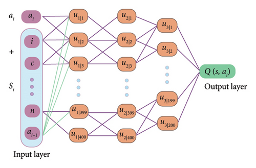
The critic network is responsible for predicting the value of the actor a_i. Unlike the actor network, the critic network takes the pruning ratio and the state as the input vector. The output of the critic network is the expected value of the actor a_i. The basic structure of the critic network is a multilayer fully connected network, which is identical to the actor network. The structure of the critic network is illustrated in Figure 2.

The proposed compression method prunes the 1-DCNN for the fault diagnosis based on the reinforcement learning method. The environment for the NP should include the network for the fault diagnosis, the dataset, and the reward function.

After the environment executes the pruning action and returns the reward r_i, we proceed to redefine the function of the reward as depicted in the following equation:

$$\begin{array}{}{r}_i=\alpha \mathrm{\ast }\text{acc}\_\text{loss}+\beta \mathrm{\ast }\text{rate}\_\text{FLOPs}+\gamma \mathrm{\ast }\text{rate}\_\text{parameters},\end{array}$$ ()

where acc_loss represents the loss of the network’s accuracy after each pruning action, rate_FLOPs represents the compression ratio of the FLOPs of the entire network, rate_parameters represents the compression ratio of the parameters of the entire network, and α, β, and γ are the adjustment parameters.

The gradient descent strategy is employed to update the parameters of both networks using the TD-error. The output of the critic network is considered as the expected value Q_w(S_i, a_i) of the actor a_i under the state S_i. $Q_{w^{`}}\left(S_{i+1},a_{i+1}\right)$ represents the output of the target critic network. The real-time reward of the actor a_i under the state S_i is denoted as r. The expected value is defined as shown in the following equation:

$$\begin{array}{}{Q}_{\text{target}}=r+\gamma Q_{\stackrel{`}{w}}\left(S_{i+1},a_{i+1}\right),\end{array}$$ ()

where γ is the update ratio of the critic network.

By subtracting Q_target from Q_w(S_i, a_i), we obtain the mean square as the loss function of the critic network. Therefore, the loss function of the critic network is defined as shown in the following equation:

$$\begin{array}{}\text{Los}{\text{s}}_{\text{Critic}}=\text{MSE}\left(Q_w\left(S_i,a_i\right),r+\gamma Q_{w^{`}}\left(S_{i+1},a_{i+1}\right)\right).\end{array}$$ ()

The DDPG algorithm is employed to optimize the pruning process. The training process, which is based on the NP process, is shown in Table 1.

Table 1. The pruning process based on the DDPG.

Algorithm 1: Pruning the kernels in each layer of the 1DCNN using the DDPG algorithm
Randomly initialize the actor network μ(S|θμ) and the critic network Q(S, a|θQ) with the weights θμ and θQ
Initialize the reply buffer M
For episode = 1, N do
Initialize a random process Π for the action exploration
Receive the initial observation state (S1)
For t = 1 to T do
Select an action(at = μ(St|θμ) + Πt) according to the current policy and the exploration noise
Execute the action (at) and observe the reward (rt), observe the new state (St+1)
Store the transition (St, at, rt, St+1) in the buffer M
Sample a random mini-batch of N transitions (Si, ai, ri, Si+1) from the buffer M
Set $Q_{\text{target}}=r+\gamma Q^{\prime }\left(S_{i+1},\mu \prime \left(S_{i+1}\left|{\theta }^{{\mu }^{\prime }}\right.\right)\left|{\theta }^{Q^{\prime }}\right.\right)$
Update the parameters of the critic network by minimizing the loss:
LossCritic = MSE(Qw(Si, ai), r + γQ′(Si+1, ai+1))
Update the parameters of the actor network with the loss function of:
LossActor = −Qw(Si, ai) = −Qw(Si, μθ(Si))
Update the parameters of the target networks with the function of:
${\theta }^{Q^{\prime }}⟵\tau {\theta }^Q+\left(1-\tau \right){\theta }^{Q^{\prime }},$
${\theta }^{{\mu }^{\prime }}⟵\tau {\theta }^{\mu }+\left(1-\tau \right){\theta }^{{\mu }^{\prime }}.$
End for
End for

2.2. NP

The NP methods can be broadly categorized into two main types: structured pruning and unstructured pruning [50]. In the unstructured pruning method, less important neurons or parameters in the network are removed. Consequently, the connections between the pruned neurons and other neurons are disregarded during computation. However, accelerating the pruned network after the unstructured pruning process is challenging for existing typical hardware architectures. The deployment of the pruned network with fine-grained pruning methods necessitates specialized hardware platforms [51]. This requirement poses a hindrance to the widespread application of such pruning algorithms at a large scale.

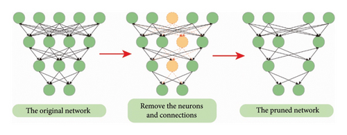
Structured pruning typically involves pruning at the filter or entire network layer, and the next feature maps undergo corresponding changes, but the overall structure of the model remains intact. As a result, it can still be accelerated using GPUs or other hardware, making it known as structured pruning. The deployment of the pruned network using this method does not rely on specialized hardware platforms. This type of pruning method offers good versatility. Therefore, for the 1-DCNN, the compression method based on pruning convolutional kernels and neurons in FL is adopted. This article primarily focuses on pruning convolutional kernels in CL and neurons in FL.

For the one-dimensional CL, we perform pruning on the number of convolutional kernels. The size of the convolutional kernel is denoted as n × c × k, where n represents the number of convolutional kernels, c signifies the number of channels in each convolutional kernel, and k indicates the length of the convolutional kernel weight in each channel. To determine the importance of each convolutional kernel, we calculate the L1 norm of its weight. The importance of ith convolutional kernel can be calculated as follows:

$$\begin{array}{}{\text{importance}}_i={\displaystyle \sum }_c{\displaystyle \sum }_k\left|w_{c,k}\right|,\end{array}$$ ()

where i is the index of the convolutional kernel in each layer.

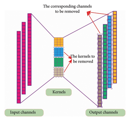
The larger the value of the L1 norm, the greater the importance of the convolutional kernel. For the pruning process, we remove the convolutional kernels with the less importance value. When the number of the convolutional kernels is changed, the number of the output channels accordingly. For the number of the output channels, it must keep the same as the convolutional kernels. The schematic diagram of the convolutional kernel pruning process is shown in Figure 3.

For the FL, we take the neuron as the object to be pruned. The corresponding forward and backward connections of the pruned neurons must also be eliminated. The schematic diagram in Figure 4 illustrates the process of neuron pruning for the FL. The size of the weight matrix can be represented as m × n, where m is the number of output neurons and n is the number of input neurons. The importance of the neurons is determined by the L1 norm. Therefore, the importance of the jth neuron can be calculated as follows:

$$\begin{array}{}{\text{importance}}_j={\displaystyle \sum }_{k=1}^n\left|W_{j,k}\right|.\end{array}$$ ()

2.3. K-D

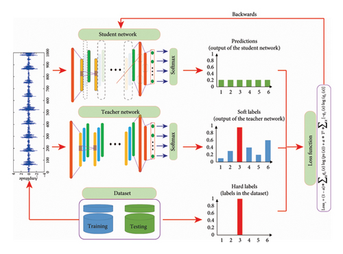
After pruning the convolutional kernels or neurons in the network, the performance of the network will be somewhat affected. This is due to the alterations in the structure and parameters of the network resulting from the pruning process. To enhance the performance of the pruned network, the K-D process is introduced to fine-tune the parameters of the pruned network in each iteration. The fundamental process of K-D is illustrated in Figure 5.

To carry out the K-D process, the following steps are followed. Firstly, the original network that is to be pruned is trained, and the trained model is saved as the teacher network. The pruned network obtained in each pruning iteration is considered as the student network. During the training of the student network, the same training samples are fed to both the teacher network and the student network. The outputs of the teacher network serve as the soft labels, while the labels in the training dataset are considered as the hard labels. Using the outputs of the student network, the soft labels, and the hard labels, the loss function of the student network is reconstructed. The parameters of the student network are then optimized using the back-propagation algorithm. The loss function of the student network is defined as the following equation:

$$\begin{array}{}\text{Los}{\text{s}}_s=\left(1-\alpha \right)\mathrm{\ast }{\displaystyle \sum }_x{q}_s\left(x\right)\log \left(p_s\left(x\right)\right)+\alpha \mathrm{\ast }{T}^2\mathrm{\ast }{\displaystyle \sum }_x\left[-q_T\left(x\right)\log \left(q_s\left(x\right)\right)\right],\end{array}$$ ()

where α represents an adjustment factor, q_s(x) denotes the outputs of the student network, p_s(x) represents the distribution of the hard label, q_T(x) signifies the output of the teacher network, and T represents the hyperparameter of the distillation temperature.

2.4. The Calculation Method of the FLOPs and the Amount of the Parameters

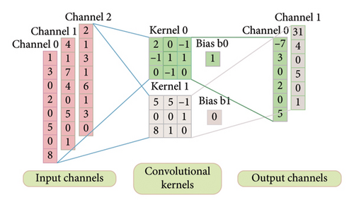
When deploying the network on an embedded hardware platform, the primary considerations are the storage requirements and the number of FLOPs of the network. During inference computation on the hardware platform, a smaller size of network parameters results in less memory space being needed. Similarly, a smaller number of FLOPs leads to faster inference speed and better real-time performance. In the field of neural network compression, the abovementioned two metrics are commonly used to evaluate the compression algorithm. Therefore, this section provides a brief introduction to the calculation method to determine the number of parameters and FLOPs in the network. The basic structure of the one-dimensional layer is illustrated in Figure 6.

As shown in Figure 6, the main parts of the one-dimensional CL are input vectors, convolutional kernels, and output vectors. Therefore, the number of the parameters contained in a one-dimensional CL can be calculated as follows:

$$\begin{array}{}\text{Parameters}\_\text{CL}=c\mathrm{\ast }n+k\mathrm{\ast }c\mathrm{\ast }l+k+k\mathrm{\ast }m+2p\mathrm{\ast }c,\end{array}$$ ()

where Parameters_CL represents the number of parameters in the one-dimensional layer, c denotes the number of input channels, n signifies the length of the input channel, k represents the number of convolutional kernels, m denotes the length of the output channel, and p represents the number of padding data.

When the one-dimensional CL performs forward inference, the number of FLOPs can be calculated using equation (11):

$$\begin{array}{}\text{FLOPs}\_\text{CL}=m\mathrm{\ast }k\mathrm{\ast }c\mathrm{\ast }l+k,\end{array}$$ ()

where FLOPs_CL is the FLOPs of the one-dimensional CL.

For the FL, the number of the parameters Parameters_FC contained in a FL can be calculated as (12) follows:

$$\begin{array}{}\text{Parameters}\_\text{FC}=n+2m+m·n.\end{array}$$ ()

The FLOPs of the FL FLOPs_FC can be calculated as follows:

$$\begin{array}{}\text{FLOPs}\_\text{FC}=m\times n+m,\end{array}$$ ()

where n is the number of the input neurons and m is the number of the output neurons.

3. Methodology

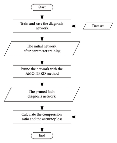
To address the issue of poor real-time performance in deep neural networks, the process of NP and K-D is employed to compress the pretrained network. To minimize manual effort during the compression process, the DDPG algorithm is utilized to automate the pruning operation. The network, dataset, and pruning process together form the environment. The information of each layer (kernels, size, and padding) is treated as the state strategy that is adopted to enhance the overall compression rate of the network. After each round of pruning, the K-D process is the subsequent pruning round. The flowchart of the proposed method is depicted in Figure 7.

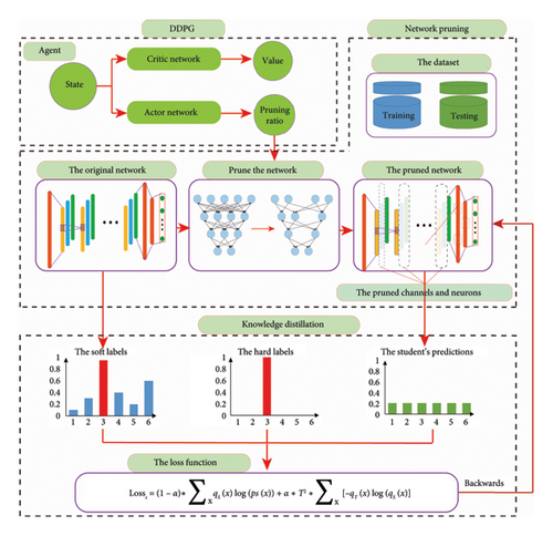
The proposed method can be summarized as follows:

Firstly, the agent is built, consisting of an action network and a critic network. The action network takes the state information of the network in the pruning environment as input and outputs the pruning ratio for each layer. The critic network evaluates the value of the pruning ratio, taking the state information and pruning ratio as inputs. Typically, both the actor and critic networks can be implemented using a multilayer fully connected network.

Secondly, the network is pruned based on the given pruning ratio. Specifically, the focus is on pruning the commonly used convolutional neural network for bearing fault diagnosis. Structured pruning is adopted to CL, and pruning is performed in the dimension of convolutional kernels, while for FL, pruning is performed in the neuron dimension.

Thirdly, the pruned network is fine-tuned using the K-D method. This step aims to further optimize the parameters of the pruned network and compensate for the loss of accuracy caused by the pruning process. The original network serves as the teacher network, with its outputs used as soft labels. The pruned network in each iteration is treated as the student network. The one-hot labels in the dataset are considered hard labels. The loss function of the student network is reconstructed based on the hard labels, soft labels, and outputs of the student network. Back-propagation is then performed to optimize the student network.

Finally, the pruning and fine-tuning process is conducted based on the DDPG algorithm. The entire process is treated as a Markov process, and an environment is built to encompass network pruning, fine-tuning, accuracy testing, and network analysis. By considering factors such as accuracy and parameter scale of the pruned network, a value function is established to guide the NP process. Using this value function and DDPG, the optimal pruning strategy for each iteration can be determined. The pruned network is fine-tuned using the K-D process, and this network becomes the original network for the next iteration. The pruning and fine-tuning process is repeated, resulting in a balanced parameter scale and performance.

4. Experiment Results and Discussion

To validate the effectiveness of the proposed AMC-NPKD method, experiments are conducted on two different test benches with distinct structures. The detailed experimental flowchart is in Figure 8. The experiments are performed using JetBrains PyCharm with the 2019® community edition as the software environment. The PyTorch deep learning framework is utilized. The experimental setup consists of an i3-8100 CPU, a GTX3060 GPU, 32 GB of memory, and a 2 TB hard drive.

4.1. Results on the CWRU Dataset

4.1.1. The Dataset Description

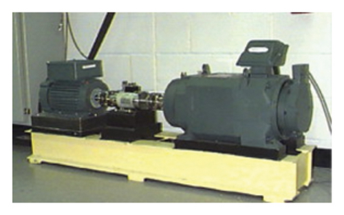
In this experiment, the dataset from the CWRU Bearing Data Center [52] is utilized for testing. The device used to generate the bearing fault dataset is depicted in Figure 9. The dataset comprises monitoring data from four bearing states: the health state, the inner race fault state, the ball fault state and the outer race fault state. The inner ring fault in the experiment was collected during tests conducted on a 2-hp Reliance electric motor. Vibration data were recorded for motor loads ranging from 0 to 3.

For the experiment, monitoring data with different health states and running speeds were utilized. The details of the data used in this experiment are presented in Table 2. There are 8 types of monitoring data used for network training and testing, with labels ranging from 0 to 7. Each sample has a length of 2048. For each type of monitoring data, 4000 samples are used for training, and 1000 samples are used for testing in the K-D process. In total, the dataset consists of 40,000 samples, enabling the compression process for network training and testing.

Table 2. The CWRU-bearing dataset adopted in the experiment.

Running speed (rpm)	Health	Inner race fault	Ball fault	Outer race fault
1797	97.mat	105.mat	118.mat	130.mat
1730	100.mat	108.mat	121.mat	133.mat

4.1.2. The Structure of the Network to be Pruned

In the field of the bearing fault diagnosis, the vibration signal is commonly used for the monitoring task. In order to facilitate the process of the fault diagnosis, the 1-DCNN is adopted to directly process the vibration signals in the time domain. Therefore, this experiment mainly prunes the 1-DCNN, which was proposed in our previous work [31], to verify the effectiveness of the proposed AMC-NPKD method. The structure and the details of the original network are shown in Table 3.

Table 3. The details of the original network to be pruned.

Layers	Kernel size/stride	Kernel number	Output size	Padding
CL1	64 × 1/8 × 1	16	256 × 16	Yes
PL1	2 × 1/2 × 1	16	128 × 16	No
CL2	3 × 1/1 × 1	32	128 × 32	Yes
PL2	2 × 1/2 × 1	32	64 × 32	No
CL3	3 × 1/1 × 1	64	64 × 64	Yes
PL3	2 × 1/2 × 1	64	32 × 64	No
CL4	3 × 1/1 × 1	64	32 × 64	Yes
PL4	2 × 1/2 × 1	64	16 × 64	No
CL5	3 × 1/1 × 1	64	16 × 64	Yes
PL5	2 × 1/2 × 1	64	8 × 64	No
FL1	/	/	512 × 1
FL2	/	/	200 × 1
Output	/	/	8

From Table 3, it is evident that the proposed WDCNN consists of 5 CL and 2 FL. The length of the convolutional kernels in the first layer is 64, while the numbers of the neuron in the two FL are 512 and 200, respectively. Based on calculations of the number of parameters and FLOPs, the WDCNN mentioned above has 273.7 k parameters and 1648.6 k FLOPs.

4.1.3. The Results on the CWRU Dataset

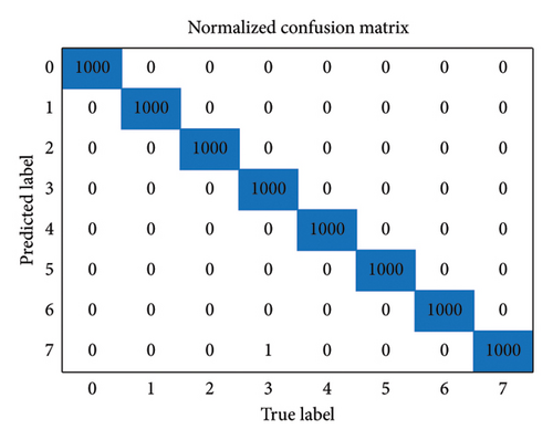
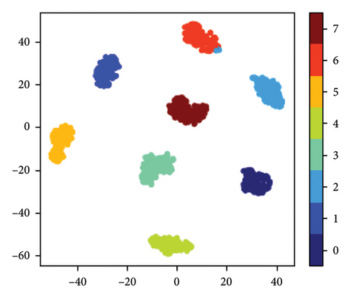
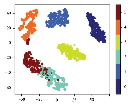
In each iteration of the DDPG training process, the specifications and experimental parameters in the experiment are set as in Table 4. The pruning results for each iteration throughout the entire pruning process are presented in Table 5 and Figure 10. The confusion matrices of the original network and the pruned network are displayed in Figure 11. The results of feature visualization for the two networks are shown in Figure 12.

Table 4. The specifications and experimental parameters in the experiment.

Name	Training times for DDPG	Maximum pruning ratio for each layer	Training epoch of K-D	Learning rate	Batch size
Value	1000	0.99	1000	1.0e − 4	40

Table 5. The results of pruning the WDCNN based on the CWRU bearing dataset.

Iteration number	The shape of the pruned network	Parameters (K)	FLOPs (K)	Accuracy (%)	Compression ratio (%)
0	[16, 32, 64, 64, 64, 512, 200, 8]	273.7	1648.6	100	0
1	[12, 22, 51, 46, 47,376, 88, 8]	110.8	909.6	100	44.83
2	[5, 9, 22, 14, 12, 96, 40, 8]	22.1	183.3	99.96	88.88
3	[3, 6, 17, 10, 11, 88, 17, 8]	13.0	100.5	99.87	93.90
4	[1, 5, 4, 5, 10, 80, 10, 8]	7.1	28.2	99.81	98.29
5	[1, 5, 4, 5, 10, 80, 10, 8]	7.1	28.2	99.81	98.29
6	[1, 5, 4, 5, 10, 80, 10, 8]	7.1	28.2	99.81	98.29
7	[1, 5, 4, 5, 10, 80, 10, 8]	7.1	28.2	99.81	98.29
8	[1, 5, 4, 5, 10, 80, 10, 8]	7.1	28.2	99.81	98.29
9	[1, 5, 4, 5, 10, 80, 10, 8]	7.1	28.2	99.81	98.29
10	[1, 5, 4, 5, 10, 80, 10, 8]	7.1	28.2	99.81	98.29

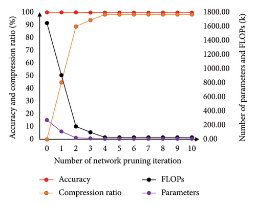
From Table 4 and Figure 10, it can be observed that the accuracy of the original network is 100%, while the pruned network achieves an accuracy of 99.81%. This indicates that there is minimal loss in accuracy after the pruning process. The FLOPs of the original network and the pruned network are 1648.6.2 and 28.2 K, respectively, resulting in a compression ratio of 98.29%. The number of parameters in the original network is 273.7 K, while the pruned network has 7.1 K parameters, resulting in a compression ratio of 97.41%. These results demonstrate that the proposed AMC-NPKD method can significantly compress the size of the neural network while maintaining a high level of accuracy.

In Table 4, it can be observed that the pruning ratio varies in each iteration, as well as across different layers. This is because the actor network provides the pruning ratio based on the real-time state. By optimizing the parameters of the actor network using the DDPG algorithm, the actor network outputs the best pruning ratio according to the current state.

From Figures 11 and 12, it can be concluded that the classification performance and robustness of the pruned network have not been significantly affected. The confusion matrices show that the classification performance for each sample type remains nearly the same after the pruning process. The robustness of the network is also maintained, as the distance between the extracted features is not shortened. Despite the significant compression achieved by the AMC-NPKD method, the performance of the pruned network remains largely unaffected. This further validates the effectiveness of the proposed AMC-NPKD method.

4.2. Results on HIT-SM Datasets

4.2.1. The Dataset Description

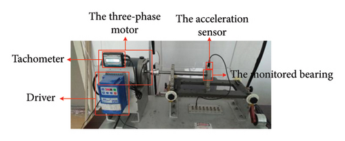
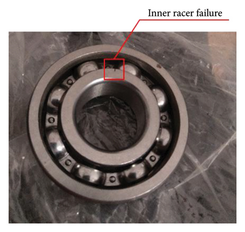
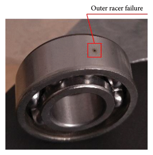
To further validate the effectiveness of the proposed AMC-NPKD method, an experiment is conducted using the HIT-SM bearing datasets [53]. The composition of the equipment used in the experiment is depicted in Figure 13. The bearing under test is a deep groove ball bearing with a model number of 6205. Three states of the bearings are tested: the healthy state, the inner ring failure state (as shown in Figure 14(a)), and the outer ring failure state (as shown in Figure 14(b)). The fault area is created using electrical discharge machining (EDM). The dataset is collected at speeds of 900 and 1200 RPM, with a sampling frequency of 51.2 kHz.

To evaluate the classification performance of the networks, six types of monitoring data are utilized. The dataset consists of three states of bearings under different speeds. The specifics of the dataset are presented in Table 6. For each type of sample, there are a total of 10,000 samples. Among these, 8000 samples are used for training, while the remaining 2000 samples are used for testing.

Table 6. The number of samples adopted in the experiment based on the HIT-SM bearing dataset.

Running speed (rpm)	Health	Inner race fault	Outer race fault
900	10,000	10,000	10,000
1200	10,000	10,000	10,000

4.2.2. The Results on the HIT-SM Bearing Dataset

In this experiment, the WDCNN is also used as the original network to be pruned. The details of the WDCNN adopted in this experiment are similar to those in Table 2, with the only difference being that the output layer of the WDCNN used in this experiment contains 6 neurons. This is because the dataset used in this experiment consists of only 6 types of samples. The hyperparameters used in this experiment remain the same as those in the previous experiment.

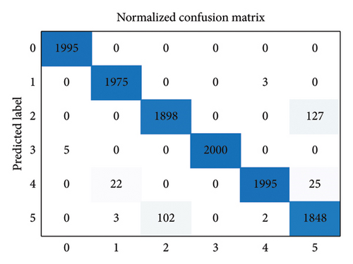
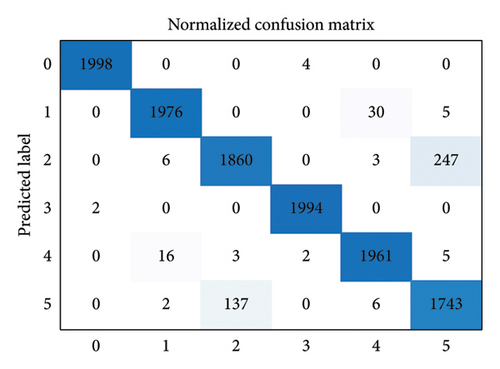
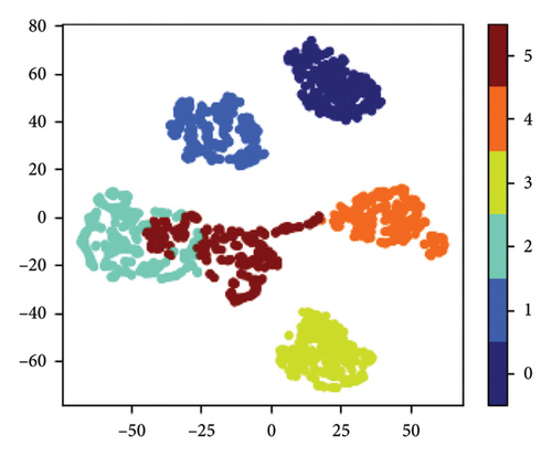
The structure of the network to be pruned in this experiment is the same as before, with the only difference being that the output layer now has six neurons to accommodate the six types of samples in the dataset. The remaining hyperparameters remain unchanged from the previous experiment. The pruning results for each iteration throughout the entire pruning process are presented in Table 7 and Figure 15. The confusion matrices of the original network and the pruned network are displayed in Figure 16. The results of feature visualization for the two networks are shown in Figure 17.

Table 7. The results of pruning the WDCNN based on the HIT-SM bearing dataset.

Iteration number	The shape of the pruned network	Parameters (K)	FLOPs (K)	Accuracy (%)	Compression ratio (%)
0	[16, 32, 64, 64, 64, 512, 200, 6]	273.3	1648.2	97.59	0
1	[9, 14, 26, 18, 16, 128, 42, 6]	30.9	335.6	97.48	79.64
2	[5, 8, 14, 10, 7, 56, 21, 6]	13.4	138.1	96.17	91.62
3	[2, 5, 4, 14, 6, 48, 15, 6]	8.3	51.4	96.10	96.88
4	[2, 5, 4, 14, 6, 48, 15, 6]	8.3	51.4	96.10	96.88
5	[2, 5, 4, 14, 6, 48, 15, 6]	8.3	51.4	96.10	96.88
6	[2, 5, 4, 14, 6, 48, 15, 6]	8.3	51.4	96.10	96.88
7	[2, 5, 4, 14, 6, 48, 15, 6]	8.3	51.4	96.10	96.88
8	[2, 5, 4, 14, 6, 48, 15, 6]	8.3	51.4	96.10	96.88
9	[2, 5, 4, 14, 6, 48, 15, 6]	8.3	51.4	96.10	96.88
10	[2, 5, 4, 14, 6, 48, 15, 6]	8.3	51.4	96.10	96.88

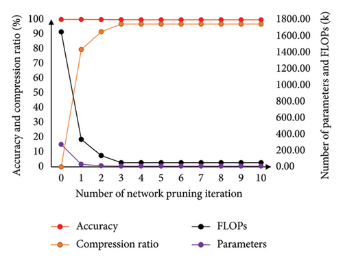
From Table 7 and Figure 15, it can be observed that the accuracy of the original network is 97.59%, while the pruned network achieves an accuracy of 96.10%. This indicates that the loss in accuracy after the pruning process is only 1.49%. The FLOPs of the original network and the pruned network are 1648.2 and 51.4 K, respectively, resulting in a compression ratio of 96.88%. The number of parameters in the original network is 273.3 K, while the pruned network has 8.3 K parameters, resulting in a compression ratio of 96.96%. The accuracy of the pruned network remains nearly unchanged compared to the original network. The proposed AMC-NPKD method effectively compresses the size of the neural network using the home-made dataset. These experimental results further demonstrate the effectiveness and generalization of the proposed AMC-NPKD method.

From Figures 16 and 17, it can be concluded that the classification performance and robustness of the pruned network have not been significantly affected using the home-made dataset. The robustness of the network is also maintained, as the distance between the extracted features remains unchanged. Despite the significant compression achieved by the AMC-NPKD method, the performance of the pruned network remains largely unaffected. This further validates the effectiveness of the proposed AMC-NPKD method.

4.4. Ablation Study

The effectiveness of the proposed method can be aforementioned cases. The efficiency of the proposed method is achieved through the combination of several improvements, including the iterative pruning process and the fine-tuning step based on K-D. The effects of each improvement are analyzed separately in this section.

4.4.1. The Influence of the Iterative Pruning Process

He et al. proposed the AutoML method for automatic network compression [49]. In this study, we enhance the AutoML method by introducing an iterative pruning process. This iterative pruning step allows for a higher pruning ratio to be achieved for the network. To evaluate the effectiveness of the iterative pruning step, comparative experiments are conducted in this section. The accuracy and compression ratios of the AutoML method and the proposed AMC-NPKD method are presented in Table 9. The compression ratios and details of the pruned networks using both methods are illustrated in Figure 18.

Table 9. The results of the two methods to prune the WDCNN with the HIT-SM bearing dataset.

Method	Accuracy (%)	Parameters (K)	FLOPs (K)	Compression rate (%)
WDCNN (original network)	97.59	169.2	1648.2	—
AutoML	93.07	50.8	787.7	52.21
AMC-NPKD	96.10	8.3	51.4	96.88

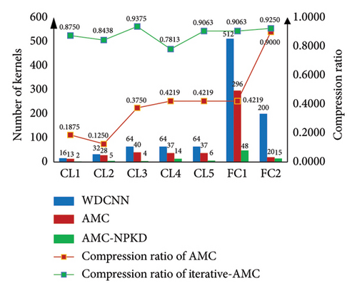
From Table 9 and Figure 18, it is evident that the accuracy of the pruned network using the AutoML method is 93.07%, with a loss of 3.29% compared to the original network. However, the loss in accuracy for the pruned network using the proposed AMC-NPKD method is only 1.49%. In terms of the network compression ratio, the pruning ratios for the original network are 52.21% and 96.88% for AutoML and AMC-NPKD, respectively. Regarding the scale of the pruned networks, the number of parameters in the pruned network obtained with AMC-NPKD is only 0.163 times that of AutoML. Similarly, the FLOPs of the pruned network with AMC-NPKD is only 0.065 times that of AutoML. Through the ablation study and result analysis, it is evident that by incorporating the iterative pruning strategy, the proposed AMC-NPKD method achieves a higher NP ratio.

The proposed AMP-NPKD method can repeatedly prune and train the compressed neural network through the iterative pruning strategy. After a single round of NP, the parameters of the new neural network obtained after pruning are optimized and allocated, so as to maximize the performance potential of the neural network obtained after pruning. Finally, a lightweight neural network with a more streamlined structure can be obtained. Therefore, a higher compression ratio of the neural network can be addressed.

4.4.2. The Influence of the Fine-Tuning Step With the K-D Method

In the proposed AMC-NPKD method, a fine-tuning step based on the K-D process is implemented after each pruning iteration. When the pretrained network is pruned, the performance of the pruned network may be affected due to the reduction in parameters and structures. Additionally, the parameter distribution of the pruned network may not be optimally suited for the current network structure. To further enhance the performance of the pruned network, the K-D process is employed to fine-tune the pruned network after each iteration. The fine-tuned pruned network then serves as the original network for the subsequent pruning iteration. To evaluate the impact of the K-D fine-tuning process, an ablation experiment is conducted. The comparative method used is an iterative AutoML method, where a fine-tuning step is performed after each pruning iteration using the normal network training process without the K-D process. The results of the original WDCNN, the comparative method, and the proposed AMC-NPKD method are presented in Table 10 and Figure 19.

Table 10. The results of the two methods to prune the WDCNN with the HIT-SM bearing dataset.

Method	Accuracy (%)	Parameters (K)	FLOPs (K)	Compression rate (%)
WDCNN (original network)	97.59	273.3	1648.2	—
The comparative method	96.06	8.8	53.8	96.74
AMC-NPKD	96.10	8.3	51.4	96.88

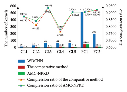
From Table 10 and Figure 19, the results demonstrate that the proposed AMC-NPKD method achieves a higher compression ratio and classification accuracy compared to the comparative method. The final compression rates of the pruned networks using the two methods are 96.74% and 96.88%, respectively. The accuracies of the pruned networks using the two methods are 96.06% and 96.10%, respectively.

The proposed method, which incorporates the K-D process in the fine-tuning steps, outperforms the iterative AutoML method without the K-D process. This is because the K-D process can enhance the performance of the pruned network. Compared to the normal network training process, the K-D process further explores the potential performance of the small pruned network. As a result, the proposed AMC-NPKD method achieves a higher network compression ratio.

5. Conclusion

In order to solve the problem of a large parameter scale and large consumption of hardware computing resources in the current fault diagnosis neural network model, this paper proposes an AMC-NPKD method to achieve deep compression and optimization of the fault diagnosis neural network. Based on the AutoML method, the proposed AMC-NPKD method introduces the iterative pruning strategy and the K-D process to realize cyclic pruning and parameter optimization for the compressed neural network model and finally obtains a higher network compression ratio. Experimental results show that the proposed AMC-NPKD method compresses the computational amount of the WDCNN network by more than 96% and the compression rate of parameters by more than 95%. The comparative experimental results show that the AMC-NPKD method also achieves significant advantages compared with the current typical lightweight neural network model design and compression methods. The AMC-NPKD method proposed in this paper is a kind of the network compression algorithm with strong generality, which is not only suitable for bearing fault diagnosis research but also is expected to have good performance in speech recognition, image recognition, and other research fields. The further research can be carried out in this field in the follow-up work.

The proposed AMC-NPKD method is a structured pruning method, where the entire convolution kernel or neuron is pruned. In future studies, we plan to explore network pruning in smaller dimensions, such as the channel of the convolutional kernel.

Conflicts of Interest

The authors declare no conflicts of interest.

Funding

This research was supported by the Aviation Key Laboratory of Science and Technology on Aero Electromechanical System Integration, Nanjing Engineering Institute of Aircraft Systems, AVIC.