Research on Predicting Mine Earthquakes Based on Deep Learning Time-Series Methods
Abstract
As the depth and intensity of coal mining in China continue to increase, the frequency and intensity of coal mine earthquakes are also rising exponentially. The occurrence of strong mine earthquakes may result in dynamic disasters, such as impact ground pressure, which pose a significant threat to the lives and properties of individuals residing in mining regions. To more accurately monitor and predict mine earthquakes and thereby reduce the potential risk they pose, this paper presents a study on the inversion and localization of seismic sources of mine earthquakes and a study on the prediction of mine earthquakes based on the deep learning method. The latter is set in the context of the Dongtan coal mine. The principal findings are as follows: The Informer time-series prediction model employs historical data on daily maximum energy mine earthquakes to predict the source location coordinates of possible future daily maximum energy mine earthquakes. The Informer time-series prediction model demonstrates superior performance in the task of mine earthquake prediction, outperforming the prediction of the location of the mine earthquakes’ source coordinates than the prediction of the energy magnitude of the mine earthquakes.
1. Introduction
Mine earthquake is induced by mining disturbance. It is a response of coal and rock mass to regional or local stress adjustment in the process of coal mining. Mine earthquake is usually accompanied by energy release and vibration. The essential reason is that there is a high stress or high stress difference in coal and rock mass [1, 2]. In recent years, the frequent occurrence of large-energy mine earthquakes has led to obvious ground vibration, which has also seriously affected the normal life of residents near the mining area, and the social impact is bad [3].
The connotation of mine earthquake risk prediction is to use the theory or data method to analyze the information law before the occurrence of a mine earthquake and construct the appropriate prediction and early warning index to warn the mine earthquake [4]. Yin et al. found that there is an inextricable relationship between mine earthquakes and natural earthquakes, and their results show that mines where mine earthquakes occur in the planar distribution also belong to the natural earthquake-prone zones, and almost all of them are distributed in seismic zones with strong tectonic activity [5]. There is a great similarity between the field of earthquake prediction and the field of mine earthquake prediction [6]. Therefore, many scholars have applied the method of earthquake prediction to mine earthquake prediction. Les used the mean minimum distance clustering (MMD) to determine the number of seismic event clusters, hierarchical clustering, and K-means clustering to verify the identification results, identified 31 independent seismic event clusters, and pointed out possible dangerous areas. Dense microseismic activity may indicate the occurrence of high-energy microseismic events [7]. Li et al. determined the maximum dynamic response range of impact vibration damage according to the energy attenuation law of impact vibration in geotechnical media and proposed a zonal monitoring method for mine earthquake precursors [8]. The results of their study showed that after the occurrence of earthquake ground pressure, the energy of the mine earthquake and the number of mine earthquakes decreased rapidly because of the release of a large amount of elastic potential energy gathered in the coal rock body by the earthquake ground pressure. The mine earthquake zoning monitoring method quickly and accurately reflects the trend of mine earthquake changes in the mining area and serves as an early warning for other dynamic disasters. Zhou applied the latest results of nonlinear dynamics, which is mainly based on chaos theory, to conduct a more comprehensive and systematic research on the chaotic nature and nonlinear prediction theory in the process of mine earthquake gestation and evolution [9]. Li et al. analyzed data acquired during strong mine earthquakes with seismological methods and wavelet tools based on field observations from a network of high-density digital seismic and tidal deformation stations at the Mesoscale Seismic Experimental Site [10]. Seismological anomalies such as credible b-value, n-value, frequency, and fixed-point tidal deformation precursor anomalies are found to exist in the pre-earthquake short-critical phase, and the methods of extracting anomalous information and predicting the short-critical phase of strong mine earthquakes are discussed.
With the rise of artificial intelligence big data, various algorithms such as machine learning and deep learning have also been applied to the fields of landslide deformation prediction and mine earthquake prediction. Li et al. proposed a deep learning–based framework for modeling and predicting the reservoir landslide deformation displacement in the Three Gorges Reservoir. In his study, a data-driven framework using deep belief network and control chart has been introduced to explore the temporal patterns of displacement and potential of identifying seasonal faster displacement, and comparative analysis using state-of-the-art algorithms, including k-nearest neighbor, random forest, neural network, support vector machine (SVM), and extreme learning machine, were performed to validate the efficiency and accuracy of the deep belief network [11]. Accurate segmentation and measurement of loess landslides is crucial for documenting their occurrence and extent and investigating the distribution, types, and patterns of slope failures. Li et al. proposed a novel data-driven framework for the segmentation and measurement of loess landslides from remote sensing satellite images. The developed framework was benchmarked against a set of state-of-the-art deep-learning semantic segmentation algorithms. Computational results demonstrate that the proposed approach outperforms other state-of-the-art algorithms in terms of the measurement metrics related to the overall segmentation accuracy and boundary distances. It was shown that the proposed approach achieved comparable reliability, better segmentation quality, and better predicted boundary for loess landslides than the state-of-the-art algorithms [12]. Nustes Andrade and van der Baan applied convolutional neural network (CNN) to t predict microseismic clouds in hydraulic fracturing, and his results showed that CNN outperforms the prediction quality of physical-based model, but the prediction ability is slightly reduced. However, adding physical constraints to the prediction model can improve the prediction of CNN [13]. Wang et al. collected a large amount of microseismic data from the panel of Shoushan Mine of the Pingdingshan Coal Group and filtered the data. Then, a microseismic data prediction model was constructed based on the three-dimensional coordinates of the underground space by using genetic programming (GP), and prediction formulas were established for the magnitude and the energy through the GP, and real-time evolutions of each parameter were obtained of the optimal individual [14]. Pei et al. developed a time series prediction model for microseismic energy levels based on a one-dimensional CNN and used a hybrid sampling method to realize the energy levels of the previous 10 microseismic events as inputs to predict the energy level of the next microseismic event [15]. Lv and Pan used the ARIMA seasonal model to predict future microseismic events and introduced a threshold autoregressive model to improve prediction accuracy when the period of high-energy microseismic events is unstable, so as to achieve short-term prediction with high accuracy [16]. Cao et al. integrated the explicit features of physical indicators with data-driven implicit features and used deep learning CNN to process the fusion features to obtain the classification results. In engineering practice, the prediction results of the next day, 2 days and 3 days were obtained, and the accuracy rate was high [17]. Vardaan et al. proposed a model based on long short-term memory (LSTM) recurrent neural network to predict earthquake trends and compared it with feedforward neural network (FNN). The results show that the LSTM model can predict data such as time, location and magnitude of earthquakes, which is significantly better than the FNN method [18]. To understand Jishishan earthquake’s seismogenesis, Dong and Yang employed state-of-the-art full-waveform tomography to obtain high-resolution, multiparameter seismic models of the crust surrounding the epicenter [19]. Ebrahimi-Mamaghani et al. has numerically and analytically investigated the dynamics of underwater movable porous functional gradient (FG) micro-sized beams with integrated piezoelectric layers. In addition, the efficiency and accuracy of the SVM technique for microbeam vibration prediction are evaluated [20]. Li et al. focused on the Haiyuan-Liupanshan region, aiming to obtain source depth profile images of the study area by detecting microseismic catalogs, and to calculate b-value parameter plane scans based on microseismic results. Ultimately, by combining the source depth profiles and b-value plane scan images, an analysis was conducted to determine the distribution relationship between high-stress zones, tectonics, and earthquakes in the region [21]. An efficient and universal large-scale seismic implicit analysis procedure incorporating GPU acceleration for the preconditioned conjugate gradient algorithm and Ritz vector method is systematically proposed by Li et al. A global method for SSSI nonlinear analysis was improved for efficiency on the surface elemental form of viscous-spring artificial boundary, batch computation of seismic equivalent forces, and viscoelastic constitution of soils. A refined-modeled reactor building was investigated under typical scenarios to reveal the rules [22]. Zhang et al. presented a comprehensive analysis of the influence of different UHPC replacement heights and the incorporation of CFRP plates on the hysteretic properties of beams under cyclic loading conditions. Their findings introduce new insights into the structural dynamics of composite beams [23]. Wang et al. proposed a lightweight and efficient visual measurement algorithm capable of realizing multipoint displacement measurement of structures. The method was experimentally verified on both an indoor bridge model and an outdoor real bridge, and compared with various other vision algorithms. Visual qualitative analysis and quantitative numerical analysis showed that the proposed algorithm exhibited high feasibility and robustness, with its measurement results demonstrating the highest degree of coincidence with the standard signal [24]. To advance the intelligent operation and maintenance of bridges, a deep learning–based acoustic emission (AE) data clustering framework was developed by Li et al. for evaluating fatigue cracks in welded joints under conditions of operational noise interference and complex damage mechanisms. In addition, a physics-guided single-and-cross-case strategy using Gaussian mixture models (GMMs) was presented to diagnose overlapping microscopic noise and damage mechanisms across different cases with various crack lengths [25].
Traditional mine earthquake forecasting usually uses geophysical methods to monitor some precursor signals and a composite index method with manually defined and extracted parameters to evaluate the likelihood of the occurrence of high-energy mine earthquakes. The determination of indicators and weights is subjective and inconsistent. Deep learning can well overcome the problems posed by the comprehensive indicator method. Its modeling process does not involve too many subjective decisions and is a data-driven strategy. Using deep learning models, researchers do not need to focus on the weights of each indicator and the corresponding classification criteria but only need to know the specific value of each indicator, which is objective and measurable. At the same time, the use of intelligent devices such as mine earthquake monitoring systems will generate a large amount of real-time data carrying valid information. Empirically driven and mechanically driven methods of mine earthquake prediction are not sufficient to utilize these data, resulting in the loss of valid information. Adopting a data-driven approach to solve the problem of mine earthquake prediction will be a breakthrough for data-driven systems to enter the traditional engineering field and a key step for the mining industry to enter the era of smart mines and data mines.
In summary, for the prediction of dynamic hazards, scholars at home and abroad have done a lot of research on the prediction in the field of earthquake ground pressure and sudden water surge, but the research on the prediction of mine earthquake is still in its infancy. This study provides an introduction to deep learning and time series prediction theory and finally utilizes the Informer time series prediction method to conduct a prediction study on the mine earthquakes’ data from the 63upper06 panel.
2. Engineering Overview
The Dongtan coal mine is located in the bordering areas of Zoucheng, Yanzhou, and Qufu. The No. 6 mining area is located in the southern part of the mining area, where secondary broad folds are well-developed, with alternating anticlines and synclines, resulting in moderately complex geological structures. The elevation of the No. 6 mining area on the surface ranges from +43.52 to +55.51 m, with an average of +48.43 m, while the underground elevation ranges from −650 to −750 m. The mining sequence of the panels in the No. 6 mining area is from 63upper04 to 63upper05 to 63upper03 to 63upper06, as shown in Figure 1. The 63upper03, 63upper04, and 63upper05 panels have already been mined out. The main focus of this study is the 63upper06 panel, which is the fourth longwall face in the No. 6 mining area. The designed length of the track roadway for the 63upper06 panel is 1500 m. Mining operations for the 63upper06 panel began on February 11, 2020, and as of October 22, 2023, 1070 m have been mined.
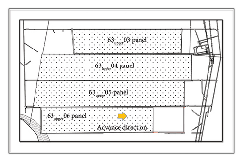
Among the four panels in the No. 6 mining area of the Dongtan coal mine, the 63upper03 panel experienced 727 mine earthquakes, with the largest event having an energy of 2.42 × 10⁶ J. The 63upper04 panel experienced 2187 mine earthquakes, with the largest event having an energy of 8.82 × 10⁶ J. The 63upper05 panel experienced 7857 mine earthquakes, with the largest event having an energy of 1.45 × 10⁷ J. As of November 2023, the 63upper06 panel has recorded 54 mine earthquakes with energy greater than 1 × 10⁵ J (strong mine earthquakes) and 715 events with energy greater than 1 × 10⁴ J. Compared to the other three panels in the No. 6 mining area, the 63upper06 panel has significantly higher numbers of both total mine earthquakes and strong mine earthquakes. The frequent occurrence of high-energy mine earthquakes in the 63upper06 panel poses a serious threat to the safety of underground miners and affects the production efficiency and economic benefits of mining operations.
3. Informer Time Series Forecasting Principles
Deep learning is a new research direction in the field of artificial intelligence, and it has been widely used in many fields such as computer vision, natural speech processing, and text recognition. The main feature of deep learning models is that they can extract feature information from data. By summarizing the changing characteristics of the training data, the model can create a more general pattern of change in the data and perform prediction tasks in various situations. What kind of tasks the deep learning model can perform depends entirely on the type of training data. The quality and quantity of data play a key role in deep learning.
The Informer is a supervised model based on multihead probabilistic attention mechanism, which consists of two parts: encoder and decoder, where the encoder is used to obtain long-term dependence on the robustness of the original input sequences, the decoder can realize the final time series prediction task, and the overall architecture is shown in Figure 2.
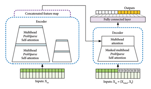
In addition, considering the importance of temporal information to the problem of time series forecasting, such as working days, holidays, different times of the day, etc., can have an impact on human activities. The Informer encodes (temporally embeds) information, such as month, year, moments, etc., of the sequence data, and the input of this global temporal information helps to improve the model’s ability to capture long-term dependencies. Eventually, the location and time embedding information is added to the transformed dimensionality of the impact factor data together into the model.
Both the encoder and decoder of the model receive data inputs, but the specifics differ. The input to the encoder is one long sequence from historical data (e.g., the first 24 h), while the input to the decoder consists of a combination of a short sequence (e.g., the first 12 h) and a zero-value equal to the predicted step size, where a value of 0 in the decoder input is used as a placeholder for the predicted value.
In the process of coal mining, mine earthquakes with varying energy sizes are monitored several times a day. So, in this study, the maximum mine earthquakes occurring every day since the mining of the 63upper06 panel are regarded as a time series with a fixed time interval of 1 day, and the maximum energy mine earthquakes are predicted every day by this deep learning model.
4. Data Preprocessing and Model Hyperparameters
First, FFT bandpass filtering was performed on all mine earthquake data to remove noise interference. All data containing mine earthquake signals were then extracted and organized into a specialized mine earthquake signal database. The date, time of occurrence, and sensor ID for each mine earthquake event were added to the database. The mine earthquake data were truncated to include 1000 data points before and after each mine earthquake signal. As shown in Table 1, a total of 2088 sets of clear mine earthquake data suitable for experimentation were obtained through this data organization. The clear signal database facilitates the author’s research on first-arrival time extraction; for comparative analysis, it is only necessary to extract data with the same ID from the database for each of the two methods being compared.
| Time of occurrence of the mine earthquake | Sensor ID | Mine earthquake data | |||||||
|---|---|---|---|---|---|---|---|---|---|
| 0 | 1 | 2 | 3 | 4 | 5 | 6 | … | ||
| 2019-12-31 07.39.09 | 17 | −0.0132 | −0.00859 | −0.00317 | 0.002493 | 0.007856 | 0.012416 | 0.015778 | … |
| 2019-12-31 07.54.43 | 15 | 0.023938 | 0.023888 | 0.019469 | 0.011569 | 0.001669 | −0.00842 | −0.01685 | … |
| 2020-01-01 01.18.57 | 12 | 0.001475 | 0.001574 | 0.001433 | 0.001069 | 0.000522 | −0.00014 | −0.00081 | … |
| 2020-01-01 01.18.57 | 15 | −0.00613 | −0.00865 | −0.01101 | −0.01288 | −0.01394 | −0.01393 | −0.01267 | … |
| … | … | … | … | … | … | … | … | … | … |
| 2021-02-06 05.29.24 | 15 | −0.00691 | −0.00767 | −0.00783 | −0.00726 | −0.00596 | −0.00395 | −0.00137 | … |
| 2021-02-06 07.54.40 | 12 | 0.023432 | 0.007296 | −0.00972 | −0.02556 | −0.03822 | −0.04591 | −0.04737 | … |
| 2021-02-06 07.54.40 | 15 | −0.00049 | 0.000594 | 0.001678 | 0.002701 | 0.003603 | 0.004326 | 0.004814 | … |
| 2021-02-06 10.38.42 | 6 | −0.00038 | −0.00925 | −0.01603 | −0.01961 | −0.01954 | −0.01604 | −0.00991 | … |
| … | … | … | … | … | … | … | … | … | … |
The sliding window energy ratio (RWR) method and the Akaike Information Criterion (AIC) method are both commonly used techniques for extracting the arrival time of microseismic signals. In order to ensure that the different first-arrival time extraction algorithms are highly comparable, the two methods are compared and analyzed as follows:
- 1.
First, the RWR method was used to extract the P-wave first-arrival times for the aforementioned 24 sets of data. The window size was set to 2, and the mutation threshold was set to 1.01. The calculation results are shown in Table 2.
-
Based on Table 2, the following results can be obtained:
- ①
For the P-wave first-arrival time extraction, the maximum absolute value of the time difference is 0.066 s, the minimum time difference is 0.002 s, the average time difference is 0.017 s, and the standard deviation of the time difference is 0.034 s.
- ②
The maximum computation runtime is 2.031095 s, the minimum computation runtime is 2.001985 s, the average computation time is 2.015589667 s, and the standard deviation of computation runtime is 0.007666772 s.
- ③
Among the 24 first-arrival time extraction results, there are 15 instances where the initial arrival times extracted using the RWR method occurred after the manually picked times.
- ④
There were no cases where the P-wave first-arrival time extraction failed.
- ①
- 2.
The AIC method was used to extract the P-wave first-arrival times from the same 24 sets of data. The calculation results are shown in Table 3.
-
Based on Table 3, the following conclusions can be drawn:
- ①
For the P-wave first-arrival time extraction, the maximum absolute value of the time difference is 0.074 s, the minimum time difference is 0.000 s, the average time difference is 0.024 s, and the standard deviation of the time difference is 0.053 s.
- ②
The maximum computation runtime is 2.171708 s, the minimum computation runtime is 2.031637 s, the average computation time is 2.1267845 s, and the standard deviation of the computation runtime is 0.0322254965 s.
- ③
Among the 24 first-arrival time extraction results, 21 instances extracted using the RWR method occurred before the manually picked times.
- ④
There were no cases where the P-wave first-arrival time extraction failed.
- ①
- 3.
A comparison of computational accuracy, computational speed, and computational stability between the two different methods is provided in Table 4.
-
The calculation results of the two methods have been compared and analyzed, and the following conclusions can be obtained:
- ①
The average time difference and the standard deviation of the time difference in first-arrival time extraction using the RWR method are both lower than those of the AIC method. This indicates that the RWR method has higher calculation accuracy compared to the AIC method.
- ②
The average computation time and the standard deviation of computation time for first-arrival time extraction using the RWR method are significantly lower than those of the AIC method. This suggests that the RWR method is faster in computation speed compared to the AIC method.
- ③
Based on the standard deviations of the time difference in first-arrival time extraction and the computation time, it can be concluded that the RWR method is more stable than the AIC method.
- ①
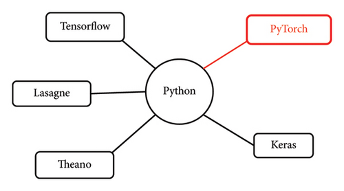
The task of deep learning using Python requires the help of extension libraries in it, and the most important deep learning libraries are Tensorflow, Lasagen, Theano, Keras, and PyTorch, as shown in Figure 3. The core idea of PyTorch is to represent nodes and edges on a computational graph through a data structure called a Tensor, and to construct computational graphs by combining these nodes and edges to achieve automatic derivation and back propagation. This section first describes the computational environment for this deep learning task, as shown in Table 5.
| Data ID | Manual picking time (s) | RWR calculated time (s) | Time difference (s) | Computation time (s) |
|---|---|---|---|---|
| 10 | 0.676 | 0.734 | −0.058 | 2.002757 |
| 42 | 0.598 | 0.584 | 0.014 | 2.004547 |
| 107 | 0.996 | 0.938 | 0.058 | 2.012014 |
| 120 | 0.424 | 0.464 | −0.040 | 2.012047 |
| 200 | 0.736 | 0.760 | −0.024 | 2.015192 |
| 322 | 1.006 | 1.004 | 0.002 | 2.016209 |
| 375 | 1.044 | 1.084 | −0.040 | 2.015121 |
| 436 | 0.246 | 0.274 | −0.028 | 2.015406 |
| 544 | 0.950 | 0.944 | 0.006 | 2.031095 |
| 563 | 1.020 | 1.018 | 0.002 | 2.001985 |
| 605 | 1.018 | 1.032 | −0.014 | 2.031075 |
| 657 | 1.036 | 1.046 | −0.010 | 2.015471 |
| 738 | 1.002 | 1.042 | −0.040 | 2.015444 |
| 876 | 1.008 | 1.074 | −0.066 | 2.007344 |
| 978 | 1.058 | 1.126 | −0.068 | 2.031022 |
| 1052 | 0.304 | 0.302 | 0.002 | 2.015154 |
| 1132 | 0.962 | 0.986 | −0.024 | 2.015466 |
| 1226 | 1.018 | 0.988 | 0.030 | 2.015449 |
| 1429 | 0.940 | 0.946 | −0.006 | 2.013462 |
| 1532 | 1.034 | 1.144 | −0.11 | 2.015478 |
| 1609 | 0.180 | 0.168 | 0.012 | 2.026605 |
| 1736 | 0.648 | 0.654 | −0.006 | 2.015211 |
| 1828 | 0.972 | 0.962 | 0.010 | 2.015474 |
| 1920 | 0.512 | 0.532 | −0.020 | 2.015124 |
| Data ID | Manual picking time (s) | RWR calculated time (s) | Time difference (s) | Computation time (s) |
|---|---|---|---|---|
| 10 | 0.676 | 0.654 | 0.022 | 2.140122 |
| 42 | 0.598 | 0.580 | 0.018 | 2.108993 |
| 107 | 0.996 | 0.958 | 0.038 | 2.124799 |
| 120 | 0.424 | 0.402 | 0.022 | 2.077910 |
| 200 | 0.736 | 0.722 | 0.014 | 2.124797 |
| 322 | 1.006 | 0.982 | 0.024 | 2.151223 |
| 375 | 1.044 | 1.036 | 0.008 | 2.131903 |
| 436 | 0.246 | 0.240 | 0.006 | 2.103341 |
| 544 | 0.950 | 0.940 | 0.010 | 2.134246 |
| 563 | 1.020 | 0.878 | 0.142 | 2.156044 |
| 605 | 1.018 | 1.002 | 0.016 | 2.156021 |
| 657 | 1.036 | 1.020 | 0.016 | 2.140683 |
| 738 | 1.002 | 1.004 | −0.002 | 2.155740 |
| 876 | 1.008 | 1.010 | −0.002 | 2.156058 |
| 978 | 1.058 | 1.056 | 0.002 | 2.171708 |
| 1052 | 0.304 | 0.302 | 0.002 | 2.061628 |
| 1132 | 0.962 | 0.962 | 0.000 | 2.140413 |
| 1226 | 1.018 | 0.944 | 0.074 | 2.138577 |
| 1429 | 0.940 | 0.928 | 0.012 | 2.138335 |
| 1532 | 1.034 | 1.142 | −0.108 | 2.155881 |
| 1611 | 0.180 | 0.166 | 0.014 | 2.031637 |
| 1736 | 0.648 | 0.458 | 0.190 | 2.109097 |
| 1828 | 0.972 | 0.962 | 0.010 | 2.124513 |
| 1920 | 0.512 | 0.464 | 0.048 | 2.109159 |
| Method | Average time difference in first-arrival time extraction (s) | Standard deviation of time difference in first-arrival time extraction (s) | Average computation time for first-arrival time extraction (s) | Standard deviation of computation time for first-arrival time extraction | Existence of zero time difference cases | Presence of failed first-arrival time extraction cases |
|---|---|---|---|---|---|---|
| RWR | 0.017 | 0.034 | 2.01558 | 0.00766 | Null | Null |
| AIC | 0.024 | 0.053 | 2.12678 | 0.03222 | One instance | Null |
| Configuration item | Versions |
|---|---|
| Programming language | Python 3.8 |
| Deep learning framework | PyTorch 1.8 |
| Computer system | Windows10 (64 bit operating system) |
| RAM | 16 GB |
| CPU | Intel (R) Core (TM) i9-13900 HX |
| GPU | NVIDIA GeForce RTX 4050Laptop GPU |
Mine earthquakes have the basic characteristics of high frequency and low energy. Since the number of microseismic events is not the same every day, and the time difference between the occurrence of two or two mine earthquakes is not the same, this makes the task of time series prediction more difficult. Pre-processing of the ore-seismic data is required. The data processing for this prediction task is carried out in the following ways.
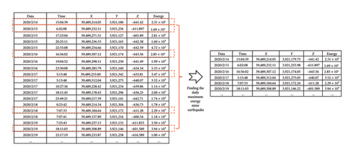
The collected data from February 14, 2020, to October 4, 2023, contained a total of 12,237 mine earthquakes, from which the maximum energy mine earthquake per day, denoted as Emax, is extracted. The time-series dataset with an interval of 1 day is approximated from the time of mining to the present day, and the mechanism of data processing and the form of the processed data are shown in Figure 4. Among them, training set: 80% of the data, covering the earliest period to facilitate model learning of historical patterns. Validation set: 10% of the data, used during training to tune hyperparameters (e.g., sequence length, learning rate) and prevent overfitting. Test set: 10% of the most recent data, reserved for final performance evaluation to ensure unbiased metrics. This split aligns with common practices in time-series research, where chronological ordering is preserved to mimic real-world prediction scenarios (i.e., predicting future events based on past data).
The Informer time series prediction can be multivariate predicting multivariate, multivariate predicting univariate, and univariate predicting univariate. When making predictions with multivariate data, the methodology is classified as supervised learning. In contrast, predicting with univariate data falls under unsupervised learning. This paper employs a univariate predictive model for the purpose of prediction. After many attempts, the remaining hyperparameters are chosen to be suitable for the prediction of each type of mine earthquakes’ data, as shown in Table 6.
| Parameter name | Parameter selection | Parameter function |
|---|---|---|
| --seq_len | 256/128/64 | Input sequence length |
| --label_len | 128/64/32 | A priori knowledge length |
| --label_len | 64/32/16 | Predicted sequence length |
| --enc_in | 3 | Feature parameter |
| --dec_in | 3 | Characterization parameter |
| --c_out | 3 | Decoder feature parameters |
| --e_layers | 3 | Encoder parameters |
| --d_layers | 3 | Decoder parameters |
| --d_model | 516 | Hidden layer features |
| --d_ff | 2048 | Number of neurons in the fully connected layer |
| --n_heads | 8 | Multiple head mechanism |
| --factor | 8 | Sampling factor |
| --dropout | 0.05 | Neural network regularization operation |
| --learning_rate | 0.0001 | Learning rate |
| --train_epochs | 10 | Number of training rounds |
In order to ensure the reliability and accuracy of the proposed model, several metrics are used to comprehensively evaluate the used mine earthquakes’ dataset and the proposed model. These metrics include mean square error (MSE), mean absolute error (MAE), mean absolute percentage error (MAPE), and root mean square error (RMSE). The specific formulas and meanings of these indicators are detailed in Table 7. In the process of model evaluation, the closer the value of the indicator is to 0, the better the performance of the tested model. Where n represents the number of rock burst characterization data, and y and ŷ denote the ith data of measurement and prediction of rock burst characterization in the experiment, respectively.
| Assessment indicators | Calculation formula | Physical meaning |
|---|---|---|
| MSE | Mean square error ratio of predicted values | |
| MAE | Mean absolute error ratio of forecasted values | |
| MAPE | Mean absolute percentage error ratio of forecasts | |
| RMSE | Root-mean-square error ratio of forecasts |
5. Informer Time-Series Prediction of Mine Earthquakes
5.1. Daily Maximum Energy Mine Earthquake Prediction System
The time series prediction of the largest daily energy mine earthquake will be univariate prediction from the horizontal coordinate, vertical coordinate, seismic source depth, and seismic source energy of the largest daily mine earthquake, which will be combined to form a complete prediction system, as shown in Figure 5.
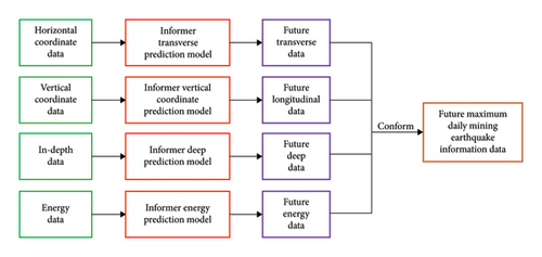
The four models depicted in Figure 5 predict the horizontal, vertical, depth, and energy of a mine earthquake from top to bottom. The four models have the same data input format and similar internal models, but their predictions are independent and not linked to each other. The models are trained separately based on the different dimensions of the predicted data given, and they divided their work so that each model would only predict one dimension of information in the location of the source of the mine earthquake. This information is finally integrated to obtain the complete source location information of the mine earthquake for a certain period of time in the future. The advantage of such a process is that it can improve the accuracy of the prediction of the source location of the mine earthquake. If a single model is designed to directly predict all the information about the source location of a mine earthquake, it will lead to an uncontrollable error in the model prediction. However, if multiple models collaborate with each other and perform their own duties, a single model only needs to focus on the information of the dimension it is responsible for, and only pay attention to the change rule of data in one dimension, so as to achieve the purpose of improving the accuracy. For example, the model responsible for predicting the energy of the mine earthquake only needs to focus on how the energy changes.
For the mine earthquake, there is a certain correlation between the occurrence of an adjacent mine earthquake, and this imperceptible correlation can be mined through the deep learning method, so that the maximum energy of the mine earthquake occurring in the 63upper06 panel from the mining of 1435 days to the present day is predicted. The training set, validation set, and test set each account for 0.8, 0.1, and 0.1, respectively, where the training set is used for the training of the model, the validation set is used for the model itself to test itself in each round of training and adjust the parameters, and the test set is used to test the prediction effect at the end of 10 rounds of training.
5.2. Daily Maximum Energy Mine Earthquakes’ Source Information Prediction
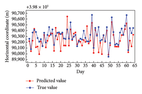
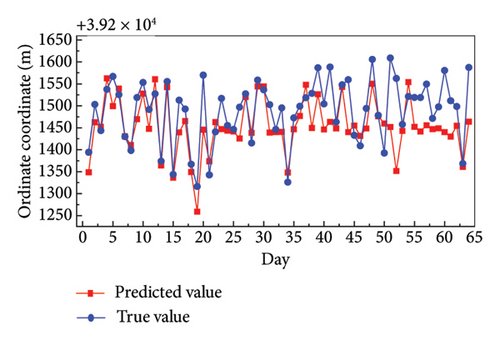
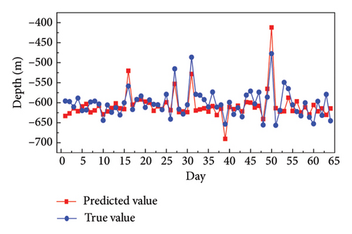
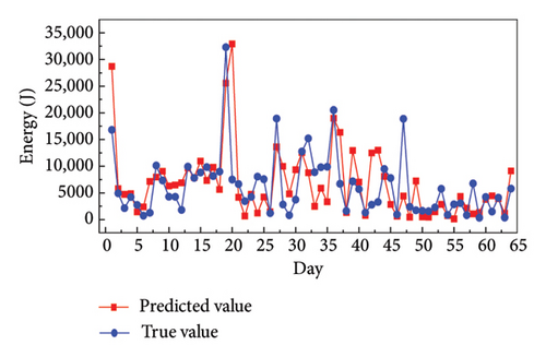
The predicted effects of the 64-day daily maximum energy mine earthquakes are shown in Figure 6, and the predicted effects are evaluated in Table 8.
| Mine earthquakes’ source information | MSE | RMSE | MAPE | MAE |
|---|---|---|---|---|
| Horizontal coordinates | 16,300.83 | 127.67 | 0.001 | 95.97 |
| Vertical coordinates | 3961.11 | 62.94 | 0.031 | 46.63 |
| Depth | 666.30 | 25.81 | 0.036 | 21.06 |
| Energy | 30,501,244.88 | 5522.79 | 0.97 | 3666.76 |
From Figure 6, it can be seen that the Informer model has the best fit for the prediction of depth and the worst fit for the prediction of energy. From Table 8, the evaluation indexes of the Informer model show that the MAE of the model is the lowest in the prediction of depth, the MAPE of the model is the lowest in the prediction of horizontal coordinates, and the MAPE of the Informer model for the prediction of seismic source coordinates is within 5%, which is within the acceptable range of error. Combining the two methods of visual judgment and evaluation index judgment, the Informer model is more suitable for the prediction of epicenter location coordinates and less effective for the prediction of energy in the prediction of the maximum daily energy of mine earthquakes in the next 64 days.
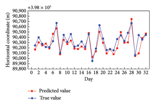
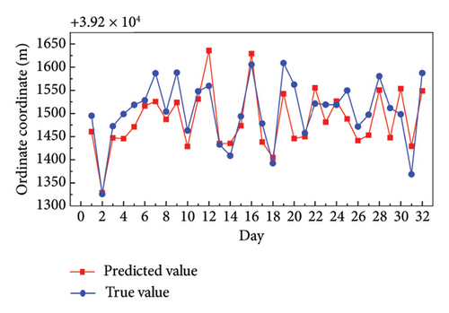
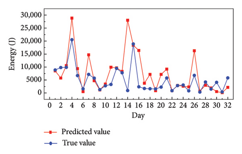
The predicted effects of the 32-day daily maximum energy mine earthquakes are shown in Figure 7, and the predicted effects are evaluated in Table 9.

| Mine earthquakes’ source information | MSE | RMSE | MAPE | MAE |
|---|---|---|---|---|
| Horizontal coordinates | 10,236.19 | 101.17 | 0.00085 | 77.41 |
| Vertical coordinates | 2074.67 | 45.54 | 0.025 | 38.23 |
| Depth | 575.86 | 23.40 | 0.030 | 18.76 |
| Energy | 41,194,349.98 | 6418.28 | 1.742 | 3536.31 |
From Figure 7, it can be seen that the Informer model has the best fit for the prediction of transverse coordinates and depth, and the worst fit for the prediction of energy. From Table 9, the evaluation indexes of the Informer model show that the MAE is the lowest in the depth prediction, the MAPE is the lowest in the transverse prediction, and the MAPE of the Informer model for the location of the seismic source is within 3%, which is within the acceptable range of error. Combining the two methods of visual judgment and evaluation index judgment, the Informer model is more suitable for the prediction of the coordinates of the epicenter location and less effective for the prediction of the energy in the prediction of the daily maximum energy mine earthquake in the next 32 days.
Compared to the results of the prediction of the daily maximum energy mine earthquake for the next 64 days using the Informer model, the MSE in the horizontal coordinate is reduced by 37.2%, RMSE is reduced by 20.8%, MAPE is reduced by 15.0%, and MAE is reduced by 19.3%; the MSE in the vertical coordinate is reduced by 47.6%, RMSE is reduced by 27.6%, MAPE is reduced by 19.4%, and MAE is reduced by 18%; MSE in depth is decreased by 13.6%, RMSE is decreased by 9.3%, MAPE is decreased by 16.7%, and MAE is decreased by 11.4%. It can be seen that the prediction effects of the coordinates of the seismic source location have all been improved to some extent. However, the prediction of the energy of the mine earthquake is significantly worse, and in terms of the prediction of the source location coordinates, the prediction of 32 days is significantly better than the prediction of 64 days.
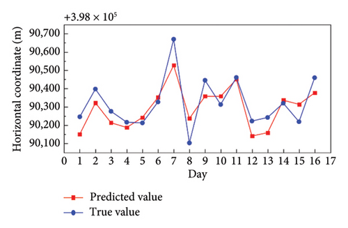
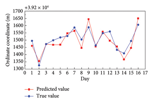
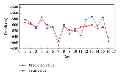
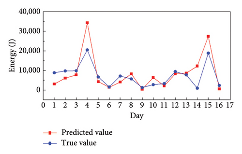
The predicted effects of the 16-day daily maximum energy mine earthquakes are shown in Figure 8, and the predicted effects are evaluated in Table 10.
| Mine earthquakes’ source information | MSE | RMSE | MAPE | MAE |
|---|---|---|---|---|
| Horizontal coordinates | 50,264.16 | 224.19 | 0.002 | 183.50 |
| Vertical coordinates | 7131.47 | 84.44 | 0.045 | 69.50 |
| Depth | 682.36 | 26.12 | 0.034 | 21.31 |
| Energy | 144,766,158.12 | 12,031.88 | 1.92 | 10,416.90 |
From Figure 8, it can be seen that the Informer model works best for the prediction of trends in vertical coordinates and depth, and worst for depth change trends. From Table 10, the evaluation indexes of the Informer model show that the MAE of the Informer model is the lowest in the prediction of depth, the MAPE is the lowest in the prediction of horizontal coordinate, and the MAPE of the Informer model for the location of the seismic source, which is the average absolute percentage error, is within 5%, which is within the acceptable range of error. Combining the two methods of visual judgment and evaluation index judgment, the Informer model is more suitable for the prediction of the coordinates of the epicenter location and less effective for the prediction of the energy in the prediction of the maximum daily energy of mine earthquakes in the next 16 days.
Three comparison tests are carried out above, and the task of deep learning prediction is performed on the data from the 63upper06 panel, respectively, to predict the daily maximum energy mine earthquake for the next 64 days, the daily maximum energy mine earthquake for the next 32 days, and the daily maximum energy mine earthquake for the next 16 days. The following conclusions can be obtained: the Informer time series prediction model predicts the source location coordinates of the possible future daily maximum energy mine earthquakes from the historical daily maximum energy mine earthquakes’ data. The Informer time series prediction model has the best prediction effect on the daily maximum energy mining quake for the next 32 days in the prediction task, in which the best prediction effect is for the horizontal coordinate, and the MAPE value of 0.00085 is the lowest among the three experiments.
6. Discussion
From the previous analysis, it can be seen that, for the prediction of dynamic disasters, scholars at home and abroad have done a lot of research in the field of coal bump and sudden water surge prediction, but the research on the prediction of mine earthquake has just started, and there is no conclusive conclusion as to what method can be used for mine earthquake prediction. Meanwhile, with the gradual rise of artificial intelligence big data, various algorithms such as machine learning and deep learning have been applied to the field of mine earthquake prediction. In this context, this paper takes the 63upper06 panel in the No. 6 mining areas of the Dongtan coal mine as the engineering background, and considers the maximum mine earthquake occurring every day since the mining of the 63upper06 panel as a time series, with a fixed time interval of 1 day, and predicts the maximum energy mine earthquake every day through the Informer deep learning model. The analysis shows that the results of the Informer model for the 63upper06 panel in the Dongtan coal mine are better. However, because of the different geological conditions and stress environments of each mine, the Informer modeling results of the 63upper06 panel cannot be applied to other coal mines, and the Informer modeling results of the 63upper06 panel cannot be completely copied, but the Informer modeling results of the 63upper06 panel can provide a reference for the blasting program of other coal mines. The Informer model mine earthquake prediction scheme of the 63upper06 panel can provide reference for other coal mines. In addition, the research on the application of deep learning in mine earthquake in this paper is limited to only one method. There are still a large number of AI methods waiting to be studied, and the AI big data methods rely on a large amount of data, while the data and methods used in this mine earthquake are limited. For this reason, in the next research, we will strengthen this aspect of the research.
In summary, with the rise of artificial intelligence algorithms, machine learning as well as deep learning algorithms are widely used in various industries because of their fast classification ability. In this study, based on the mine earthquake data from the No. 6 mining areas of the Dongtan coal mine, machine learning methods were used to construct a scientific prediction model, analyze the historical mine earthquake data, and carry out a mine earthquake prediction study. At the same time, this study aims to improve the accuracy of mine earthquake early warning and provide a certain theoretical basis for the safety management of mine production, so as to promote the safe production and sustainable development of the mining industry.
7. Conclusions
- 1.
The Informer time-series prediction model predicts the source location coordinates of the potential future daily maximum-energy mine earthquakes from the historical daily maximum-energy mine earthquakes’ data.
- 2.
The Informer time series prediction model performs better in the task of mine earthquake prediction, and the prediction of the location of the source of the mine earthquake is better than the prediction of the size of the energy of the mine earthquake.
- 3.
The Informer time series prediction model predicts the maximum daily energy of the mine earthquake in the next 32 days with the best results, and the medium-long sequence of 32 days has the best results compared with the short sequence of 16 days and the long sequence of 64 days.
Conflicts of Interest
The authors declare no conflicts of interest.
Funding
This work was supported by the Taishan Industrial Experts Program (No. tscx202408130) and Shandong Energy Group (No. SNKJ2022A01-R26).
Open Research
Data Availability Statement
The data used to support the findings of this study are available from the corresponding author upon reasonable request.


