Application of Intelligent Low-Cost Accelerometers for Bridge Monitoring With a Deep Learning Approach
Abstract
Despite the crucial role of structural health monitoring (SHM) in ensuring the integrity and safety of essential infrastructure, its adoption is often limited by the high costs of traditional sensors. This study introduces an innovative approach for creating intelligent, high-performing low-cost accelerometers using a deep learning framework rooted in long short–term memory (LSTM) neural networks. Initially, commercial sensors are temporarily installed alongside low-cost accelerometers on a bridge to facilitate the training process. Once the training is complete, the commercial sensors are removed, leaving the calibrated low-cost accelerometers permanently in place to perform continuous SHM tasks. In a case study, a bridge was equipped with an array of six low-cost and six commercial sensors. The efficacy of this innovative approach is corroborated through a comparative analysis of mode shapes and eigenfrequencies derived from both the low-cost and commercial sensors, as well as intelligent low-cost accelerometers.
1. Introduction
The onset of the fourth industrial revolution, Industry 4.0 [1], signifies a transformative period for structural and construction engineering. This era, marked by the digital revolution, introduces Construction 4.0, a concept that embodies the integration of emerging trends and technologies [2]. These innovations promise to redefine the lifecycle management of built environment assets from design and construction to maintenance [3]. Central to this transformation are artificial intelligence (AI) tools [4], which span machine learning, optimization algorithms, computer vision, and deep learning. Such tools are revolutionizing decision-making processes, presenting sophisticated solutions to the sector’s complex challenges [5].
In recent years, there has been a growing interest in the use of AI in all engineering domains and it has fueled many visions and hopes [6]. The incorporation of AI in civil engineering [7] has seen a significant impact, a testament to its potential in enhancing various aspects of the field [8]. This includes the comprehensive application of AI for nondestructive testing, sensor data analysis, finite element simulations, and structural inspections [9]. AI’s capability to address problems beyond the reach of traditional computational methods signifies a paradigm shift, offering a multifaceted approach to engineering challenges [10]. The increasing adoption and application of AI tools in this sector are well-supported by literature [11], with numerous studies and reviews highlighting their impact. For instance, the research conducted by Huang et al. [12] shows the increasing use of big data and deep learning technologies in various fields of civil engineering. Wang et al. [13] developed a machine learning–based anomaly detection method for online bridge monitoring, which identifies both interperiod and intraperiod correlations in sensor data to enhance the accuracy of anomaly detection. Several -scholars have explored the use of AI in civil engineering [14, 15].
Structural health monitoring (SHM) [16] emerges as a prime area benefitting from AI’s prowess [17]. Traditionally reliant on manual inspections and conventional sensors [18], SHM’s evolution toward AI–enhanced methodologies marks a shift toward more efficient, proactive monitoring strategies [19]. This advancement allows for the real-time processing of vast sensor datasets [20], enabling prompt identification of structural anomalies [21]. The contributions and future directions of AI in SHM have been reviewed and discussed in the works by Sun et al. [17] and Salehi and Burgueño [22], highlighting the evolving challenges and trends in utilizing AI tools for these purposes [23].
In the realm of SHM [24], accelerometers play a crucial role, offering insights into the dynamic behavior and stability of structures [25]. Despite the high cost associated with advanced sensor technology limiting their widespread application [26], the last decade has witnessed a growing interest in exploring affordable sensor technologies [27]. Low-cost accelerometers [28], for instance, provide a viable alternative for extensive SHM applications [29], given their affordability and adaptability for large-scale deployments and integration into the existing monitoring frameworks [30].
Rocha Ribeiro et al. [31] developed a low-cost wireless multinode vibration monitoring system for SHM using Arduino-based technology, designed to be technically accessible and scalable. Talebi-Kalaleh et al. [32] introduced an innovative damage detection framework for bridge structures that leverages compressed sensing (CS) of crowdsourced acceleration data collected from smartphones in vehicles. This framework effectively addresses challenges in traditional SHM methods, such as high costs and complex sensor installations, by integrating CS to reduce data collection requirements while preserving critical damage-sensitive information. These works demonstrate the feasibility of deploying low-cost SHM systems for practical applications, providing an open-source framework to facilitate adoption even by nonspecialists. Sakr et al. developed an innovative framework integrating Arduino-based Internet-of-Things (IoT) sensors and building information modeling (BIM) for SHM. The study utilized Arduino microcontrollers to address real-time visualization challenges in SHM by creating an IoT sensor system that autonomously collects, processes, and visualizes data within a BIM environment [33]. Goyal and Pabla designed an Arduino-based noncontact SHM system for machine tools, leveraging a microcontroller platform and light-dependent resistors (LDRs). The system measures vibrations without requiring direct contact, enabling cost-effective and real-time condition monitoring [34].
However, the adoption of low-cost microelectromechanical system (MEMS) [31] accelerometers is not without challenges [35], primarily concerning their accuracy and resolution compared to commercial alternatives. Consequently, a prominent research gap exists around methods to calibrate and refine the accuracy of data acquisition from these economical devices. This issue is paralleled by the demand for sophisticated data postprocessing tools aimed at enhancing signal quality [36].
- •
Low-pass filters, which selectively permit frequencies below a predefined threshold while attenuating higher frequencies, thereby minimizing high-frequency noise interference in sensor data [38].
- •
High-pass filters, which are designed to eliminate low-frequency noise and drift by permitting only frequencies above a specific threshold [39].
- •
Band-pass filters, which merge low-pass and high-pass filter principles to isolate signals within a particular frequency range [40].
- •
Band-stop filters, which target the removal of frequencies within a defined range while allowing all others [41].
- •
Butterworth filters, which are valued for their smooth, ripple-free signal in the passband [42].
- •
Wavelet denoising [43], which employs wavelet transforms for selective noise reduction, maintaining essential signal details.
- •
Kalman Filters [44], which is a sophisticated approach that estimates variables from noisy measurements over time.
Delving into these filtering techniques is vital as the domain of SHM becomes more congested, emphasizing the continued effort to efficiently utilize low-cost sensors [45] in SHM without degrading data quality. It is noteworthy that these techniques are applicable to both economical and high-end commercial sensors [36]. A significant gap remains for a system or application expressly tailored for low-cost sensors to improve, calibrate, or enhance them, as utilizing the mentioned filters can also benefit commercial sensors, potentially exacerbating the resolution and accuracy disparities between low-cost and high-end sensors. This highlights the need for specialized solutions that cater to the unique challenges of low-cost sensors, aiming to narrow the performance gap and make SHM more accessible and cost-effective.
Furthermore, there are additional gaps in the literature, including the underutilization of low-cost systems for operational modal analysis (OMA) [46] of complete bridge structures [47]. Recent advancements in integrating machine learning techniques with OMA have shown significant potential for improving SHM systems. Civera et al. [48] proposed a machine learning–based automatic OMA framework combining stochastic subspace identification (SSI) with clustering methods to address spurious mode identification, demonstrating its applicability to masonry arch bridges under progressive damage scenarios. Similarly, Mugnaini et al. [49] introduced a machine learning approach for automating OMA by integrating SSI with clustering algorithms such as k-means and hierarchical clustering, enabling efficient modal parameter identification in noisy conditions. These studies underscore the growing role of machine learning in enhancing the scalability and automation of SHM processes, serving as a foundation for further advancements in this domain.
In addition, there is a lack of exploration into the novel application of deep learning algorithms for enhancing vibration acquisition. Another critical gap involves the calibration of low-cost accelerometers using commercial sensors, aiming to improve the time-domain acquired data of low-cost sensors through deep learning algorithms. It is essential to evaluate the modal values of the structure in the frequency domain to ensure that overfitting does not occur. Overfitting is a common issue in machine learning where a model learns the training data too well, including the noise or irrelevant details, and fails to generalize to new, unseen data. This approach enables the calibration of sensors, rather than merely enhancing their data through postprocessing methods.
To address these limitations, this paper introduces a novel approach involving the use of an AI–driven tool, specifically a long short–term memory (LSTM) model [50]. LSTM networks are a type of recurrent neural network (RNN) designed to capture long-term dependencies in sequential data, making them particularly effective for sequential data and ideal for time-series analysis of sensor measurements. In contrast, other AI algorithms such as convolutional neural networks (CNNs) require padding or truncation when working with variable-length sequences, potentially losing information or introducing artifacts, as CNNs are primarily used for spatial data processing, excelling in tasks such as image and video recognition by detecting local patterns through convolutional layers [51]. Compared to traditional RNN, LSTM mitigates the vanishing gradient problem by introducing gating mechanisms (input, forget, and output gates). This allows them to maintain gradients over long sequences, and unlike standard RNNs, the gating mechanism in LSTMs allows selective forgetting of irrelevant or noisy information, making them more robust in real-world scenarios where there are inherent noise in recorded data [52]. These distinctions highlight LSTM’s unique capability to model temporal dynamics, setting it apart from algorithms such as CNNs and SVMs, which are not inherently designed to handle sequential dependencies [53].
This model is specifically designed to enhance and calibrate low-cost MEMS accelerometers on a bridge by provisionally installing commercial sensors during the training phase. The ultimate goal is to achieve intelligent sensing, demonstrating that low-cost sensors, when augmented with AI, can provide a viable alternative to more expensive commercial sensor systems without compromising data quality and accuracy. In addition, once the training phase is completed, the enhanced data acquisition from the low-cost accelerometers can be managed through cloud computing on an IoT platform, or directly on a Raspberry Pi serving as the data acquisition system.
The structure of this paper is outlined as follows. Section 2 elaborates on the LSTM algorithm for sensor data enhancement, including the development process of the intelligent LARA (ILARA). Section 3 presents a case study that utilizes both LARA and commercial sensors for the instrumentation of a bridge, showcasing the practical application of these technologies. In Section 4, a comparative analysis of modal estimations derived from LARA, ILARA, and commercial sensorsis presented together with a detailed discussion of the findings. Finally, Section 5 concludes the paper by summarizing the key outcomes and proposing directions for future research.
2. The Development and Application of the ILARA Using LSTM
The proposed AI tool is based on an LSTM model, which offers a powerful solution for addressing challenges and enhancing the accuracy of models trained on data with time-series dependencies such as inclinometers and accelerometers [54, 55]. LSTM networks are distinguished from other types of RNNs by an architecture specifically designed to address the vanishing gradient problem, which often hinders the training of traditional RNNs on long sequences of data. Unlike traditional machine learning algorithms that struggle to capture temporal dependencies in sequential data, LSTM networks excel at modeling complex temporal dynamics by maintaining long-term dependencies and mitigating the effects of noise and irregularities. It should be noted that a key feature of LSTM that makes it suitable for this study is its ability to effectively handle time-series data with irregular sampling rates. Low-cost sensors often produce data streams characterized by nonuniform time intervals between consecutive measurements [56]. LSTM networks are inherently capable of learning from such irregularly sampled data, as they can adaptively adjust their internal state based on the timing and sequence of observations. This adaptability allows LSTM networks to effectively capture the temporal patterns inherent in sensor data, thereby improving the prediction accuracy compared to traditional methods. Furthermore, LSTM networks are well-suited for handling noisy sensor data and mitigating the impact of sensor drift [57]. LSTM networks can filter out noise and extract meaningful signal features from noisy sensor measurements by learning to retain relevant information over extended time intervals while selectively discarding irrelevant information. This noise-filtering capability enhances the robustness of predictive models trained on data from low-cost sensors, leading to more accurate and reliable predictions. Moreover, LSTM networks possess the ability to capture long-term dependencies in sequential data, which is particularly advantageous for applications where sensor measurements exhibit complex temporal dynamics. LSTMs are equipped with specialized memory cells and gating mechanisms that enable them to effectively capture and retain information over extended time intervals. By leveraging their memory cells to store and propagate information over extended time horizons, LSTM networks can capture subtle patterns and trends in sensor data that may span multiple time steps. This capability enables LSTM–based models to achieve superior accuracy in forecasting and anomaly detection tasks, even in the presence of challenging sensor characteristics. This AI tool has been extensively employed across a diverse range of applications, including prediction of material properties [58], comfort assessment [59], evaluation of structural performance [60], and energy consumption prediction in buildings [61]. Another advantage of using the LSTM model for this specific problem is its ability to handle time-series data, with processing feasibly conducted on a Raspberry Pi within the LARA system. Furthermore, the model can also be utilized for cloud computing on the IoT platform of ThingSpeak. It is important to note that more complex or ensemble models are not feasible due to the limited processing capabilities of the currently available Raspberry Pi 4.
2.1. LSTM Architecture
- •
TensorFlow, an open-source deep learning framework developed by Google Brain [62], is widely used due to its adaptability across multiple hardware platforms and its ability to support the development of complex neural network architectures.
- •
Keras is a high-level neural network application programming interface (API) that simplifies rapid prototyping and experimentation. By offering user-friendly building blocks, Keras enables researchers to concentrate on higher-level model design and data analysis rather than low-level implementation details.
The combined use of TensorFlow and Keras streamlined the construction of the LSTM network, leveraging their comprehensive features and optimizations. TensorFlow’s widespread adoption across different domains underscores its reliability and scalability in real-world applications [63].
The LSTM model aims to enhance the accuracy of a low-cost accelerometer system, known as LARA, by using data from commercial PCB sensors (considered a reference for higher precision). This refined model output is then used to determine the modal shapes of structures in a vibration analysis context. Specifically, data from six commercial sensors (PCB) and three LARA sensors were incorporated into this study. The placement and utilization of these sensors were customized for the data from this case study, with further details provided in subsequent sections.
- •
Input layer: This layer consists of six neurons corresponding to normalized sensor readings obtained from three LARA accelerometers and three PCB accelerometers. For signal enhancement and calibration, this structure enables the model to identify and learn correlations between the two sensor types.
- •
Data normalization: The StandardScaler method is employed to normalize data that includes outliers. This technique ensures that all features are scaled to have a mean of zero and a standard deviation of one, thereby standardizing the input data. Normalization helps mitigate the impact of varying scales among features, reduces sensitivity to extreme values (outliers), and accelerates the convergence of the model during training. By transforming the data into a consistent range, the LSTM model can better capture patterns and relationships, leading to improved accuracy and robustness in predictions.
- •
LSTM layers: The network’s core comprises one or more LSTM layers, each containing specialized units that can store information over time.
- 1.
Memory cell and gates: Each LSTM unit contains a memory cell and three types of gates (input, forget, and output). These gates work together to manage the flow of information at each time step, helping the model capture both short-term and long-term dependencies in sensor data.
- 2.
Vertical stacking: By stacking multiple LSTM layers, we allow deeper feature extraction. Each layer passes its hidden state to the next layer, progressively refining the learned representations.
- 1.
- •
Regularization: In this study, dropout layers were not used at the input or output. Dropout is often used to mitigate overfitting by randomly deactivating neurons during training. However, based on our preliminary experiments and dataset size, we opted to exclude it.
- •
Output layer: The final layer has three neurons, corresponding to the enhanced outputs for the three LARA accelerometers. These outputs aim to approximate the more accurate PCB measurements. By comparing the LARA outputs to the known PCB data during training, the LSTM learns how to correct or refine the LARA signals.
- •
Additional architectural details: It is noted that attention mechanisms, bidirectional LSTMs, gradient clipping, scheduled sampling, and ensemble methods are not incorporated in this study.
The architecture of the network is specifically customized based on the data from the case study, further details of which are provided in the following sections.
2.2. Advancements in Intelligent Low-Cost Sensor Monitoring System
In this section, the application of low-cost sensors in SHM and their significance in the industry are introduced. The review begins with a discussion on the state-of-the-art use of various low-cost sensors for SHM, specifically focusing on bridges. Subsequently, LARA, a standout low-cost accelerometer, is presented alongside its recent enhancements, with an in-depth look at its hardware and software components.
Commercial accelerometers are highly regarded in academic and industry circles for their widespread availability, dependability, and proven performance metrics [64]. One of their major benefits is the thorough calibration and validation processes they undergo. Manufacturers meticulously test and calibrate these devices to guarantee precise and consistent data, giving researchers a solid foundation for their monitoring projects and analysis [65]. The detailed specifications and performance indicators available for commercial accelerometers are the key factors in their broad acceptance within the scientific community.
Accelerometers hold a vital role in the SHM of bridges and buildings [66]. Essential characteristics of commercially available accelerometers, including name, acceleration range, frequency range, spectral noise density, price (VAT excluded), axis, and references, are summarized in Table 1. It is noteworthy that certain accelerometers, such as PCB TLD356A17 and PCB 356B18 shown in Table 1, require additional data acquisition equipment, which averages a cost of €700 per channel. The rest of the sensors introduced in this table generally do not need extra data acquisition equipment under the circumstances indicated on their datasheets.
| Model | Acceleration range (g) | Frequency range (Hz) | Spectral noise (μg/√Hz) | Price (€) | Axis | References |
|---|---|---|---|---|---|---|
| IOLITEi0-3x-ACC | ±8 | 0.0–1000.0 | 25 | 1820 | Triaxial | [67] |
| PCB TLD356A17 | ±10 | 0.5–3000.0 | 2.0 | 1750 | Triaxial | [68] |
| PCB 356B18 | ±5 | 0.5–3000.0 | 1.2 | 1460 | Triaxial | [36] |
| M604B31 | ±50 | 0.5–5000.0 | 5.0 | 700 | Triaxial | [69] |
| LARA | ±2 | 0.0–175.0 | 50.5 | 200 | Triaxial | [70] |
| MPU9250 | ±2 | 0.0–42.0 | 400.0 | 160 | Triaxial | [71] |
| ADXL335 | ±2 | 0.0–50.0 | 300.0 | No data | Triaxial | [72] |
| LEWIS2 | ±2 | 0.0–250 | 150.0 | No data | Triaxial | [73] |
| ADXL362 | ±2 | 0.0–50.0 | 400.0 | No data | Triaxial | [74] |
The analysis of the commercial solutions in Table 1 reveals a significant price variation, ranging from €700 to €1820. Accelerometers with higher prices (such as IOLITEi0-3x-ACC) usually provide a lower measurement range and higher resolution.
Civil engineering literature suggests that short-span bridges (with spans not exceeding 40 m [70]) primarily exhibit natural frequencies between 3.0 and 30.0 Hz [75]. Conversely, medium-to-long-span bridges display primary eigenfrequencies ranging from 0.1 to 8.0 Hz [76], underscoring the suitability of sensors with a more modest frequency range for SHM applications that demand lower acceleration ranges [77].
A prominent strategy in developing affordable accelerometers is leveraging MEMS sensors [78]. MEMS accelerometers present a cost-effective, low-power, and sensitive alternative with a sufficient sampling rate compared to their piezoelectric [79] counterparts [28]. Their ability to connect to economical microcontrollers, such as Arduino (known for its various communication ports, including the interintegrated circuit [I2C]) further underscores their utility [80].
The landscape of low-cost MEMS accelerometers is continually enriched by emerging prototypes. For instance, Pardeshi et al. [81] employed an ADXL335 accelerometer alongside an Arduino Mega2560 to assess vehicle tire pressure through wheel hub vibrations. Similarly, Patange et al. [81] devised a mechanism for identifying different failure modes in single-point cutting tools, utilizing machine learning and Arduino-based vibration detection equipment featuring an ADXL335 MEMS accelerometer.
Despite their versatility and benefits, MEMS accelerometers inherently exhibit higher noise density values compared to other accelerometer types [82]. Furthermore, unlike piezoelectric accelerometers that necessitate costly, precision external signal conditioning, MEMS accelerometers integrate this feature onboard, a factor that can introduce additional noise [70].
To mitigate the accuracy limitations typically associated with low-cost accelerometers, Komarizadehasl et al. [70] developed the LARA, distinguishing itself with the employment of five MPU9250 MEMS accelerometers to amplify performance. A comparative analysis in Table 1 highlights LARA’s significantly lower noise density (50.5 μg/√Hz) against alternatives such as the ADXL345 (300 μg/√Hz) [83], suggesting a notable advancement in reducing noise interference.
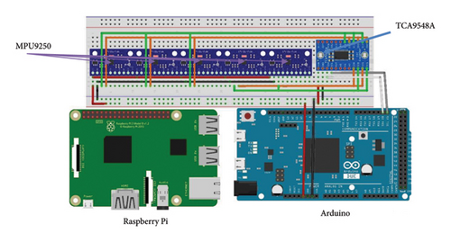
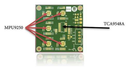
LARA signifies an innovative leap in cost-efficient sensor technology, incorporating open-source prototyping platforms, namely, Arduino and Raspberry Pi, alongside the economical MEMS accelerometer MPU9250. Though such accelerometers are rarely used in civil engineering due to precision concerns, LARA’s innovative approach (averaging readings from five accelerometers at a singular point through a multiplexer) marks a pioneering effort in literature to reduce overall noise density, balancing the signal-to-noise ratio [84] with the optimal number of accelerometers to maintain system sampling frequency.
Figure 1 details LARA’s sensor configurations, showcasing both the wiring setup with an Arduino Due microcontroller and its compact form. Through processing data from these devices, LARA corrects individual accelerometer discrepancies, achieving a precision akin to commercial-grade sensors. Its efficacy for dynamic monitoring of structures such as buildings and bridges has been affirmed.
To enhance usability, LARA’s framework has been reimagined to autonomously begin data collection upon power connection, ceasing after 2 min. Employing a Raspberry Pi, it establishes internet connectivity via Wi-Fi, LAN, or SIM card, accessing a Google Drive to download Python scripts for data acquisition. This setup ensures data management efficiency, with programmed tasks facilitating regular data transfer to Google Drive, thus preventing local storage overload. This innovative information flow, depicted in Figure 2(a), outlines LARA’s operation from initialization to data processing, showcasing its adaptability and precision-enhancement capabilities for SHM.

- a.
LARA initialization: Upon activation, LARA establishes an internet connection using Wi-Fi, LAN, or a SIM card, depending on the availability and compatibility of preconfigured network credentials.
- b.
Self-diagnosis: It is important to note that multiplexors such as the TCA9548A often encounter communication issues at startup, where the connection between the sensor and the multiplexor may fail to establish correctly. To address this, a loop was implemented in the Arduino setup code to check the responsiveness of each sensor during startup. If a sensor is found to be unresponsive due to miscommunication, the system initiates a reboot by cutting power to both the sensors and the multiplexor. This reset clears any residual static voltage and re-establishes proper communication.
- c.
Google Drive access: Once online, LARA accesses a designated Google Drive folder to retrieve a file containing its operational commands, which specify the duration and timing of monitoring activities, as well as the required postprocessing algorithms (LARA utilizes the open-source tool “rclone” [86] to establish connections to Google Drive for data storage and retrieval. This tool supports integration with a wide variety of cloud platforms, including Amazon S3, Dropbox, OneDrive, and many others. By leveraging “rclone,” LARA can be configured to connect to almost any cloud storage solution, offering flexibility and adaptability for diverse SHM applications). This folder also serves as the repository for sending and saving all processed monitoring data. These scripts are designed to be flexible, allowing for the customization of parameters such as the timing of vibration data collection and the duration of data acquisition, without the need to reconfigure the Raspberry Pi for each distinct operation.
- d.
Data computing: After data collection, LARA postprocesses the acquired data. This stage facilitates the integration of additional programs or algorithms, such as a trained LSTM algorithm, to enhance estimation precision or execute specific computations. The processed data can then be sent to an IoT platform, or better yet, computed and stored directly on a cloud platform like ThingSpeak.
- e.
Data storing: Later on, LARA automatically uploads the files to a specially assigned folder in the linked Google Drive, ensuring internal storage remains free for ongoing tasks. If the internet connection is interrupted, data are retained on local storage until connectivity is restored. In addition, external hard drives can be connected to augment storage capacity if needed.
3. Study Case: Simply Supported Footbridge
This section describes the footbridge selected for instrumentation in the study. It will detail the strategic placement of the LARA accelerometers alongside the PCB accelerometers used for monitoring. The method of excitation (pedestrian-induced vibrations from walking) is also explained, setting the stage for the experiment’s comprehensive procedural narrative. Finally, the architecture of the LSTM model for calibrating the LARA sensors and the development of the ILARA system is presented.
3.1. Footbridge Description
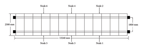
The experiments were conducted on the HUMVIB footbridge situated within the Campus Lichtwiese of TU Darmstadt in Germany. This bridge is a composite (steel–concrete) structure with a span length of 13.24 m. It is built of a pair of longitudinal steel beams with a cross-section of HEB 240. These beams are supported at both ends using articulation. The bridge deck consists of 13 prefabricated concrete slabs resting on these beams (Figure 3(a)). To prevent any shifting of the concrete against the steel, 5mm-thick dummy blocks were strategically placed as separators. It was observed that three such blocks per concrete unit offered greater stability than four. As illustrated in Figure 3(b), these dummy blocks are aligned in alternating orientations for adjacent concrete slabs. Moreover, the bridge’s lateral rigidity has been enhanced by incorporating a crossbeam at three junctures: the start, the middle, and the end of the footbridge. This crossbeam, a U160 × 65 × 7.5 profile, links the main beams via angle steel (L120 × 120 × 12) and bolted joints, as depicted in Figure 3(c). The overview of the chosen footbridge for the laboratory experiments is shown in Figure 3(d).


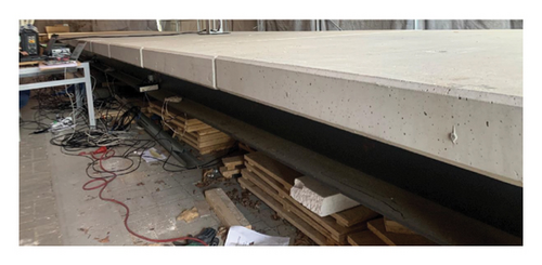
It should be noted that, although equipment appears to be visible under the bridge in Figure 3, all necessary precautions were taken to ensure that no equipment or objects interacted with the structure during the experiments.
3.2. Bridge Instrumentation
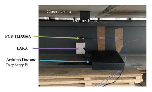
In this study, the bridge was instrumented with an array of sensors consisting of six PCB TLD356A17 accelerometers and six LARA accelerometers. The structure was divided into three equal segments: one at a quarte-span, the midspan, and three-quarters-span. Two nodes were selected within each segment, resulting in a total of six nodes for sensor placement, as depicted in Figure 4(a). Each LARA sensor was positioned adjacent to a PCB sensor, ensuring the longitudinal (X) axis of all sensors was uniformly aligned. The setup of the sensors on the bridge, featuring both a PCB TLD356A17 and a LARA accelerometer, is illustrated in Figure 4(b).
In addition, for clarification throughout this paper, the sensors are identified according to their node location on the bridge. For instance, LARA1 and PCB1 refer to the low-cost and commercial sensors situated at Node 1, respectively.
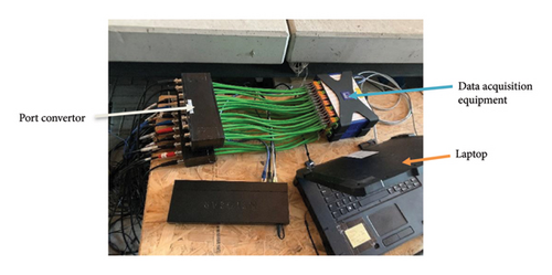
It is important to note the differences in the instrumentation process. While each LARA operates autonomously, the PCB accelerometers require a data acquisition system connected to a computer for data streaming and storage, as demonstrated in Figure 4(b). In contrast, the LARA accelerometers offer a more time-efficient solution, negating the need for additional cables, data acquisition equipment, or a computer for operational control. Instead, they execute preprogrammed instructions via a modifiable Python script, which simplifies the setup process, as shown in Figure 2.
3.3. Bridge Excitation Methodology
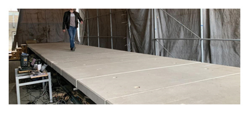
The bridge was subjected to dynamic excitation by a person walking across it. To mitigate the variability in pedestrian excitation, the walking speed was set to approximately 2 Hz using a pendulum as a guiding mechanism. The pendulum helped pedestrians maintain a steady pace, ensuring consistency in the excitation frequency. The chosen speed of 2 Hz aligns closely with the first eigenfrequency of the bridge, thereby enhancing the excitation of the bridge’s dynamic response. This controlled excitation not only improves data consistency but also facilitates the identification of additional mode shapes by resonating with the bridge’s natural frequencies. The action of walking was systematically repeated three times to ensure consistency. In each instance, the individual traversed the bridge from the left to the right abutment, maintaining the target frequency of 2 Hz. Subsequently, the bridge was allowed to freely oscillate for 2 min to observe its natural response. This procedure was precisely replicated at intervals of 0, 3, and 6 min.
The simplicity of the experimental setup was intentional, with conditions controlled to remain as consistent as possible. It is crucial to acknowledge, as illustrated in Figure 5, that despite the aim for uniformity in the walking frequency, there was an element of human variability. These variations, rather than solely posing as a limitation, served a dual purpose. They prevented the AI tool employed for processing LARA’s data from potential overfitting, thereby enhancing the robustness of the study’s findings.
After completing the experiment and extracting data from the data acquisition systems of both PCB and LARA sensors, a postprocessing step was initiated to align the Z-axis and Y-axis data. This alignment ensured a comprehensive analysis of the bridge’s response by standardizing the orientation across all axes and sensors.
Subsequently, the datasets underwent synchronization and were resampled to a uniform sampling frequency of 333 Hz. This frequency was selected based on the maximum sampling capability of the LARA sensors, necessitating the resampling of the PCB sensor data, which was originally collected at 600 Hz, to match.
Upon completing the alignment, synchronization, and standardization of the sampling frequency, data for the Z, X, and Y axes were thoroughly extracted. Given the simply supported nature of the footbridge’s structural design, the analysis primarily concentrated on the Z-axis data. This focus was deliberately chosen to test the training model’s proficiency in refining LARA sensor data to ILARA data. The goal was to ascertain the model’s impact on enhancing data reliability and accuracy for SHM applications. Figure 6 displays the time-domain output from the three PCB sensors used for the training of ILARA.
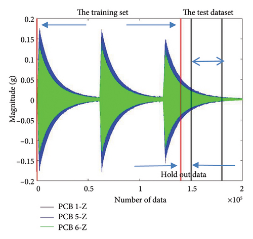
While standard practices often advocate for a fixed percentage split (e.g., 60-20-20), the availability of a large dataset in this study enabled the prioritization of comprehensive training, ensuring the model’s effectiveness in real-life conditions rather than merely in a laboratory setting. A broader range of training data was adopted to enhance the model’s robustness beyond controlled environments, rather than strictly adhering to regions most compatible with the test datasets. This decision was driven by the necessity of replicating real-world scenarios, where data quality varies due to sensor accuracy and imposed loads. By incorporating a diverse dataset, the LSTM model was trained to handle fluctuations and imperfections present in practical applications, such as monitoring an operational bridge using ILARA sensors. In addition, this approach minimized overfitting, improving the model’s ability to generalize when applied to new datasets.
3.4. Architecture of the AI Tool
This subsection illustrates the design and operational mechanics of the LSTM model tailored for analyzing SHM data derived from bridge sensors. The model is trained on the training dataset, and hyperparameters are optimized using the hold-out cross-validation dataset. Finally, the test dataset is used to evaluate the model’s ability to generalize to new data. This thorough process confirms the reliability of the model and ensures it avoids overfitting to the training data. The core of our deep learning strategy involved training the LSTM model to discern complex temporal relationships within the bridge’s dynamic response data, a crucial step towards enhancing the predictive accuracy of low-cost sensor data. It is essential to emphasize that the role of the commercial accelerometer in this study is to validate the proper calibration of LARA readings during the training of the proposed LSTM. The calibration process leverages the LSTM model to address the unique noise characteristics of low-cost accelerometers. By combining data from all available sensors, the model estimates the output of each LARA sensor (e.g., Sensor number 1) and compares this prediction with the sensor’s actual readings and historical data stored in its memory. As a RNN, the LSTM processes data in sequences, incorporating temporal dependencies to refine predictions. This allows the model to account for both spatial relationships among sensors and temporal patterns in the data, effectively identifying and reducing noise.
Unlike traditional calibration methods for commercial sensors, which often rely on linear transformations or static correction factors, the LSTM model dynamically adjusts based on the context provided by prior and concurrent measurements. While the LSTM model functions as a “black box,” limiting the interpretability of its internal mechanisms, its ability to extract meaningful patterns and reduce noise has been validated through experimental results. This trade-off between interpretability and performance is a common characteristic of advanced machine learning models and does not diminish the practical utility of the approach.
It should be noted that overfitting was mitigated by dividing the data into three distinct datasets: a training dataset, a hold-out cross-validation dataset, and a test dataset. The model was trained on the training dataset, and hyperparameters were optimized based on the performance on the hold-out cross-validation dataset. Finally, the model’s generalization ability was evaluated using the test dataset. This process ensured that the model did not overfit the training data, thereby maintaining reliability and robustness when applied to unseen data. By separating these datasets and following this rigorous validation strategy, the model’s performance and generalization capabilities were effectively validated.
The monitoring data are divided into two distinct sets: (1) the training set, comprising the first 140,000 records of the data, (2) the hold-out cross-validation dataset, between 140,000 and 1,500,000, and (3) the test dataset, representing the remaining data from 150,000 to 180,000 records. The hyperparameters are determined through an experimental analysis of the model performance using hold-out cross-validation datasets. A crucial preprocessing step involved standardizing the input features via the “StandardScaler,” ensuring a consistent scale across the diverse dataset. This preparation was vital for the LSTM network to effectively process and learn from the temporal sequences.
The selected architecture for the LSTM model included six input neurons, which encompassed LARA sensors at Nodes 1, 4, and 5, in conjunction with PCB sensors at Nodes 2, 3, and 6 as can be seen in Figure 3(a). This unique combination of input data, spanning across different sensor types and locations, is chosen to encapsulate a broad spectrum of the bridge’s dynamic behavior. The training dataset, aimed at guiding the model’s learning process, comprised the responses from PCB sensors 1, 4, and 5 in its output layer. This selection was instrumental in refining the model’s ability to accurately predict the bridge’s dynamic characteristics, underpinned by the high-quality measurements provided by these specific PCB sensors. For the test dataset, the output dataset is represented as ILARA outputs which are enhanced versions of LARA measurement for Nodes 1, 4, and 5. The model’s architecture is designed with a sequence of three LSTM layers, each consisting of 30 units and one feed-forward layer. Figure 7 shows the models’ architecture.

The ReLU activation function is used in LSTM layers. The model variables for the considered LSTM are listed in Table 2.
| Initial learning rate | 0.001 |
| Epochs | 50 |
| Number of hidden layers | 4 |
| Units | 30 |
| Activation function | ReLU |
| Solver | Adam |
| Normalizer feature | StandardScaler |
| Loss function | Mean squared error |
| Time step | 5 |
The resultant ILARA output, which indicates the model’s enhanced data acquisition capabilities, represents a significant improvement in the quality of insights derived from LARA sensors. This effort to leverage deep learning to enhance SHM data quality through LARA sensors, while strategically integrating PCB sensor data for model training, signifies a major advancement. It not only increases the feasibility of using fewer high-cost PCB sensors across extensive bridge networks but also moves us toward a more cost-effective and reliable approach to SHM.
Figure 8 presents a series of scatter plots that compare PCB accelerometer measurements (horizontal axis) with two types of LARA sensor outputs (vertical axis). Each row corresponds to a specific sensor node on the bridge: the left plot in each row displays raw LARA data (i.e., uncalibrated) versus PCB, while the right plot shows ILARA data (i.e., calibrated via the LSTM model) versus PCB. Every individual point on the plots represents a paired measurement from the PCB and LARA sensors. The red dashed line (y = x) indicates where the two measurements would be in perfect agreement. Comparing the left and right columns reveals that the calibrated ILARA data exhibit improved alignment with the PCB measurements, illustrating the effectiveness of the proposed LSTM–based calibration approach in reducing noise and enhancing measurement accuracy.
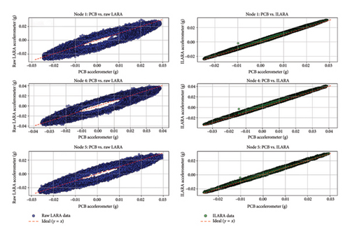
The analysis of the scatter plots in Figure 8 reveals a clear improvement in data accuracy achieved through the ILARA calibration process. In the left column, which compares PCB reference data with raw LARA measurements, there is noticeable scatter indicating inconsistencies and lower precision in the raw LARA data relative to the PCB sensor. In contrast, the right column shows that the ILARA data are more closely aligned with the ideal (y = x) line, signifying enhanced consistency and accuracy after calibration.
To quantify the signal recovery capabilities of the LSTM–based network, a detailed error analysis was conducted, comparing the raw LARA sensor data and the enhanced ILARA data against the reference PCB sensors. The mean squared error (MSE), root MSE (RMSE), and mean absolute error (MAE) were computed for each monitored node to provide a localized assessment of the corrections achieved by the LSTM–based model. The results presented in Table 3 illustrate a significant reduction in error across all nodes, demonstrating the effectiveness of the proposed AI–driven calibration approach.
| Node | Metric | LARA vs. PCB | ILARA vs. PCB |
|---|---|---|---|
| Node 1 | MSE | 3.1209 × 10⁻⁴ | 3.0185 × 10⁻⁶ |
| RMSE | 0.01767 | 0.00174 | |
| MAE | 0.01367 | 0.00158 | |
| Node 4 | MSE | 5.7875 × 10⁻⁴ | 6.7069 × 10⁻⁶ |
| RMSE | 0.02406 | 0.00259 | |
| MAE | 0.01863 | 0.00235 | |
| Node 5 | MSE | 3.1766 × 10⁻⁴ | 1.7942 × 10⁻⁶ |
| RMSE | 0.01782 | 0.00134 | |
| MAE | 0.01379 | 0.00112 | |
The analysis of Table 3 shows that, compared to the uncorrected LARA data, the ILARA outputs exhibit a substantial decrease in MSE, RMSE, and MAE at each node. Overall, these results demonstrate that the current ILARA calibration approach is effective to a certain extent. However, the exact scope of these improvements can only be determined through a subsequent modal analysis, which will help identify which signal components are most improved and uncover any previously hidden mode shapes now discernible in the calibrated data.
It should be noted that the application of AI to low-cost sensors is a relatively novel approach, and this study represents an early attempt to validate its feasibility. Currently, the LSTM model must be trained specifically for each bridge to account for its unique characteristics and conditions. Although the results presented here are case-specific, they provide a foundation for broader applications and demonstrate the potential of this methodology in SHM.
Future research will focus on enhancing the scalability and versatility of this approach by optimizing the methodology for bridges with varying structural characteristics. One promising direction is the use of transfer learning, which would allow a model trained on one bridge to be adapted to another with minimal additional training. This advancement could significantly reduce the need for extensive retraining, improving both the practicality and generalizability of the proposed method.
The bridge selected for this study was chosen due to its specific structural conditions, which provided an ideal setting to validate the methodology under controlled circumstances. The complexity of the selected bridge also underscores the robustness of the proposed model in handling challenging structural dynamics. In addition, the algorithm’s reliance on temporal calibration of low-cost sensors using commercial ones makes it inherently adaptable to other systems. Such calibration can be seamlessly integrated into standard bridge inspection protocols. For newly constructed bridges, calibration aligns naturally with mandatory static and dynamic load tests often required by regulatory standards. For older bridges, it can be incorporated into scheduled dynamic load tests using temporary instrumentation, ensuring compatibility with existing maintenance practices and maximizing the utility of the proposed system.
4. Comparative Analysis of Modal Value Estimations of LARA, PCB, and ILARA
In this section, an analysis is conducted on the data acquired from LARA and PCB sensors, as well as the data enhanced to ILARA, using an OMA approach. Among various OMA methodologies, the frequency domain decomposition (FDD) method is employed, utilizing a widely accessible FDD MATLAB code found online. This approach was selected to simplify the process and avoid the necessity for complex and costly OMA analysis tools such as Artemis software. The FDD method, a frequency-based approach, was chosen for its ease of use and its applicability in evaluating the modal values through a frequency domain application, given the ILARA data had been trained in the time domain. This decision highlights the objectives of simplicity and rigorous evaluation of ILARA’s frequency domain capabilities.
4.1. Eigenfrequencies and Mode Shapes From PCB Sensors
This subsection presents the FDD [87] analysis, conducted using Z-axis data from PCB sensors.
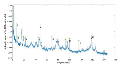
Figure 9 illustrates the selected tips for the FDD analysis based on data from PCB sensors at Nodes 1, 4, and 5 (Figures 3(a)).
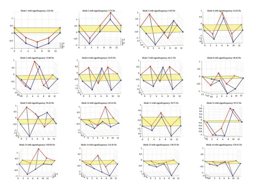
To gain deeper insights into the mode shapes of the bridge, additional modal analysis was performed using data from PCB sensors located across Nodes 1 through 6. The comprehensive dataset from all nodes facilitated the creation of Figure 10, which displays the bridge’s mode shapes for the first 16 modes.
4.2. FDD Analysis of LARA Sensors Data
In this subsection, attention is turned towards the modal value estimations derived from the LARA sensors, employing the FDD methodology consistent with the preceding analysis. Figure 11 displays selected tips for the FDD analysis based on data from LARA sensors at Nodes 1, 4, and 5.
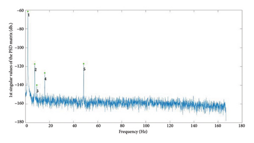
The comparative analysis between Figures 9 and 11 highlights the differences in accuracy and resolution between LARA sensors and PCB sensors. It is evident that while PCB sensors detected more than 16 modes, LARA sensors identified only 5 tips. It is important to note that an equal amount of data from both LARA and PCB sensors was used for this analysis. In addition, the sampling frequencies of both systems have been synchronized. Considering these measures, the difference in resolution between the LARA sensors and the commercial PCB sensors is clearly demonstrated by analyzing Figures 9 and 11.
4.3. Insights From ILARA–Enhanced Data
In this subsection, an examination is conducted on the impact of LSTM processing on enhancing the data quality of ILARA sensors, specifically regarding the accuracy and reliability of modal value estimations. Observations on improvements or discrepancies when compared to LARA and PCB sensors’ data are highlighted, illustrating the benefits and limitations of the LSTM enhancement process.
Figure 12 displays selected tips from an FDD analysis on the ILARA–enhanced data.
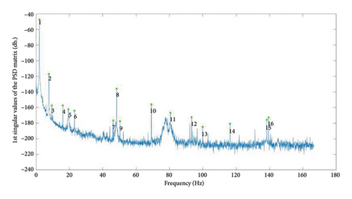
The analysis of Figure 12 indicates that the accuracy of ILARA’s enhanced data has improved, although it raises concerns as the tips and the shape of the FDD closely resemble those in Figure 9. This similarity may be due to the LSTM model’s configuration, which includes six input neurons from LARA sensors at Nodes 1, 4, and 5, combined with PCB sensors at Nodes 2, 3, and 6. This strategic combination has led to better identification in the eigenfrequency analysis of the bridge. However, it is important to note that the chosen PCB nodes within the input neurons were not adjacent to the LARA nodes.
4.4. Comparative Evaluation of Modal Value Estimations
This subsection presents a comprehensive comparison of the modal values obtained from PCB, LARA, and ILARA datasets. The analysis begins by comparing the modal values of the different systems, calculating their differences relative to those of PCB sensors. The mode shapes of different systems have been also compared with each other in this subsection using the modal assurance criterion (MAC) [88] value. The MAC value is a statistical measure that quantifies the similarity between two mode shapes, ranging from 0 to 1. A value of 1 indicates identical mode shapes, while a value closer to 0 suggests a greater discrepancy [89].
Table 4 compares the modal estimations of PCB sensors with the data from LARA.
| Mode number | Frequency PCB (Hz) | Mode shapes PCB | Mode shapes LARA | Freq (%) | MAC Z | ||||
|---|---|---|---|---|---|---|---|---|---|
| Node 1 | Node 4 | Node 5 | Node 1 | Node 4 | Node 5 | ||||
| 1 | 2.032 | −0.733 | −1.000 | −0.747 | −0.731 | −1.000 | −0.727 | 0.000 | 1.000 |
| 2 | 7.723 | −0.980 | 0.010 | 1.000 | −1.000 | −0.069 | 0.975 | 0.524 | 0.996 |
| 3 | 9.471 | −0.970 | 0.081 | 1.000 | −0.909 | −0.434 | 1.000 | 0.000 | 0.869 |
| 4 | 16.097 | −0.675 | 1.000 | −0.688 | −0.607 | 1.000 | −0.612 | 0.252 | 0.997 |
| 5 | 19.471 | −0.950 | −1.000 | −0.977 | |||||
| 6 | 23.048 | −0.297 | −1.000 | −0.897 | |||||
| 7 | 46.096 | −0.624 | 0.695 | 1.000 | |||||
| 8 | 48.332 | −0.147 | −0.307 | −1.000 | −0.168 | −0.285 | −1.000 | 0.084 | 0.999 |
Analysis of Table 4 shows that LARA identified only 5 tips in the FDD analysis. However, the modal values measured by LARA sensors are well captured, as evidenced by MAC values near 1 when comparing the mode shapes of LARA (Nodes 1, 4, and 5) with those of PCB sensors (Nodes 1, 4, and 5), demonstrating LARA’s high capability. Nevertheless, due to LARA being a low-cost MEMS accelerometer with higher noise density compared to PCB sensors (Table 1), it was not able to identify more modes.
Table 5 compares the modal estimations of PCB sensors with the enhanced data from ILARA.
| Mode number | Frequency PCB (Hz) | Mode shapes PCB | Mode shapes ILARA | Freq (%) | MAC Z | ||||
|---|---|---|---|---|---|---|---|---|---|
| Node 1 | Node 4 | Node 5 | Node 1 | Node 4 | Node 5 | ||||
| 1 | 2.032 | −0.733 | −1.000 | −0.747 | −0.740 | −1.000 | −0.750 | 0.000 | 1.000 |
| 2 | 7.723 | −0.980 | 0.010 | 1.000 | −0.962 | 0.097 | 1.000 | 0.000 | 0.996 |
| 3 | 9.471 | −0.970 | 0.081 | 1.000 | −0.881 | 0.150 | 1.000 | 0.000 | 0.995 |
| 4 | 16.097 | −0.675 | 1.000 | −0.688 | −0.399 | 1.000 | −0.347 | 0.000 | 0.922 |
| 5 | 19.471 | −0.950 | −1.000 | −0.977 | −0.786 | −1.000 | −0.819 | 0.000 | 0.992 |
| 6 | 23.048 | −0.297 | −1.000 | −0.897 | −0.713 | −1.000 | −0.733 | 0.000 | 0.903 |
| 7 | 46.096 | −0.624 | 0.695 | 1.000 | −1.000 | 0.709 | 0.704 | 0.526 | 0.886 |
| 8 | 48.332 | −0.147 | −0.307 | −1.000 | −0.700 | −1.000 | −0.700 | 0.000 | 0.008 |
| 9 | 50.365 | −0.881 | −0.647 | 1.000 | −0.527 | 1.000 | −0.122 | 0.000 | 0.033 |
| 10 | 69.185 | −0.716 | −1.000 | 0.595 | −0.240 | −1.000 | 0.333 | 0.059 | 0.860 |
| 11 | 78.901 | −0.293 | 0.119 | 1.000 | −0.174 | −1.000 | 0.269 | 2.118 | 0.033 |
| 12 | 93.290 | −1.000 | −0.591 | 0.926 | −0.122 | 1.000 | −0.068 | 0.000 | 0.126 |
| 13 | 99.957 | −0.828 | 1.000 | 0.078 | −0.227 | −1.000 | 0.273 | 0.041 | 0.328 |
| 14 | 116.339 | −0.368 | 0.421 | −1.000 | −0.142 | −1.000 | 0.220 | 0.000 | 0.247 |
| 15 | 138.330 | −0.205 | −0.263 | −1.000 | −0.063 | 1.000 | −0.245 | 0.000 | 0.000 |
| 16 | 139.427 | −0.155 | 0.138 | −1.000 | −0.091 | 1.000 | −0.314 | 0.000 | 0.188 |
- Note: Bold values show a MAC value below 0.8, indicating a lack of correlation between the mode shapes detected by the LARA system and those measured by the PCB sensors.
Analysis of Table 5 indicates that ILARA performed a better eigenfrequency analysis than LARA, marking an important improvement. It is also noted that ILARA identified 7 modes, six of which have a MAC value over 0.9. This high accuracy can be considered a significant step towards utilizing AI to enhance the modal analysis of low-cost sensors. However, the analysis also reveals that for higher mode numbers, the MAC values were insufficient. It is proposed that with more complex training, such as using a shaker to excite the bridge or conducting more experiments on the bridge under study, the training of ILARA could be enhanced, potentially resulting in a better system. This paper, for the first time in the literature, attempts to improve the modal analysis of low-cost sensors by combining the acquired data of low-cost and commercial sensors, which may pave the way for future improvements and advancements.
Figure 13 visualizes and compares the frequencies and MAC between PCB sensors and two sensor types: with data coming from LARA (Table 4) and ILARA (Table 5).
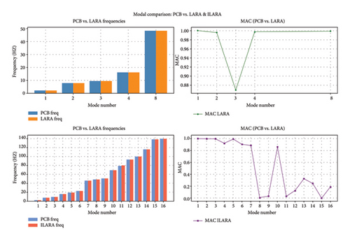
The bar chart on the top left of the figure compares the eigenfrequency values measured by PCB sensors with those computed for LARA. The results show minimal differences between PCB and LARA eigenfrequencies for most modes, confirming the consistency of measurements between the two systems. However, it is evident that eigenfrequencies for Modes 5–7 are unavailable, indicating gaps in LARA’s ability to detect certain higher-order frequencies. Despite this limitation, the available frequencies exhibit strong agreement.
The chart on the top right illustrates the MAC values for PCB and LARA mode shapes. MAC values close to 1.0 (100%) indicate excellent correlation, and in this Figure 13, all modes analyzed (Modes 1–3 and Mode 8) have MAC values above 0.85, reflecting strong alignment between PCB and LARA mode shapes.
The bar chart on the bottom left of the Figure 13 compares the eigenfrequency values measured by PCB sensors with those computed for ILARA. ILARA demonstrates the capability to identify up to 16 modes of eigenfrequencies, with a generally strong agreement between the two systems.
The chart on the bottom right illustrates the MAC values for PCB and ILARA mode shapes. The results are more variable compared to LARA. Modes 1–7 and Mode 10 exhibit MAC values above 0.9, indicating strong correlations. However, Modes 8, 9, 11, and 15 exhibit lower MAC values, suggesting less similarity between the mode shapes detected by ILARA and PCB. This variability highlights the challenge of detecting higher mode shapes accurately. While eigenfrequency detection remains relatively straightforward, mode shape detection for higher modes is more sensitive to noise and requires advanced noise cancellation and data correction techniques. The algorithm proposed in this paper aims to minimize data postprocessing and relies on a consistent OMA code applied to both systems, demonstrating reliable performance within these constraints.
In the context of bridge maintenance and OMA, the first mode or the first three mode shapes are typically prioritized, as they provide critical insights into the global behavior of the structure. Higher modes are often excluded from practical analyses due to their sensitivity to noise and limited relevance in standard maintenance protocols. The LARA system, by itself, can accurately identify up to the first four mode shapes. However, with the implementation of the proposed algorithm, the ILARA system extends this capability to reliably analyze up to the first seven mode shapes. This performance is more than sufficient for most OMA tests in civil engineering, ensuring that the system effectively meets the demands of SHM while maintaining simplicity and computational efficiency.
5. Conclusions
SHM plays a pivotal role in ensuring the integrity and safety of vital infrastructure, such as bridges. Despite its importance, the widespread adoption of SHM is often hindered by the high costs associated with traditional sensors. This study introduces an innovative approach that seeks to expand SHM capabilities by integrating low-cost MEMS accelerometers with high-accuracy commercial sensors through a deep learning framework based on LSTM neural networks.
While low-cost MEMS accelerometers offer a more economical alternative, they typically face challenges regarding accuracy and resolution when compared to their commercial counterparts. Addressing these challenges, this research has developed a novel method to calibrate and refine the accuracy of data acquisition from these economical devices. This is particularly significant as the domain of SHM becomes increasingly complex, underscoring the need to efficiently utilize low-cost sensors without degrading the quality of data.
It is important to note that the main objective of this study is not to replace commercial sensors entirely with enhanced low-cost ones but rather to reduce the dependency on expensive commercial sensors by 50%. This reduction aims to maintain an acceptable flow of data while substituting some high-cost sensors with calibrated low-cost alternatives, thereby significantly reducing the overall budget required for SHM systems.
The LSTM model employed in this study has demonstrated that low-cost sensors, when augmented with AI, can serve as a viable alternative to more expensive commercial sensor systems, ensuring data quality and accuracy are upheld. However, to further enhance and verify this method, additional experiments employing various excitation methods are recommended. Future research will focus on continuing to refine these techniques, broadening the applicability and reliability of low-cost sensors in SHM and exploring the potential for greater cost reductions across broader infrastructure networks.
It should be noted that while the ILARA system represents significant progress in cost-effective SHM, certain limitations must be addressed. The current methodology relies on the temporal calibration of low-cost sensors using commercial ones during dynamic load tests. Although this calibration process can be seamlessly integrated into standard bridge testing protocols, such as mandatory static and dynamic load tests for newly constructed bridges or periodic dynamic tests for older bridges, it introduces practical barriers for widespread adoption due to the need for temporary instrumentation.
Future investigations will focus on adapting and optimizing the methodology for bridges with varying structural characteristics to improve its versatility and scalability. A key direction is the exploration of transfer learning, enabling a model trained on one bridge to be adapted and applied to another bridge with minimal additional training. This advancement would significantly enhance the generalizability and practicality of the method, reducing the need for extensive retraining for each new case.
In addition, the system’s validation has been conducted on a limited number of structures, requiring further experimental tests on a wider range of structural systems and under diverse conditions to ensure robustness and generalizability. Long-term monitoring and testing under varying excitation methods, including calibrating the system with one excitation and verifying its performance under another, should also be explored. These steps are essential to refine the methodology, improve its scalability, and reduce its dependency on commercial sensors for calibration, thereby enhancing its practicality and adoption potential.
Conflicts of Interest
The authors declare no conflicts of interest.
Author Contributions
Seyyedbehrad Emadi, Seyedmilad Komarizadehasl, and Ye Xia conceived and designed the research. Seyyedbehrad Emadi developed the algorithm, performed the model training, and conducted the evaluations. Seyedmilad Komarizadehasl provided the experimental data, assessed the trained models, and quantified and interpreted the improvements. Ye Xia contributed to data visualization, edited the manuscript, assisted with writing, and helped organize the manuscript. Seyedmilad Komarizadehasl served as the corresponding author, facilitating collaboration between Seyyedbehrad Emadi and Ye Xia and providing all necessary materials and data for the study.
Funding
The authors extend their sincere gratitude for the support provided by the projects PID2021-126405OB-C31, funded by FEDER funds, A Way to Make Europe and Spanish Ministry of Economy and Competitiveness MICIN/AEI/10.13039/501100011033/. Furthermore, the research benefited from a grant bestowed by the Universitat Politècnica de Catalunya, identified as ALECTORS-2023, under the leadership of Dr. Komarizadehasl. This study was also supported by the National Natural Science Foundation of China (52278313 and 52411540031).
Open Research
Data Availability Statement
The data supporting the findings of this study are available upon reasonable request. Due to privacy concerns and proprietary restrictions, access to the data may be granted on a case-by-case basis. Interested researchers may contact the corresponding author for further details.


