Zero-shot learning approaches have emerged as promising techniques for structural health monitoring (SHM) due to their ability to learn representations without labeled data. With the practical design of such models, the shift from traditional structure-dependent techniques to potentially large-scale implementations becomes feasible, effectively addressing the challenge of gathering labeled data. Autoencoders (AEs), a class of deep neural networks, align well with zero-shot SHM settings due to their architecture, loss function, and optimization process. In AEs, the reconstruction error is expected to increase for novel data patterns (i.e., potential damage data), while the encoded manifold in their bottleneck layers enables the discrimination of complex patterns. However, for practical SHM applications, rigorous evaluation of (variational) AEs and the robustness of reconstruction loss- or manifold-based designs in handling real-world scenarios remains necessary. Accordingly, this article employs two SHM benchmarks to evaluate the effectiveness of manifold learning compared to the reconstruction errors of (variational) AEs in a zero-shot setting. The comparison encompasses metrics such as reconstruction fidelity, preservation of structural characteristics, and the ability to generalize to unseen structural conditions. Furthermore, an unbiased normalization-based ensemble methodology is proposed, combining both approaches with the goal of enhancing damage detection performance and delivering more reliable results in zero-shot learning contexts. The proposed ensemble strategy, integrating both reconstruction error and manifold representations, adds robustness to the damage detection process, a crucial feature in the uncertain domain of zero-shot structural damage detection. The findings suggest that neither reconstruction loss nor manifold data consistently outperform the other; structural differences may render one approach more effective than the other in specific contexts, and based on these observations, a zero-shot damage severity index is suggested and tested on the benchmark data. Nevertheless, the proposed ensemble method demonstrates superior performance over individual models in estimating damage severity in an unsupervised setting. These results highlight the efficacy of variational AEs for zero-shot SHM, offering insights into their strengths and limitations and aiding users in selecting appropriate zero-shot damage detection strategies in the absence of labeled data.

1. Introduction

Structural health monitoring (SHM) is an umbrella term that encompasses various techniques and procedures, including structural damage detection (SDD), which provides a framework for ensuring the safety and longevity of critical infrastructure. Timely damage detection and prognosis are essential for tracking undesired changes in structural characteristics over time, assessing the overall condition of a structure, and determining whether it can continue to perform its intended functions. In this context, SHM is employed to prevent further deterioration by conducting routine structural assessments across civil, mechanical, and aerospace engineering [1–3].

SHM frameworks encompass both model-based and data-driven approaches. The model-based strategy relies on a “model” constructed from known structural design details, such as specifications for beams and columns (e.g., [4]), which can be coupled with techniques such as inverse problem methods to further calibrate (“tune”) these numerical models (e.g., finite element models). Through the parallel numerical model, various SHM objectives, including SDD, can be performed [5–7]. The data-driven approach involves monitoring the system’s behavior over time by analyzing the dynamic or vibration responses of the structure, particularly the acceleration data collected from a group of channels (sensors) [1].

The data-driven method is characterized by the identification and interpretation of underlying data patterns that can be linked to various structural states or conditions of interest. Still, the two methods may overlap, particularly with the advent of surrogate modeling and data-driven model updating, both of which can be achieved using deep learning (DL) techniques (e.g., [8]), or statistical methods (e.g., [9]). Statistical pattern recognition and machine learning (ML) remain classical and widely adopted means for implementing data-driven SHM frameworks [3, 10, 11].

Using the aforementioned model, the damage detection process generally involves two main components: feature extraction and feature classification [12, 13]. The inherent nonlinearity and noise present in SHM data, coupled with the limitations of traditional models in discerning patterns within such data, make the feature selection step particularly challenging. As a result, this step is often guided by expert judgment and trial-and-error procedures. This challenge is well-documented in the literature (e.g., [11, 14–17]), where feature extraction is frequently highlighted as a critical phase. Feature selection through wavelet (packet) transforms and the Hilbert–Huang transform [18–22], known for their ability to capture damage-sensitive characteristics, have become established methods for feature extraction. Similarly, time-series modeling [12] has been used to extract and examine changes in structure responses with damage-sensitive feature (DSF) extraction, even on environmental and operational variations (EOVs) [14]. These features are derived mainly directly or indirectly from the coefficient and residuals of the time-series model [14, 23–26]. In the realm of feature classification, artificial neural networks (ANNs) [27] and support vector machines (SVMs) [28] are commonly acknowledged as capable feature classifiers.

Still, feature selection can become a bottleneck in developing generalizable SHM solutions. SHM performance heavily relies on the quality of the extracted features, which domain experts need to carry out for feature selection, a case-dependent process. Moreover, as feature extraction and damage classification are distinct procedures, the features obtained may not be ideal for classification purposes. However, DL has emerged as a comprehensive modeling approach capable of addressing these limitations [29]. DL models operate through representation learning, in which both feature extraction and the target task (e.g., classification) are jointly optimized.

In SHM, supervised learning refers to cases where data on both healthy and damaged conditions are available [29, 30], while unsupervised learning is applied when labels are not used during training [31, 32]. Although supervised learning has demonstrated remarkable performance, it presents significant challenges in real-world applications, particularly due to the difficulty in collecting labeled data from actual structures [33]. In contrast to supervised learning, unsupervised learning algorithms do not depend on data labels but instead learn implicit patterns directly from the data [34]. These methods, such as representation learning, density estimation, and cluster analysis, enable the discovery of the underlying patterns and relationships in unlabeled data to support informed decisions without needing labeled data [35, 36]. However, the ability of unsupervised approaches to distinguish between different damage classes remains underdeveloped [36]. Additional concerns include the curse of dimensionality, which refers to the exponential increase in data complexity with rising feature dimensions [37] and the presence of noise and outliers in the data, which can adversely affect the accuracy of unsupervised learning, remain as significant concerns. Ultimately, even though unsupervised methods are needless of labels, both damage and no-damage data are needed unless the zero-shot approach is pursued.

These challenges underscore the need for robust and efficient zero-shot unsupervised learning algorithms capable of handling high-dimensional data, accounting for noise and outliers, and capturing complex patterns and relationships, even in the absence of historical structural data. In the context of damage detection, unsupervised learning methods have been applied to tasks such as damage identification and classification [38]. Deep unsupervised learning has further enhanced the performance of traditional unsupervised ML models [39–47], while also enabling the reconstruction of missing data in SHM systems [48]. Nevertheless, employing DL models to zero-shot damage diagnosis remains relatively limited and is still an emerging area of research [44].

Zero-shot SDD presents a significant challenge in SHM, as it involves identifying structural damage without prior knowledge of how such damage affects structural behavior [49–51]. In the absence of labeled data, zero-shot learning relies on innovative loss functions and heuristics to produce reliable outcomes for previously unseen data classes, in this case, damaged structural states. When considering a simple binary classification between “damaged” and “undamaged” conditions, where the model is never exposed to damaged data during training, autoencoders (AEs) emerge as a promising solution. Owing to their architecture, AEs are well-suited for anomaly detection through two principal strategies: utilizing reconstruction error (RE) and analyzing manifold representations (i.e., encoder outputs). Most existing studies emphasize the first strategy, RE, to detect damage [42, 52–55], or employ reconstruction-based data normalization [56]. However, the manifold data can also be leveraged in various semisupervised and unsupervised learning approaches, commonly referred to as manifold learning [57–59]. Manifold learning is an algorithm for reducing the dimensionality of data from high-dimensional to low-dimensional spaces. As with the anticipated higher reconstruction loss error for future damage scenarios, the different projections of the input data into the low-dimensional space can capture the differences in incoming unseen damage data from the structure’s baseline condition.

To summarize, various ML and DL models have been applied to SDD, covering a range of supervision levels in the literature. These studies highlight the strengths and limitations of different strategies and architectures. However, limited research has specifically focused on zero-shot SDD, which represents the least case-dependent approach and holds promise for enabling large-scale SHM applications. Furthermore, even in unsupervised methods, where damage data may be available but unlabeled, advancing from basic damage detection to quantifying damage severity remains a significant challenge.

Accordingly, this study introduces a novel perspective by exploring the potential of zero-shot DL-based SDD through the following objectives:

•
Customize and apply DL-based strategies, specifically variational AE’s (VAE) reconstruction loss and manifold learning, in the zero-shot SDD context.
•
Propose an unbiased normalization-based ensemble approach to address the limitations of relying solely on RE or manifold data, thereby improving the reliability and accuracy of zero-shot learning in SHM for real-world scenarios with unlabeled data.
•
Evaluate the effectiveness and sensitivity of both methods in distinguishing between damage classes, and propose a zero-shot damage severity score, which is successfully applied to benchmark data with incremental damage cases.

The research is structured as follows. Section 2 describes the proposed ensemble methodology and its approach. Section 3 outlines the dataset and preprocessing steps. Section 4 presents experimental results, highlighting performance metrics and comparisons. Finally, Section 5 offers concluding remarks, summarizing key findings and future directions.

2. Methodology

2.1. VAE

A VAE builds upon the traditional AE by introducing a probabilistic framework to the latent space. Instead of mapping inputs to fixed points, the encoder generates a distribution (typically Gaussian). This allows the VAE to capture uncertainty and improve its ability to create diverse and more realistic outputs compared to the deterministic nature of a standard AE [52]. Figure 1 shows the general overview of the VAE network.

Details are in the caption following the image — **Figure 1**
Open in figure viewer PowerPoint

General overview of the VAE network.

Similar to an AE, the VAE architecture consists of two main components: an encoder and a decoder. It aims to learn a compressed representation of the input data unsupervised. The encoder, typically represented by f_enc, maps the input data to a latent space representation z as

()

The decoder, represented by f_dec, reconstructs the input data from this latent representation as

()

During training, the AE minimizes the reconstruction loss, typically defined as the mean squared error (MSE) between the input x and the reconstructed output

, as

()

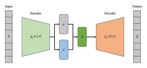
The objective is to learn a latent representation z that captures essential features of the input data, effectively compressing it and enabling the reconstruction of the original input with minimal loss.

The VAE extends the AE’s concept, introducing a probabilistic interpretation of the latent space [53]. It involves learning the parameters of a probability distribution that generates latent representations. The encoder in a VAE maps the input data to the parameters of a probability distribution q(z|x), where the latent variable z is modeled as a Gaussian distribution with mean μ(x) and standard deviation σ(x) as

()

The latent variable z is sampled from this distribution, reparametrized as

()

where ϵ is sampled from a unit Gaussian distribution. The decoder then reconstructs the input data from this sampled latent variable as p_θ(x|x).

The VAE optimizes a loss function comprising two terms, including the reconstruction loss, similar to the AE, and a regularization term based on the Kullback–Leibler (KL) divergence between the learned distribution q(z|x) and the prior distribution p(z) (usually a unit Gaussian) as

()

The VAE’s objective is to reconstruct the input data and ensure that the learned latent space follows a predefined distribution, enabling structured and continuous representations in the latent space.

2.2. Network Architecture

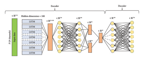
Figure 2 demonstrates a VAE architecture used for the comparison in this article. The encoder encodes the input data into a low-dimensional feature space, from which the input data are reconstructed. Accordingly, the neural network layer that better understands the input vibrational data and generalizes it to unseen data variations is needed. Previous research studies [44] have shown the potential of recurrent neural networks (RNNs), and more specifically, the long short–term memory (LSTM) units, to extract generalizable features from such input data. The VAE encoder part is thus designated with the channel-based LSTM architecture, and the decoder is followed by fully connected layers up to the input size. Figure 2, shows the VAE architecture used in this study.

2.3. Reconstruction and Manifold Learning Approaches in VAE

Based on the VAE outputs, two approaches exist for damage detection. In the first approach, the reconstruction data of each network are used, and in the second approach, the manifold data (i.e., the output of the encoder) can be used through manifold learning.

2.3.1. RE

The RE in VAE is an effective diagnostic indicator since the model approximation of the input is expected to be higher for damaged data, since they deviate more from the normal data with which the network was tuned. The network is trained using a segment of data, which are assumed to represent the baseline or undamaged state (i.e., zero-shot training). Subsequently, the system transitions to a testing phase, during which it evaluates the damage status of new incoming data employing the reconstruction loss of the incoming data. This paper establishes a probability network model for further quantifying damage severity based on the RE. The potential diagnostic mechanisms will be discussed and rigorously examined through the experiments provided in the results section. This feature, the mean square error between reconstructed data and input data, can be obtained as follows:

()

2.3.2. Manifold Learning

SHM often faces significant challenges due to the complex, high-dimensional nature of the data, which complicate data modeling and the monitoring of internal structural changes. To address these complexities, dimensionality reduction offers an effective method for preprocessing high-dimensional datasets. Manifold learning re-represents high-dimensional data within a low-dimensional space, similar to the traditional dimension reduction techniques. In ML, this technique operates on the assumption that high-dimensional data typically lie near specific low-dimensional manifolds [57].

One novel aspect of this research is the application of VAE in manifold learning [54]. Manifold learning seeks to capture data’s intrinsic patterns and relationships by representing them in a lower-dimensional space, providing a more compact yet insightful understanding of complex structural behavior. This study explores how VAEs capture the underlying manifold of structural data within their latent spaces.

The VAE attempts to compress and map the key features necessary for data reconstruction into a low-dimensional space with its deterministic framework. This capability becomes particularly crucial in SHM, where accurately detecting structural damage depends on understanding subtle variations within the underlying manifold of the data. The probabilistic nature of the VAE allows it to better account for uncertainties, which is particularly beneficial for anomaly detection in real-world applications where damage scenarios may be complex and variable.

In our work, the VAE manifold data are leveraged to examine the high-dimensional features extracted through ML models, particularly in the context of zero-shot learning. Here, the encoder output from the VAE models is obtained to capture the reduced, low-dimensional representations of the structural data as

()

This lower-dimensional representation z, produced by the encoder, serves as the key feature set for downstream anomaly detection tasks. The VAE encoder’s output is utilized as a dimensionality reduction module, effectively compressing the input into a latent space that captures the essential structural characteristics.

To perform anomaly detection in a zero-shot learning context, where only the no-damage data are available for training, the OCSVM algorithm is employed. SVMs are known for two core capabilities that work in tandem: first, data are mapped into a high-dimensional space using a kernel function; second, an optimal hyperplane is determined to maximize the margin between data classes. The support vectors, data points closest to the decision boundary, define this margin, ensuring robust separation [55]. One-Class SVM (OCSVM), a variant designed for anomaly detection, learns a decision boundary around the majority class (typically labeled as “normal,” e.g., Label 0) while implicitly treating a small fraction of data as potential outliers (Label 1). The inherent ability of SVMs to create clear class boundaries and maintain margin separation makes them well-suited for SHM and SDD (SHM-SDD), where distinguishing anomalies is essential. The successful application of OCSVM in such contexts has been repeatedly demonstrated in the literature [60]. The OCSVM is trained on the manifold features extracted from the no-damage data (the current condition class) in the bottleneck layer of the VAE. The trained OCSVM then serves as an anomaly detector, flagging any deviations from the learned normal data as potential instances of structural damage [61]. The negative of the OCSVM score (S), which is known as the raw anomaly scores (log-likelihoods), where higher values correspond to greater anomaly for each sample under the fitted model, is performed for the manifold learning SDD base approach. This method effectively utilizes the OCSVM to detect unseen damage scenarios, relying entirely on the manifold representations learned from the undamaged data.

By combining manifold learning with OCSVM for anomaly detection, the proposed approach capitalizes on the strengths of the VAE’s ability to capture and represent the underlying manifold of structural data. This methodology enables robust damage detection in zero-shot learning, providing a promising framework for real-world SHM applications, where acquiring labeled damage data is often impractical or impossible.

2.4. Proposed Unbiased Normalized Ensemble Methodology

This research addresses the challenge of determining whether RE or manifold data from VAE networks are more effective for SDD in zero-shot learning scenarios. Both RE and manifold learning represent critical yet distinct features, but it is not always clear which one yields superior results under varying damage conditions. An unbiased normalized ensemble methodology is proposed to address this uncertainty. The proposed method is designed to facilitate both the RE and the manifold learning to contribute to the final decision. This is achieved by applying z-score normalization to both, standardizing them based on the mean and standard deviation of the no-damage training data. By normalizing the outputs, the method ensures that the contributions of each feature are unbiased, preventing either component from disproportionately influencing the ensemble simply due to differences in their original magnitude or scale.

For the RE component, z-score normalization is performed as follows:

()

where

is the z-score normalized RE for the i-th data point, x_RE,i is the raw RE for the i-th sample, and

and

are the mean and standard deviation of the RE, which are calculated from the no-damage training data. It should be noted that the

refers to the number of data points used for training through zero-shot learning.

Similarly, the manifold learning component is normalized as

()

where

is the z-score normalized manifold learning score for the i-th data point, x_ML,i represents the manifold learning output for the i-th sample, and

and

are the mean and standard deviation of the manifold learning outputs, respectively, computed from the undamaged training data.

Once the RE and manifold learning outputs are normalized, they are combined into a single ensemble score. The unbiased linear combination of the two z-score normalized components helps balance each method’s contribution to the final damage detection by including the potential uncertainties in their decision indicators. The ensemble score for each data point is calculated as

()

where A_ensemble,i is the final ensemble score for the i-th data point,

is the z-score normalized RE, and

is the z-score normalized manifold learning score. This unbiased linear combination allows for a fair and balanced integration of both RE and manifold learning, with the goal not being to make them contribute equally or nondominantly but to reduce the impact of the one with lower confidence on the SDD. It is particularly useful in zero-shot learning contexts, where no-damaged data are available for training, and combining these two complementary methods enhances the robustness of the damage detection framework.

After computing the ensemble score, a threshold is applied to determine whether the structure is damaged. A threshold τ is set such that if the ensemble score A_ensemble exceeds τ, the structure is classified as damaged:

()

The threshold τ can be empirically determined based on the specific application or through cross-validation on similar structures or datasets. In this research, a threshold limit τ is defined based on the upper bound of the 99.7%, following the 3-standard-deviation rule, to determine anomalies, a confidence interval for each training data using mean μ and standard deviation σ of the normal distribution fitted to the training data. The threshold value τ is estimated by using the following formula:

()

The final output is a binary damage indicator based on the combined evidence from the RE and manifold learning. This approach is designed to incorporate the contributions of both methods into the decision-making process, aiming to improve the overall robustness and accuracy of the system in detecting structural anomalies.

Figure 3 depicts the flowchart of the proposed method. The presented flowchart contains feature extraction, training, damage detection methodologies, and a proposed unbiased normalized ensemble methodology. Each framework component is designed to systematically approach the problem of damage detection in structures, integration of DL techniques, particularly focusing on zero-shot learning and ensemble methods.

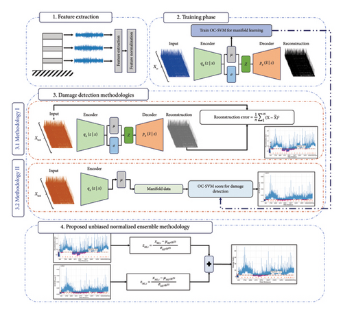
In the first stage, feature extraction from raw data is processed to extract meaningful features from vibration signals. These features are the normalized fast-Fourier transform (FFT), which is directly obtained from the time-series acceleration response of the structure. The training phase includes the VAE network that is responsible for learning manifold representations of the data. This phase uses an input dataset X_ZS from a source structure in a zero-shot learning context. The input data are passed through an encoder that generates latent variables μ and σ, encapsulating the underlying distribution of the source structure’s features. The decoder then reconstructs the input from these latent variables, allowing the VAE to learn the manifold data. In addition, an OCSVM model is trained on the manifold features of the structure to enable anomaly detection in the next phases.

The third component focuses on the damage detection procedure, which can be divided into two methodologies. The first, Methodology I, utilizes the VAE RE as the main feature. The input test data X_test from the upcoming data stream with an unknown condition are processed through the trained VAE. The RE, the difference between the original input and the reconstructed error, is calculated. This RE is then used as a metric for detecting damage with significant deviations from normal RE patterns, indicating potential damage. The second approach, Methodology II, involves utilizing the latent manifold data generated from the encoder without directly focusing on the RE. Instead, the manifold data are fed into the pretrained OCSVM model in the training phase, which computes an anomaly score. This score is used to identify damage in the target structure, with higher scores suggesting more significant deviations from the normal state.

In the final section of the flowchart, a proposed unbiased normalized ensemble methodology is outlined, which integrates the outputs of both methodologies in a statistically unbiased manner. This approach aims to provide a more reliable damage detection framework by combining the strengths of RE and manifold learning. The ensemble methodology uses normalized values of the RE and manifold data , subtracting the mean and dividing by the standard deviation for both values to contribute to the damage detection process. The normalized values are then summed to produce a final score highlighting the most likely damaged regions, providing a more robust and balanced detection method. By combining these techniques, the framework seeks to enhance the accuracy and reliability of damage detection in zero-shot SHM.

3. Dataset

In this study, two benchmark datasets with various damaged and undamaged cases were used. Datasets include (i) Qatar University Grandstand Simulator (QUGS) [62], a scaled stadium seating platform structure excited in a laboratory setting, and (ii) Yellow Frame [63], a four-story steel frame under ambient excitation. Independent research groups made the datasets publicly available. In all datasets, damaged cases are labeled as DCXX, where XX represents different damaged conditions, each identified by a unique label number.

3.1. The Yellow Frame

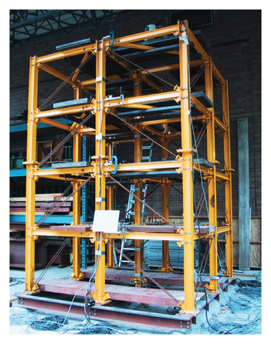
A four-story steel frame structure, built at one-third scale and incorporating modular components such as masses, braces, and columns, serves as a versatile benchmark for SHM and control studies (see Figure 4). This study focuses on the recent “brace removal” scenario involving 21 distinct data cases. Mendler et al. [63] elaborate on the sensor setup and labeling details, while a comprehensive description of the 21 data cases is provided by Bernagozzi et al. [65] and summarized in Table 1. Data acquisition was carried out at a sampling rate of 1000 Hz.

Table 1. Data cases in the Yellow Frame dataset.

Damage case	Removed brace ID
No-damage	None
DC1	2, 4 (II)
DC2	DC1 + (18, 20) (II)
DC3	DC2 + (1, 3, 17, 19) (II)
DC4	DC1 + (17, 19) (II)
DC5	DC1 + (18, 20) (I)
DC6	2 (II)
DC7	(2, 4) (I)
DC8	(25, 27) (I)
DC9	(29, 31, 8, 6) (I)
DC10	(21, 23, 29, 31) (I)
DC11	DC10 + (17, 19, 25, 27) (I)
DC12	DC7 + (1, 3, 17, 18) (I)
DC13	(10, 12) (II)
DC14	DC13 + 21 (II), 23 (I)
DC15	(21, 23) (II)
DC16	(7-8, 21, 22) (I)
DC17	(5, 6, 7, 8, 21, 24) (I)
DC18	DC17 + (7, 8, 21, 22) (I)
DC19	DC18 + (5, 6, 23, 24) (I)
DC20	(6, 8) (II), (21, 22, 23, 24) (I)

3.2. The QUGS

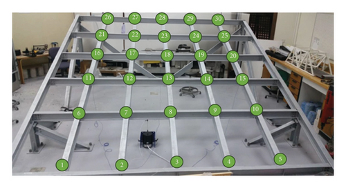
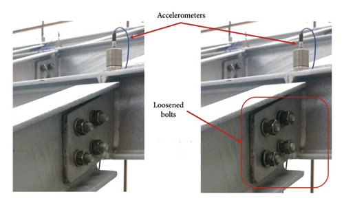
The QUGS structure is an inclined steel frame (Figure 5(a)) designed to represent a stadium spectator seating format in a structure. Avci et al. [66] elaborates on structural specifications and instrumentation of this experiment. With 30 girder connections [67, 68], QUGS damage cases are defined by bolt loosening (30 damage data cases from DC1 to DC31). Thirty accelerometers collected data at 30 joint locations with a sampling rate of 1000 Hz (Figure 5(b)).

3.3. Experimental Setup

This study analyzes the data from multiple benchmarks, where each dataset consists of time-series signals collected from various sensors. The first step involves windowing the continuous time-series data by dividing it into smaller segments of length W. Each window serves as an independent data instance for further analysis. To extract relevant features, the FFT is applied to each windowed segment channelwise, converting the data from the time domain to the frequency domain. This transformation offers a refined feature space suited to damage detection [46] without losing data dimensions.

Following the application of the FFT on data windows and the computation of the magnitude for each window, the resulting values are normalized by dividing each by its mean. This normalization is performed for all data channels across the different benchmarks. As a result, each channel’s FFT feature has dimensions of W/2, and the FFT features of all channels are concatenated synchronously into a matrix, with dimensions N × W/2, where N represents the number of channels. For example, choosing W = 1000, the QUGS dataset results in 262 data instances. There are 668 instances for the no-damage class for the Yellow Frame dataset, while the number of data instances in the damage classes ranges between 559 and 1173. Therefore, the input data size (half-spectrum FFT features) is represented as (i.e., N = 15) for the Yellow Frame dataset, while for QUGS, it is a double-struck cap R to the 15,000 (i.e., N = 30).

In this experiment, the training procedure for the neural network models is as follows. In accordance with the zero-shot setting, and to simulate online data acquisition from benchmark data, the first 50% of the no-damage class from each benchmark is treated as incoming online data. This subset is further divided into training and validation sets in a 4:1 ratio, using the feature extraction scheme described earlier. The neural networks are trained on the training set using the ADAM optimizer [69], with a recommended learning rate of 1e − 4 and decay rates of 0.9 and 0.999 for the first and second moments, respectively. The model with the lowest validation error is selected as the final model. RE is used as one metric, while the manifold representations obtained from the trained model are used to train an OCSVM on the same training and validation data. The negative of the OCSVM anomaly score (S) for each sample serves as the output for SDD. Subsequently, REs and manifold representations are computed for each sample in the remaining 50% of the no-damage data, as well as for all damage data.

For the SDD approach, four possible outcomes are expected for each incoming data point:

1.
True positive (TP), damage data, where the negative of the OCSVM score S exceeds the threshold τ.
2.
False positive (FP), no-damage data, where S exceeds τ.
3.
True negative (TN), no-damage data, where S is below τ.
4.
False negative (FN), damage data, where S is below τ.

Here, no-damage data are considered the negative class, and damage data are treated as the positive class. Based on these outcomes, the precision and recall are computed as follows:

()

The F1-score, which combines both precision and recall, is computed as follows:

()

These metrics are used to evaluate the performance of each network architecture and approach. Given the zero-shot learning nature of the proposed methodology, each dataset is divided into binary damage/no-damage classes, and accuracy measures are reported for each damage class individually. For example, in the QUGS dataset, we evaluate the 50% unobserved no-damage class data combined with each of the 30 damage cases, simulating a zero-shot damage detection scenario. For the manifold learning approach, the same 50% of no-damage data is used to obtain encoder outputs, which are then used to train an OCSVM with the extracted features.

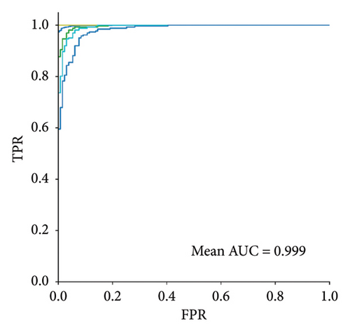
In addition, the receiver operating characteristic (ROC) curve is utilized to assess the overall performance of the models. The ROC curve plots the TP rate (TPR) against the FP rate (FPR) across different threshold values τ. The area under the ROC curve (AUC) is calculated to quantify the model’s ability to distinguish between damaged and undamaged data. A higher AUC indicates better discrimination capability, whereas a model with an AUC close to 1 suggests high accuracy in distinguishing between damage and no-damage classes.

4. Experimental Results

This section applies the proposed methodology, which uses RE and manifold data for SDD, to the two benchmark datasets, and then the performance of each approach is compared individually. The performance metrics of both approaches are presented and discussed for the potential of using RE, as well as the manifold data of the VAE networks for SDD problems. Finally, a detailed computational complexity analysis will test whether the method complies with real-world applications. Subsequently, the performance metrics of the proposed unbiased ensemble approach are presented and discussed, highlighting how the integration of both reconstruction error and manifold data from the VAE networks enhances the accuracy of SDD.

4.1. QUGS

According to Section 3.2., the QUGS dataset contains one no-damage condition and 30 different damage conditions. Half of the available no-damage data (131) is used for the training phase of the VAE network. The network is trained in a zero-shot learning manner without previous information about the structure’s condition. Figures 6(a) and 6(b) show the result of the VAE REs and the negative OCSVM anomaly score of the manifold data for damage detection, in contrast to the proposed ensemble method.

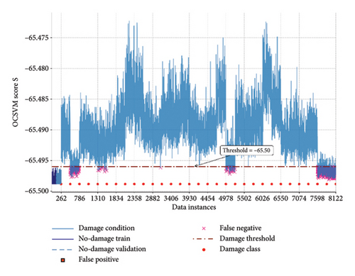
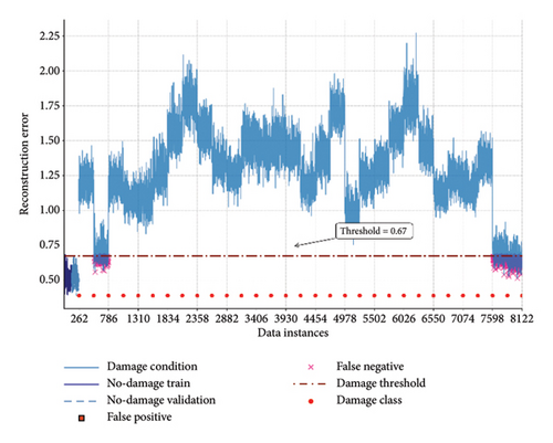
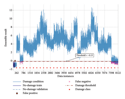
According to Figure 6 the VAE results for both the RE and manifold learning–based approaches are shown relative to the damage detection threshold. The damage detection scores indicate that both methods leverage the VAE network’s discriminative capability to identify damages, with Conditions 2, 29, and 30 proving to be more challenging for detection.

The manifold learning through OCSVM confirms that zero-shot manifold learning with VAEs can be adopted for SDD. The result of manifold learning contains more false alarms than the RE; however, it still confirms the capability of the intermediate network data to detect damage. This observation suggests that relying on the outputs of intermediate network layers may not always be the most effective approach. Therefore, proposing a reliable method to ensemble these two responses is essential for improving the performance of the VAE network in zero-shot damage detection. As shown in the results of Figure 6(c), it is evident that the proposed ensemble algorithm has significantly fewer false alarms compared to both classic decision-making damage detection techniques. It demonstrates superior power and performance relative to the proposed ensemble method for both algorithms, which leads to a lower damage index value output and makes better discrimination to identify the damage in Conditions 2, 29, and 30.

Figure 7 represents the F1-score, precision, and recall metrics obtained for better comparison according to (14)–(16). These metrics can be obtained through binary classification to assess their performance. All the above statements of the VAE network’s performance through successes and limitations of the proposed ensemble method can be figured out.

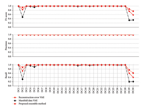
The results in Figure 7 reaffirm the observations made in Figure 6, while the RE of the VAE network demonstrates more robust performance compared to the manifold data, and the proposed ensemble method achieves the best performance. The F1-score indicates that the ensemble approach effectively outperforms the individual methods, owing to its unique and unbiased strategy. By leveraging both the RE and manifold data, the ensemble method enhances robustness through the integration of multiple perspectives, resulting in a more reliable assessment of damage detection.

In Figure 8, the class-by-class ROC curves of the QUGS structure for each approach are presented, providing a visual representation of the detection capability across different damage classes. The mean AUC of the ensemble method is higher than both the RE and the manifold data. This demonstrates that the ensemble method offers a more comprehensive and accurate detection strategy, as AUC is a key metric for assessing the performance of classification models. The higher AUC values confirm the greater sensitivity and specificity of the proposed ensemble method.

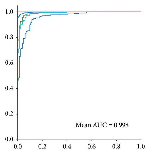
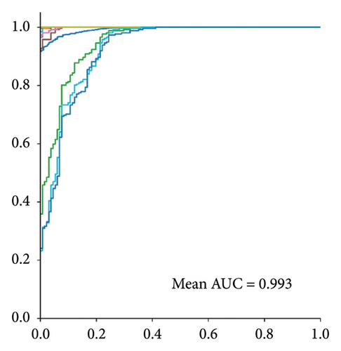
Together, these performance metrics, F1-score and AUC, underscore the effectiveness of the proposed ensemble strategy. By combining the strengths of RE and manifold data, the ensemble approach offers a balanced, reliable, and improved damage detection framework, further validating its applicability in this context.

4.2. Yellow Frame Results

This experimental evaluation of the proposed approach and VAE-based reconstruction error and manifold learning approaches on a real-scale structure under environmental and operational effects is conducted. To achieve this, the network is trained using 40% of no-damage data, or 267 data instances. This experiment is perfect for evaluating proposed approaches under imbalanced data conditions due to a variety of 559–1173 data samples for each damage case.

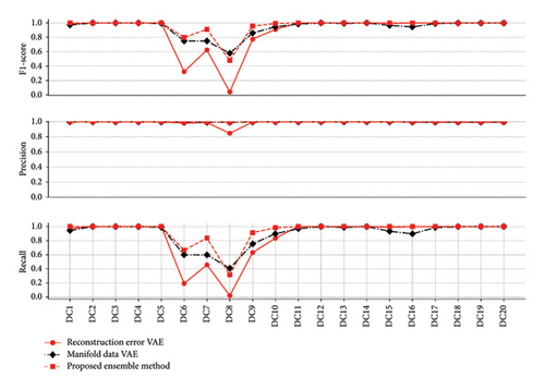
Figure 9, depicts the results of the VAE network for damage detection. In contrast to the previous result, the manifold learning approach demonstrates superior performance over the reconstruction-based method, with both showing a clear separation between most damage classes and the no-damage data. This contrasts with the results from the QUGS model, where the reconstruction approach outperformed the manifold learning. Such a discrepancy reinforces the research objective of highlighting performance variations and the necessity of developing more robust designs for real-world applications of VAE models in zero-shot SHM scenarios. This difference becomes particularly evident in the case of DC8, where the reconstruction loss fails to distinguish its instances, whereas the manifold learning approach partially captures the data, potentially indicating actual damage in practical applications.

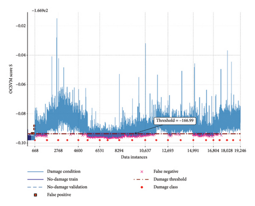
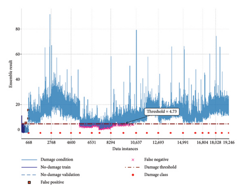
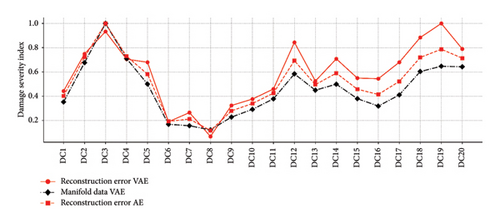
Furthermore, in this experiment, certain damage conditions involve incremental damage classes, where damages are added sequentially on top of each other. In such cases, the model can also demonstrate its capability to measure damage severity. For example, the DC2–DC5 damage conditions are derived from DC1, where the DC3 has the highest damage severity in this group regarding the number of removed braces. In addition, the damage severity of DC12 is greater than that of DC7, and DC11 is greater than that of DC10. Furthermore, the damage severity in DC17, DC18, and DC19 increased.

Figure 10 depicts the damage severity diagnosis for the Yellow Frame structure. The Euclidean distance of each data instance from the whole no-damage data was calculated to achieve this. Then, for each damage condition, the average of this distance was obtained as a final damage severity index. According to the results presented in Figure 10, all the statements about the severity of different damage conditions for this structure are fully confirmed and captured following progressive damage cases in Table 1. It should be mentioned that the damage severity results are normalized between 0 and 1.

The F1-score, precision, and recall metrics evaluation results for different approaches are presented in Figure 11, and generally, the VAE has better results for both the SDD approaches. However, the manifold data of the VAE network offer better performance at some points than the other approaches.

In addition to detection performance, the computational efficiency of the proposed framework plays a critical role in real-world SHM applications. To evaluate its practicality, we measured the execution time of key components on a mid-range NVIDIA RTX 3050 Ti GPU. As summarized in Table 2, training the VAE using 267 (40% of training data) samples with 7500 features and a batch size of 200 required approximately 2.06 min. FFT preprocessing of time-series data into the frequency domain took 0.11 min for 100 samples. The OCSVM, trained on the compact latent manifold features extracted from the VAE, completed in under one second. Notably, the entire inference pipeline, which includes FFT transformation, loading pretrained VAE weights, encoding test data, computing OCSVM scores, and ensemble calculation, was executed in under 0.225 min for a batch of 256 test samples. These results confirm the method’s suitability for periodic or near-real-time SHM, with minimal computational overhead and no reliance on labeled damage data, thus supporting efficient and scalable deployment in real-world environments.

Table 2. Runtime performance of the proposed method on RTX 3060 GPU.

Component	Time (RTX 3050 Ti)	Notes
FFT preprocessing	0.11 min	Per batch of 100 samples (time-series to frequency domain)
VAE training	2.06 min	200 batch size; 7500 features; LSTM encoder
OCSVM training	< 1 s	On low-dimensional latent (manifold) features
Inference	< 0.225 min	FFT + load pretrained VAE + OCSVM + ensemble (256 s time data samples)

4.3. Comparative Study

In the competitive study, the AE network architecture was used to evaluate the performance of various approaches, with the F1-score as the key metric across the QUGS and the Yellow Frame benchmark experiments.

As shown in Table 3, the proposed ensemble method delivered the highest performance across both datasets, achieving an F1-score of 0.983 for the QUGS and 0.955 for the Yellow Frame. While effective, the VAE-based approaches did not outperform the ensemble method. Specifically, the VAE RE achieved F1-scores of 0.972 for the QUGS and 0.880 for the Yellow Frame, while VAE manifold learning scored 0.935 for the QUGS and 0.934 for the Yellow Frame. The AE RE approach had lower performance, scoring 0.803 for the QUGS and 0.844 for the Yellow Frame. A close assessment of the outcomes can shed light on the reason behind this observation. First, by examining both QUGS (see Figure 6) and Yellow Frame (see Figure 9) results, it becomes evident that the reconstruction loss offers better discerning capacity between different damage classes, that is, their damage detection scores become more separable, while the manifold learning–based strategy is less effective in this regard. However, the improved ability to distinguish between different types of damage comes with a trade-off: an increased risk of FNs and sensitivity to threshold tuning. The more sensitive the model becomes to changes, the more likely it is for no-damage data to show sudden increases in detection scores, thereby raising the damage detection threshold and potentially leaving many real damages undetected. The proposed ensemble strategy, however, seeks to leverage the high sensitivity of the reconstruction-based approach while benefiting from the more robust damage estimation offered by the manifold-based strategy. The proposed ensemble demonstrates the significant impact of the proposed ensemble method across both datasets, confirming earlier observations that while the VAE network provides robust performance in both reconstruction and manifold data, it remains inconsistent compared to the AE network. In particular, VAE RE performed better for QUGS, while VAE manifold learning successfully detected damage conditions (DC8) in the Yellow Frame structure. Although the VAE network performs well for these benchmarks, the proposed ensemble method, by combining both strategies, enhances the overall robustness and reliability of the system. Ensemble techniques do not guarantee a superior performance compared to each of their input models, yet herein, the unbiased normalized ensemble methodology yielded superior performance in both datasets and on all, except one, damage cases, demonstrating its prowess and effectiveness in the studied zero-shot SDD benchmark problems.

Table 3. The F1-score comparison for all experiments.

Approach	Dataset
Approach	QUGS	Yellow frame
VAE reconstruction error	0.972	0.880
VAE manifold learning	0.935	0.934
AE reconstruction error	0.803	0.844
Proposed ensemble method	0.983	0.955

Note: The bold formatting in the results table is intended to highlight the performance of the proposed method.

5. Conclusions

This study proposes the unbiased normalized ensemble methodology, a robust zero-shot learning framework for structural damage detection that integrates reconstruction error and latent manifold features extracted from VAEs. In addition, this research conducted a comprehensive comparison between RE and manifold learning by employing AE and VAE models in the context of zero-shot SDD. The results revealed that the features extracted from the VAE, namely, RE and manifold representation, exhibited distinct capabilities in capturing and representing structural anomalies, even without labeled training data, outperforming traditional AE models. While the AE’s RE directly reflects the model’s ability to reproduce the structural characteristics of both undamaged and damaged data, the VAE’s probabilistic framework is shown to generate more diverse and structured reconstructions, highlighting its potential for enhanced anomaly detection in previously unseen scenarios.

The exploration into manifold learning highlighted its role in revealing the intrinsic representations of structural data within the latent space. By focusing on capturing the underlying data distribution, the VAE demonstrated a superior ability to preserve the manifold, which allowed for more meaningful interpolations between latent variables than the AE. This suggests that manifold learning offers a detailed understanding of structural variations, which is crucial for accurate damage detection in real-world applications. Moreover, by investigating both the manifold features and reconstruction loss for distinguishing damage classes in a zero-shot setting, a zero-shot damage severity measure is also proposed and demonstrated to be effective in the studied benchmarks.

Finally, the study introduced an unbiased normalized ensemble methodology that combined the outputs of both RE and manifold learning. This approach enabled more robust decision-making in zero-shot learning scenarios, where uncertainty is heightened due to the absence of labeled damaged data. By leveraging the strengths of both features, the ensemble method enhanced the reliability and accuracy of SDD.

In conclusion, this research offers valuable insights into selecting unsupervised learning models for zero-shot SDD. The observed trade-offs between RE and manifold representation underscore the importance of aligning model capabilities with the specific requirements of SHM applications. Future research could further optimize these models, incorporate domain-specific knowledge to improve detection performance, and extend the evaluation to a broader range of structural datasets, ensuring the models’ generalization and robustness across diverse SHM scenarios.

Conflicts of Interest

The authors declare no conflicts of interest.

Funding

No funding was received for this study.

Acknowledgments

The authors appreciate the Yellow Frame data provided by Dr. Carlos Ventura and Dr. Alexander Mendler.

Open Research

Data Availability Statement

The data that support the findings of this study are available from the corresponding author upon reasonable request.

References

1 Farrar C. R. and Worden K., An Introduction to Structural Health Monitoring, CISM International Centre for Mechanical Sciences. (2010) 520, 1–17, https://doi.org/10.1007/978-3-7091-0399-9_1, 2-s2.0-85017411955.
10.1007/978-3-7091-0399-9_1
Google Scholar
2 Sohn H., Farrar C. R., Hemez F. M. et al., A Review of Structural Health Monitoring Literature: 1996–2001, 2003, Los Alamos National Laboratory.
Google Scholar
3 Farrar C. R. and Worden K., Structural Health Monitoring: A Machine Learning Perspective, 2012, John Wiley & Sons.
10.1002/9781118443118
Google Scholar
4 Zhang W., Sun R., Ni P., Zhao M., El Naggar M. H., and Du X., Quantitative Analysis of Subway Station Seismic Deformation Under Random Earthquakes and Uncertain Soil Properties Using the Equivalent Linearization Method, Soil Dynamics and Earthquake Engineering. (2025) 188, https://doi.org/10.1016/j.soildyn.2024.109086.
10.1016/j.soildyn.2024.109086
Web of Science® Google Scholar
5 Reynders E., Teughels A., and De Roeck G., Finite Element Model Updating and Structural Damage Identification Using OMAX Data, Mechanical Systems and Signal Processing. (2010) 24, no. 5, 1306–1323, https://doi.org/10.1016/j.ymssp.2010.03.014, 2-s2.0-77953323926.
10.1016/j.ymssp.2010.03.014
Web of Science® Google Scholar
6 Majumdar A., Maiti D. K., and Maity D., Damage Assessment of Truss Structures from Changes in Natural Frequencies Using Ant Colony Optimization, Applied Mathematics and Computation. (2012) 218, no. 19, 9759–9772, https://doi.org/10.1016/j.amc.2012.03.031, 2-s2.0-84860485145.
10.1016/j.amc.2012.03.031
Web of Science® Google Scholar
7 Malekghaini N., Ghahari F., Ebrahimian H., Bowers M., Azari H., and Taciroglu E., Time-Domain Finite Element Model Updating for Operational Monitoring and Damage Identification of Bridges, Structural Control and Health Monitoring. (2023) 2023, 1–21, https://doi.org/10.1155/2023/4170149.
10.1155/2023/4170149
Web of Science® Google Scholar
8 Li Q., Ni P., Du X., Han Q., Xu K., and Bai Y., Bayesian Finite Element Model Updating with a Variational Autoencoder and Polynomial Chaos Expansion, Engineering Structures. (2024) 316, https://doi.org/10.1016/j.engstruct.2024.118606.
10.1016/j.engstruct.2024.118606
Web of Science® Google Scholar
9 Li Q., Ni P., Du X., Han Q., Xu K., and Bai Y., Bayesian Updating Using Accelerated Hamiltonian Monte Carlo with gradient-enhanced Kriging Model, Computers & Structures. (2025) 307, https://doi.org/10.1016/j.compstruc.2024.107598.
10.1016/j.compstruc.2024.107598
Web of Science® Google Scholar
10 Fugate M. L., Sohn H., Farrar C. R., Fugate H., Farrar C. R., and Ml S., Vibration-Based Damage Detection Using Statistical Process Control, Mechanical Systems and Signal Processing. (2001) 15, no. 4, 707–721, https://doi.org/10.1006/mssp.2000.1323, 2-s2.0-0035391479.
10.1006/mssp.2000.1323
Web of Science® Google Scholar
11 Figueiredo E., Park G., Farrar C. R. et al., Machine Learning Algorithms for Damage Detection Under Operational and Environmental Variability, Structural Health Monitoring. (2010) 10, no. 6, 559–572, https://doi.org/10.1177/1475921710388971, 2-s2.0-80455123889.
10.1177/1475921710388971
Web of Science® Google Scholar
12 Gul M. and Necati Catbas F., Statistical Pattern Recognition for Structural Health Monitoring Using Time Series Modeling: Theory and Experimental Verifications, Mechanical Systems and Signal Processing. (2009) 23, no. 7, 2192–2204, https://doi.org/10.1016/j.ymssp.2009.02.013, 2-s2.0-67349128320.
10.1016/j.ymssp.2009.02.013
Web of Science® Google Scholar
13 Figueiredo E., Damage Identification in Civil Engineering Infrastructure Under Operational and Environmental Conditions, 2010, Thesis Faculty of Engineering of the University of Porto.
Google Scholar
14 Heravi M. A., Tavakkoli S. M., and Entezami A., Structural Health Monitoring by Probability Density Function of Autoregressive-based Damage Features and Fast Distance Correlation Method, Journal of Vibration and Control. (2021) 28, no. 19-20, 2786–2802, https://doi.org/10.1177/10775463211020198.
10.1177/10775463211020198
Web of Science® Google Scholar
15 Sarmadi H., Entezami A., Behkamal B., and De Michele C., Partially Online Damage Detection Using long-term Modal Data Under Severe Environmental Effects by Unsupervised Feature Selection and Local Metric Learning, Journal of Civil Structural Health Monitoring. (2022) 12, no. 5, 1043–1066, https://doi.org/10.1007/s13349-022-00596-y.
10.1007/s13349-022-00596-y
Web of Science® Google Scholar
16 Zhang X. and Li L., An Unsupervised Learning Damage Diagnosis Method Based on Virtual Impulse Response Function and Time Series Models, Measurement. (2023) 211, https://doi.org/10.1016/j.measurement.2023.112635.
10.1016/j.measurement.2023.112635
Web of Science® Google Scholar
17 Goi Y. and Kim C. W., Bridge Damage Detection Using Ambient Loads by Bayesian Hypothesis Testing for a Parametric Subspace of an Autoregressive Model, Structural Control and Health Monitoring. (2023) 2023, no. 1, 7986061–20, https://doi.org/10.1155/2023/7986061.
10.1155/2023/7986061
Web of Science® Google Scholar
18 Fakharian P. and Naderpour H., Damage Severity Quantification Using Wavelet Packet Transform and Peak Picking Method, Practice Periodical on Structural Design and Construction. (2022) 27, no. 1, 1–11, https://doi.org/10.1061/(asce)sc.1943-5576.0000639.
10.1061/(asce)sc.1943-5576.0000639
Web of Science® Google Scholar
19 Li H., Deng X., Dai H., Li X., and Dai H. H. D., Structural Damage Detection Using the Combination Method of EMD and Wavelet Analysis, Mechanical Systems and Signal Processing. (2007) 21, no. 1, 298–306, https://doi.org/10.1016/j.ymssp.2006.05.001, 2-s2.0-33749535038.
10.1016/j.ymssp.2006.05.001
Web of Science® Google Scholar
20 Shi Z. Y., Law S. S., and Xu X., Identification of Linear time-varying Mdof Dynamic Systems from Forced Excitation Using Hilbert Transform and EMD Method, Journal of Sound and Vibration. (2009) 321, no. 3–5, 572–589, https://doi.org/10.1016/j.jsv.2008.10.005, 2-s2.0-60349101382.
10.1016/j.jsv.2008.10.005
Web of Science® Google Scholar
21 Xu Y. L. and Chen J., Structural Damage Detection Using Empirical Mode Decomposition: Experimental Investigation, Journal of Engineering Mechanics. (2004) 130, no. 11, 1279–1288, https://doi.org/10.1061/(asce)0733-9399(2004)130:11(1279), 2-s2.0-10244226731.
10.1061/(ASCE)0733-9399(2004)130:11(1279)
Web of Science® Google Scholar
22 Silik A., Noori M., Ghiasi R. et al., Dynamic Wavelet Neural Network Model for Damage Features Extraction and Patterns Recognition, Journal of Civil Structural Health Monitoring. (2023) 13, no. 4-5, 925–945, https://doi.org/10.1007/s13349-023-00683-8.
10.1007/s13349-023-00683-8
Web of Science® Google Scholar
23 Entezami A., Sarmadi H., Behkamal B., and Mariani S., Big Data Analytics and Structural Health Monitoring: a Statistical Pattern Recognition-based Approach, Sensors. (2020) 20, no. 8, https://doi.org/10.3390/s20082328.
10.3390/s20082328
Web of Science® Google Scholar
24 Chegeni M. H., Sharbatdar M. K., Mahjoub R., and Raftari M., New Supervised Learning Classifiers for Structural Damage Diagnosis Using Time Series Features from a New Feature Extraction Technique, Earthquake Engineering and Engineering Vibration. (2022) 21, no. 1, 169–191, https://doi.org/10.1007/s11803-022-2079-2.
10.1007/s11803-022-2079-2
Web of Science® Google Scholar
25 Feizi Y. A., Sharbatdar M. K., Mahjoub R., and Raftari M., A Hybrid Unsupervised Learning Method for Structural Health Monitoring by Artificial Neural Networks and k-means Clustering, Scientia Iranica. (2023) 0, no. 0, https://doi.org/10.24200/sci.2023.61100.7141.
10.24200/sci.2023.61100.7141
Google Scholar
26 Xu C., Lei H., and Wang G., Damage Identification Method of long-span Spatial Structure Based on time-series Model of Measured Data, Journal of Civil Structural Health Monitoring. (2023) 13, no. 2-3, 693–707, https://doi.org/10.1007/s13349-023-00672-x.
10.1007/s13349-023-00672-x
Web of Science® Google Scholar
27 Hakim S. J. S. and Razak H. A., Modal Parameters Based Structural Damage Detection Using Artificial Neural Networks-A Review, Smart Structures and Systems. (2014) 14, no. 2, 159–189, https://doi.org/10.12989/sss.2014.14.2.159, 2-s2.0-84905969947.
10.12989/sss.2014.14.2.159
Web of Science® Google Scholar
28 Ghiasi R., Torkzadeh P., and Noori M., A machine-learning Approach for Structural Damage Detection Using Least Square Support Vector Machine Based on a New Combinational Kernel Function, Structural Health Monitoring. (2016) 15, no. 3, 302–316, https://doi.org/10.1177/1475921716639587, 2-s2.0-84968764363.
10.1177/1475921716639587
Web of Science® Google Scholar
29 Le-Xuan T., Bui-Tien T., and Tran-Ngoc H., A Novel Approach Model Design for Signal Data Using 1DCNN Combing with LSTM and Resnet for Damaged Detection Problem, Structures. (2024) 59, https://doi.org/10.1016/j.istruc.2023.105784.
10.1016/j.istruc.2023.105784
Web of Science® Google Scholar
30 Zhang X. and Zhou W., Structural Vibration Data Anomaly Detection Based on Multiple Feature Information Using CNN-LSTM Model, Structural Control and Health Monitoring. (2023) 2023, no. 1, 1–19, https://doi.org/10.1155/2023/3906180.
10.1155/2023/3906180
CAS Web of Science® Google Scholar
31 Figueiredo E. and Santos A., Machine Learning Algorithms for Damage Detection, Computational and Experimental Methods Series. (2018) 10, 1–39, https://doi.org/10.1142/9781786344977_0001, 2-s2.0-85051565936.
10.1142/9781786344977_0001
Google Scholar
32 Sarmadi H., Entezami A., Saeedi Razavi B., and Yuen K. V., Ensemble Learning-based Structural Health Monitoring by Mahalanobis Distance Metrics, Structural Control and Health Monitoring. (2021) 28, no. 2, 1–24, https://doi.org/10.1002/stc.2663.
10.1002/stc.2663
Web of Science® Google Scholar
33 Soleimani-Babakamali M. H., Soleimani-Babakamali R., and Sarlo R., A General Framework for Supervised Structural Health Monitoring and Sensor Output Validation Mitigating Data Imbalance with Generative Adversarial networks-generated high-dimensional Features, Structural Health Monitoring. (2022) 21, no. 3, 1167–1182, https://doi.org/10.1177/14759217211025488.
10.1177/14759217211025488
Web of Science® Google Scholar
34 Goodfellow I. B. Y. C. A., Greedy Layer-wise Unsupervised Pretraining, Deep Learning. (2016) 10, 526–527.
Google Scholar
35 Figueiredo E., Figueiras J., Park G., Farrar C. R., and Worden K., Influence of the Autoregressive Model Order on Damage Detection, Computer-Aided Civil and Infrastructure Engineering. (2011) 26, no. 3, 225–238, https://doi.org/10.1111/j.1467-8667.2010.00685.x, 2-s2.0-79951564510.
10.1111/j.1467-8667.2010.00685.x
Web of Science® Google Scholar
36 Lei X., Sun M., Zhao R. et al., Unsupervised Vision-based Structural Anomaly Detection and Localization with Reverse Knowledge Distillation, Structural Control and Health Monitoring. (2024) 2024, no. 1, https://doi.org/10.1155/2024/8933148.
10.1155/2024/8933148
Web of Science® Google Scholar
37 Goodfellow I., Bengio Y., and Courville A., Deep Learning, 2016.
Google Scholar
38 Eltouny K., Gomaa M., and Liang X., Unsupervised Learning Methods for Data-Driven Vibration-based Structural Health Monitoring: a Review, Sensors. (2023) 23, no. 6, https://doi.org/10.3390/s23063290.
10.3390/s23063290
Web of Science® Google Scholar
39 Silva M. F., Santos A., Santos R., Figueiredo E., and Costa J. C. W. A., Damage-Sensitive Feature Extraction with Stacked Autoencoders for Unsupervised Damage Detection, Structural Control and Health Monitoring. (2021) 28, no. 5, 1–19, https://doi.org/10.1002/stc.2714.
10.1002/stc.2714
CAS Web of Science® Google Scholar
40 Eltouny K. and Liang X., A Nonparametric Unsupervised Learning Approach for Structural Damage Detection, ArXiv. (2020) 2009.
Google Scholar
41 Wang Z. and Cha Y., Unsupervised Machine and Deep Learning Methods for Structural Damage Detection: a Comparative Study, Engineering Reports. (2022) 7, 1–23, https://doi.org/10.1002/eng2.12551.
10.1002/eng2.12551
Web of Science® Google Scholar
42 Wang Z., A Novel Unsupervised Deep Learning Method with a Convolutional Neural Network for Structural Damage Detection, Conference Proceedings of the Society for Experimental Mechanics Series, August 2023, Milwaukee, WI, 105–112, https://doi.org/10.1007/978-3-031-05445-7_12.
10.1007/978-3-031-05445-7_12
Google Scholar
43 Zhang Y., Xie X., Li H., and Zhou B., An Unsupervised Tunnel Damage Identification Method Based on Convolutional Variational Auto-Encoder and Wavelet Packet Analysis, Sensors. (2022) 22, no. 6, https://doi.org/10.3390/s22062412.
10.3390/s22062412
Web of Science® Google Scholar
44 Soleimani-Babakamali M. H., Sepasdar R., Nasrollahzadeh K., Lourentzou I., and Sarlo R., Toward a General Unsupervised Novelty Detection Framework in Structural Health Monitoring, Computer-Aided Civil and Infrastructure Engineering. (2022) 37, no. 9, 1128–1145, https://doi.org/10.1111/mice.12812.
10.1111/mice.12812
Web of Science® Google Scholar
45 Soleimani-Babakamali M. H., Soleimani-Babakamali R., Sarlo R., Farghally M. F., and Lourentzou I., On the Effectiveness of Dimensionality Reduction for Unsupervised Structural Health Monitoring Anomaly Detection, Mechanical Systems and Signal Processing. (2023) 187, https://doi.org/10.1016/j.ymssp.2022.109910.
10.1016/j.ymssp.2022.109910
Web of Science® Google Scholar
46 Soleimani-Babakamali M. H., Sepasdar R., Nasrollahzadeh K., and Sarlo R., A System Reliability Approach to real-time Unsupervised Structural Health Monitoring Without Prior Information, Mechanical Systems and Signal Processing. (2022) 171, https://doi.org/10.1016/j.ymssp.2022.108913.
10.1016/j.ymssp.2022.108913
Web of Science® Google Scholar
47 Entezami A., De Michele C., Arslan A. N., and Behkamal B., Detection of Partially Structural Collapse Using Long-Term Small Displacement Data from Satellite Images, Sensors. (2022) 22, no. 13, https://doi.org/10.3390/s22134964.
10.3390/s22134964
Web of Science® Google Scholar
48 Lei X., Sun L., and Xia Y., Lost Data Reconstruction for Structural Health Monitoring Using Deep Convolutional Generative Adversarial Networks, Structural Health Monitoring. (2021) 20, no. 4, 2069–2087, https://doi.org/10.1177/1475921720959226.
10.1177/1475921720959226
Web of Science® Google Scholar
49 Soleimani-Babakamali M. H., Soleimani-Babakamali R., Nasrollahzadeh K., Avci O., Kiranyaz S., and Taciroglu E., Zero-Shot Transfer Learning for Structural Health Monitoring Using Generative Adversarial Networks and Spectral Mapping, Mechanical Systems and Signal Processing. (2023) 198, https://doi.org/10.1016/j.ymssp.2023.110404.
10.1016/j.ymssp.2023.110404
Web of Science® Google Scholar
50 Chen M., Mangalathu S., and Jeon J. S., Rapid Damage State Identification of Structures Using Generalized zero-shot Learning Method, Earthquake Engineering & Structural Dynamics. (2024) 9, https://doi.org/10.1002/eqe.4218.
10.1002/eqe.4218
Google Scholar
51 Kiranyaz S., Devecioglu O. C., Alhams A. et al., Zero-Shot Motor Health Monitoring by Blind Domain Transition, Mechanical Systems and Signal Processing. (2024) 210, https://doi.org/10.1016/j.ymssp.2024.111147.
10.1016/j.ymssp.2024.111147
Web of Science® Google Scholar
52 Neloy A. A. and Turgeon M., A Comprehensive Study of auto-encoders for Anomaly Detection: Efficiency and trade-offs, Machine Learning with Applications. (2024) 17, https://doi.org/10.1016/j.mlwa.2024.100572.
10.1016/j.mlwa.2024.100572
Web of Science® Google Scholar
53 Kingma D. and Welling M., Auto-Encoding Variational Bayes, 2014.
Google Scholar
54 Wang W., Huang Y., Wang Y., and Wang L., Generalized Autoencoder: A Neural Network Framework for Dimensionality Reduction, 2014 IEEE Conference on Computer Vision and Pattern Recognition Workshops, June 2014, Columbus, OH, 496–503, https://doi.org/10.1109/CVPRW.2014.79, 2-s2.0-84908500543.
10.1109/CVPRW.2014.79
Google Scholar
55 Hearst M. A., Dumais S. T., Osuna E., Platt J., and Scholkopf B., Support Vector Machines, IEEE Intelligent Systems and Their Applications. (1998) 13, no. 4, 18–28, https://doi.org/10.1109/5254.708428, 2-s2.0-11644275559.
10.1109/5254.708428
Web of Science® Google Scholar
56 Behkamal B., Entezami A., De Michele C., and Arslan A. N., Elimination of Thermal Effects from Limited Structural Displacements Based on Remote Sensing by Machine Learning Techniques, Remote Sensing. (2023) 15, no. 12, https://doi.org/10.3390/rs15123095.
10.3390/rs15123095
Web of Science® Google Scholar
57 Jiang K., Han Q., Du X., and Ni P., A Decentralized Unsupervised Structural Condition Diagnosis Approach Using Deep auto-encoders, Computer-Aided Civil and Infrastructure Engineering. (2021) 36, no. 6, 711–732, https://doi.org/10.1111/mice.12641.
10.1111/mice.12641
Web of Science® Google Scholar
58 Rosafalco L., Manzoni A., Mariani S., and Corigliano A., An Autoencoder-based Deep Learning Approach for Load Identification in Structural Dynamics, Sensors. (2021) 21, no. 12, 4207–4232, https://doi.org/10.3390/s21124207.
10.3390/s21124207
Web of Science® Google Scholar
59 Pollastro A., Testa G., Bilotta A., and Prevete R., Semi-Supervised Detection of Structural Damage Using Variational Autoencoder and a One-Class Support Vector Machine, IEEE Access. (2023) 11, 67098–67112, https://doi.org/10.1109/ACCESS.2023.3291674.
10.1109/ACCESS.2023.3291674
Web of Science® Google Scholar
60 Ghiasi R., Khan M. A., Sorrentino D., Diaine C., and Malekjafarian A., An Unsupervised Anomaly Detection Framework for Onboard Monitoring of Railway Track Geometrical Defects Using one-class Support Vector Machine, Engineering Applications of Artificial Intelligence. (2024) 133, https://doi.org/10.1016/j.engappai.2024.108167.
10.1016/j.engappai.2024.108167
Web of Science® Google Scholar
61 Sabokrou M., Fathy M., Zhao G., and Adeli E., Deep end-to-end one-class Classifier, IEEE Transactions on Neural Networks and Learning Systems. (2021) 32, no. 2, 675–684, https://doi.org/10.1109/TNNLS.2020.2979049.
10.1109/TNNLS.2020.2979049
PubMed Web of Science® Google Scholar
62 Avci O., Abdeljaber O., Kiranyaz M. S., Boashash B., Sodano H., and Inman D. J., Efficiency Validation of One Dimensional Convolutional Neural Networks for Structural Damage Detection Using A SHM Benchmark Data, Naturalists. (2018) 8, 4600–4607.
Google Scholar
63 Mendler A., Ventura C., and Allahdadian S., The Yellow Frame: Experimental Studies and Remote Monitoring of the Structural Health Monitoring Benchmark Structure, Conference Proceedings of the Society for Experimental Mechanics Series. (2019) 5, 233–244, https://doi.org/10.1007/978-3-319-75390-4_21.
10.1007/978-3-319-75390-4_21
Google Scholar
64 Agrawal S. D. A. K., NEES: Database for Structural Control and Monitoring Benchmark Problems, 2015.
Google Scholar
65 Bernagozzi G., Ventura C., Allahdadian S., Kaya Y., Landi L., and Diotallevi P., Application of Modal Flexibilitybased Deflections for Damage Diagnosis of a Steel Frame Structure, Procedia Engineering. (2017) 199, 2026–2033, https://doi.org/10.1016/j.proeng.2017.09.468, 2-s2.0-85029903411.
10.1016/j.proeng.2017.09.468
Google Scholar
66 Avci O., Abdeljaber O., Kiranyaz S., Hussein M., and Inman D. J., Wireless and real-time Structural Damage Detection: a Novel Decentralized Method for Wireless Sensor Networks, Journal of Sound and Vibration. (2018) 424, 158–172, https://doi.org/10.1016/j.jsv.2018.03.008, 2-s2.0-85044102066.
10.1016/j.jsv.2018.03.008
Web of Science® Google Scholar
67 Abdeljaber O., Younis A., Avci O. et al., Dynamic Testing of a Laboratory Stadium Structure, Geotechnical and Structural Engineering Congress 2016. (2016) 18, 1719–1728, https://doi.org/10.1061/9780784479742.147.
10.1061/9780784479742.147
Google Scholar
68 Avci O., Abdeljaber O., Kiranyaz S., Hussein M., Gabbouj M., and Inman D., A New Benchmark Problem for Structural Damage Detection: Bolt Loosening Tests on a Large-Scale Laboratory Structure, Dynamics of Civil Structures, 2022, Springer International Publishing, https://doi.org/10.1007/978-3-030-77143-0_2.
10.1007/978-3-030-77143-0_2
Google Scholar
69 Kingma D. P. and Ba J., Adam: a Method for Stochastic Optimization.
Google Scholar

All articles

Unbiased Normalized Ensemble Methodology for Zero-Shot Structural Damage Detection Using Manifold Learning and Reconstruction Error From Variational Autoencoder

Abstract

1. Introduction