

An Attention-Based Detection Method of Fatigue Cracks on Steel
Abstract
Steel structures are susceptible to fatigue cracking under cyclic loading, which can lead to catastrophic structural failure. In the incipient phase of crack propagation, the width of fatigue cracks typically measures less than 0.1 mm, making them difficult to detect using standard imaging techniques. This study presents a novel approach to crack detection on steel structures by tracking the displacement field on the structural surface derived from visual data. Initially, video or sequential images of the target structure under loading are captured and processed using an enhanced dense feature-matching model. The surface displacement field is then computed from the coordinate difference of the numerous matched feature points. By extracting discontinuities within the displacement field, fatigue cracks can be localized. Two case studies were conducted to validate the methodology: one involving a with a pre-existing crack and another steel plate with fatigue crack propagation. The findings indicate that the proposed method can be used to detect minuscule cracks, with crack widths as small as 5 μm. Factors potentially influcencing the method, including the texture of the steel surface, the region of interest (ROI) area ratio, the density of matching, and the resolution of input images, were discussed. Compared to traditional image-based semantic segmentation techniques, this approach is more convenient and precise, offering a promising avenue for the nondestructive evaluation of steel structures in civil engineering.
1. Introduction
Steel structures are widely used in the construction of large-span buildings and bridges attributed to their superior mechanical performance, lightweight design, and ease of assembly. The steel construction industry in China experienced a notable year-on-year growth of 10.5% in 2022 [1]. Despite the widespread use, steel structures are susceptible to fatigue damage when exposed to dynamic loading. The rapid propagation of fatigue cracks can lead to severe consequences, particularly if they extend through critical structural components. However, nowadays, the detection of initial fatigue cracks remains challenging due to the small crack size.
Traditional damage detection methods, such as human inspection, are direct but inefficient, labor-intensive, and prone to subjective errors, leading to false positives and missed detections. In response to the growing emphasis on the long-term integrity of structures, structural health monitoring (SHM) systems are increasingly integrated into engineering practice. These systems utilize sensors to capture macroscopic responses of structures, which are then analyzed through modal analysis to assess potential damage. For instance, optical fiber sensors are employed to measure various parameters such as frequency, acceleration, and strain. By leveraging these data for modal and reliability analyses, engineers can identify damage and predict the remaining life of structures. However, implementing a comprehensive SHM system is often expensive, complex, and requires specialized postprocessing algorithms. Critically, the macroscopic signals captured by these systems may not be sensitive enough to effectively detect early-stage structural damage. In addition to SHM systems, various nondestructive detection techniques, including ultrasonic [2–4], thermal infrared [5], magnetic flux leakage, and LIDAR detection methods [6], offer more direct measurements of local damages. These techniques require expensive equipment and may be limited by environmental conditions. For example, the thermal infrared technique often requires a heat source, while the magnetic flux leakage technique is only suitable for ferromagnetic materials. These limitations hinder their widespread adoption. The advancement of charge-coupled device (CCD) cameras has revolutionized image acquisition by enabling rapid data capture. Coupled with the evolution of computer image processing techniques, computer vision has shown great promise in industrial inspection. Initially, methods such as image binarization and edge enhancement were employed for surface crack detection in creep–fatigue tests [7] and billets [8]. However, these techniques often produced significant noise, leading to false detections that necessitated manual interpretation. To enhance accuracy and reduce false results, postprocessing methods such as image dilation and simple filtering have been proposed. However, the efficacy of these methods is heavily influenced by input parameters, which must be adapted to specific characteristics of different images. In comparison with other surface cracks, fatigue cracks have much smaller crack widths, making them difficult to detect with standard image processing techniques. Therefore, additional image processing steps are essential for the successful detection of fatigue cracks. Common strategies involve enhancing image details using high-pass filters such as edge extraction algorithms such as Sobel [9] and Canny [10]. Sobel is a gradient operator, calculating the weighted average of the gray levels of adjacent pixels. The extreme points, considered as the sharper place of the gray scale change in the image, are selected as the cracks. Despite these efforts and advances, the performance of these algorithms is still significantly impacted by factors such as image quality, lighting conditions, resolution, and shooting angles, making their effectiveness context-specific. In pursuit of robust and accurate crack detection, there has been a notable shift toward algorithms based on machine learning techniques [11–13]. Tian et al. [14] combined genetic algorithms with extreme learning machines for defect detection on steel surfaces. The mutation ability of the genetic algorithm partly neutralized the instability of the extreme learning machine caused by random initialization. Alberto et al. [15] leveraged artificial neural networks (ANNs) for feature extraction in images of ships with corrosion and cracks using color and texture descriptors, where feature maps were input into an ANN trained with labeled images of defects. Conventional machine learning algorithms rely on manually designed feature descriptors and may struggle with complex backgrounds in cases where there are numerous scratches, handwritten texts, corrosion, and other interference factors on steel. In contrast, deep learning algorithms designed for object detection and semantic segmentation have demonstrated superior performance in distinguishing cracks from intricate backgrounds. In the direction of deep learning algorithms, Han et al. [16] introduced a comprehensive approach that incorporated SLIC superpixel segmentation for image compression, the YOLOv3 model for crack region framing, and a collaborative decision-making process involving multiple DeepLabv3+ models for pixel-level segmentation. Similarly, Zhou et al. [17] employed a faster R-CNN to pinpoint crack locations. Subsequently, a sequence of image processing techniques, including decolorization, filtering, denoising, contrast enhancement, maximum entropy threshold segmentation, and Canny edge detection, were applied to subimages within the designated region to extract crucial crack dimensions such as length, width, and area. The identification of false positives was managed through criteria based on aspect ratios and area measurement. Deng et al. [18] developed the innovative APA-Net, a hollow pyramid attention network model distinguished by its departure from conventional encoder–decoder architectures. APA-Net integrated a pretrained ResNet34 model, a dense cavity convolution module (DAC), a scale-aware pyramid fusion module (SAPF), and an attention-gating mechanism (AG) to enhance the model’s capacity for extracting multiscale contextual information. A specialized fatigue crack segmentation dataset using steel box girder images, accounting for various complicating factors to optimize model training, was collected. Another typical image segmentation neural network widely used in crack detection was U-Net [13, 19], which can assess the geometrical shape of cracks at pixel level. The U-Net structure consists of a contractive (downsampling) path and an expansive (upsampling) path. The contractive path captures the feature map of the input image, while the expansive path enables precise localization using transposed convolutions. To use the crack depth information, crack descriptor CIG [20] is calculated by estimating the crack depth, which can detect cracks by iteratively searching the salient string of pixels. These methodologies exhibited robust segmentation capabilities, particularly suited for identifying large-scale cracks that are clearly discernible within image datasets.
However, in the initial stages of fatigue crack formation and propagation, the width of cracks typically falls within the micrometer range, posing a challenge for clear visualization on a single static image. Considering the dynamic nature of fatigue cracks, which open and close under varying loads, the detection of small-scale cracks can be achieved by monitoring surface movements and recognizing abnormal areas in the displacement field [21]. This process involves two crucial steps, i.e., feature point detection and matching. Feature point detection entails identifying computer-recognizable pixel points, known as feature points, that exhibit significant pixel value changes within an image, such as corners, edges, or distinctive spots. To ensure accurate matching, feature points must possess the following characteristics: (1) uniquely identifiable within the target image, ensuring distinguishability among all detected feature points; (2) quantitatively describable by feature descriptors, providing additional information alongside the feature point itself; and (3) robust against image transformations such as panning, rotation, scaling, illumination variations, and noise, enabling the detection even with notable image alterations. Classical algorithms for feature point detection include Harris corner point [22], Shi-Tomasi corner point [23], scale-invariant feature transform (SIFT) [24], speeded up robust features (SURF) [25], FAST, oriented FAST and rotated BRIEF (ORB) [26], and SuperPoint [27]. Feature point matching involves correlating feature points between two images based on the similarity of their descriptors. Each pair of similar feature points forms a matching point pair, enabling tracking of the feature point motion across sequential images. Common feature point matching or tracking algorithms include brute-force matching, cross-matching, KNN matching, RANSAC, and sparse optical flow tracking (KLT) [28].
These algorithms facilitate the efficient identification of sparse matched points. In the realm of computer vision, feature point detection and matching find extensive utility in applications such as target tracking, image stitching, and 3D reconstruction, for which sparse matched points are sufficient. Nonetheless, the quantity of these sparse points is inadequate for comprehensive inference of a displacement field across a deformed area in the field of civil engineering. Furthermore, within regions of an image characterized by repetitive or sparse textures, the detection of feature points by these algorithms is significantly challenging. One possible solution involves determining the relative pose between two images using sparse matching points. By calculating the coordinates of the corresponding pixel in one image with respect to the other, dense matching point pairs can be generated. This method has been widely used in aerial triangulation in photogrammetry [29]. The ground coordinates of unknown points are calculated based on the elements of exterior orientation, which are inferred from a few control points. Nevertheless, this method assumes that changes in images solely result from alterations in the camera or object positions, which may not hold true since the structure deforms under loading. Another strategy involves artificially enhancing the texture and features of the surface by applying speckle patterns to the surface, which serves to increase the number of matching point pairs and enhance matching accuracy. A prominent application lies in the digital image correlation (DIC) technology, which can be used to detect cracks at submillimeter or even micrometer scales. This technique involves spraying the region of interest (ROI) with speckles to create distinctive visual feature points, whose motion is tracked to infer the overall displacement field. Crack tips are consequently determined by analyzing the convergence of displacement values [30].
However, implementation of speckling is generally complex, and quality of speckles significantly affects accuracy of the detected displacement fields. To address this challenge, multiframe images or video streams provide an opportunity since they contain more information compared to a single image, thereby having the potential of providing more matching points. Notably, Kong et al. [31] proposed a crack detection method based on video feature tracking with no artificial feature points involved. The methodology was comprised of four stages, i.e., feature point detection using the Shi-Tomasi algorithm, feature point tracking with the KLT optical flow algorithm, crack detection and localization, and quantification of crack opening. By analyzing motion patterns of the feature points, the presence of cracks on the surface was identified. This approach offered simplicity in implementation, eliminating the need for costly equipment, light sources, or specialized surface treatments. It should be pointed out that, its efficacy heavily relied on the number of feature points on the structural surface detected by the Shi-Tomasi algorithm. However, this method struggles to detect small cracks in scenarios with sparse texture where surface imperfections, such as scratches, spots, or corrosion, are absent, which leads to reduced number of feature points and indistinguishable feature descriptor.
To address the above challenges, this paper presents a novel fatigue crack detection method for steel surfaces utilizing sequential images. The approach involved closely monitoring motion of feature points within the image to infer the structural surface displacement field in the ROI and identifying fatigue cracks based on discontinuities in this field. Mutiframe dynamic images of the target structure under loading were input into a feature-matching model called detector-free local feature matching with transformers (LoFTR) [32] so that the motion of matched points could be tracked. To densely match feature points on a pair of images without distinct visual features, several improvements have been supplemented to the original LoFTR model, including the model structure, tiled subimages with overlapping regions, and displacement smoothness constraint. Since the displacement field was used to detect cracks, the proposed method was less susceptible to interference from complex backgrounds and was capable of detecting minuscule cracks that might be invisible by the naked eye or standard imaging techniques. Furthermore, in comparison with techniques combining dynamic images with DIC, this method eliminated the need for manual speckling, making it more convenient for on-site monitoring on a large scale.
2. Methodology
2.1. Overview
This section outlines the proposed methodology for crack detection in steel structures using multiframe dynamic images, as shown in Figure 1. The approach enabled the inference of the displacement field of a target component under dynamic loading, utilizing a consumer-grade digital camera without additional preprocessing of the component or its surroundings. Furthermore, the method allowed for the detection of 5-μm-width fatigue cracks by analyzing discontinuities in the displacement field surrounding the cracks. The method operated based on two primary assumptions: (1) the target region could be treated as approximately planar and (2) the camera platform was stable, meaning all the motion on the image was caused by the motion of the detected object.

Figure 1 illustrates the essential steps of crack detection: (1) dense feature point matching: dense feature points within the ROI were matched between the images at time tn and the reference image at time t0; (2) displacement field inference: displacement field was inferred from the displacements of these feature points between two time steps; (3) crack detection: potential fatigue cracks were detected based on the abrupt changes in the displacement field; and (4) crack parameter calculation: an image processing algorithm was then employed to quantify cracks.
2.2. Dense Matching of Feature Points
The detection accuracy of the displacement field and subsequently fatigue cracks are directly impacted by the matching of feature points. This section elaborates on specific procedures of feature point matching.
Commonly utilized feature point detection and matching techniques, such as SIFT, SURF, and ORB, can only detect feature points sparsely, given a limited number of matched point pairs. In a preliminary test conducted by the authors on a typical image pair of steel plates with a resolution of 3840 × 2160 (equivalent to around 8 million total pixels), the number of matching points obtained through SIFT with brute-force matching was approximately 80,000, which accounted for about 0.9% of the total pixels, including false matches. In images with sparse textures, effectively matching feature points becomes even more challenging.
To generate a continuous displacement field, it is essential to have a sufficient number and density of matching point pairs. Given the limited texture on steel surfaces, it is challenging to achieve dense feature point detection and matching. A potential solution involves computing correlations among all pixels in two images and selecting pairs with high correlation as matching point pairs. This concept forms the basis of LoFTR neural network model, which can be used to achieve dense feature matching in regions with sparse textures but at the expense of increased computational complexity. The original LoFTR model comprises four key components, i.e., a feature map extraction module utilizing a convolutional neural network (CNN), a transformer coding module based on linear attention, a coarse matching module, and a fine matching optimization module. The feature map extraction module employs convolution (downsampling) and inverse convolution (upsampling) as its backbone. It extracts feature maps of 1/8 size (, ) and 1/2 size (, ) from the input reference image (tA) and the image at the current moment (tB) (see Appendix A for details (Table A1)).
Within the transformer coding module, all generated feature maps undergo positional encoding using a 2D sine–cosine function, followed by eight attention layers comprising four self-attention layers and four cross-attention layers. Outputs of this module are denoted as , , , and , which are described in detail in Appendix A (Table A1). The coarse matching model calculates correlations among all points in and , extracting matched point pairs in integer pixel coordinates through nonmaximal suppression and thresholding. Subsequently, the fine matching model selects a window centered on each matching point in and to optimize the coordinates of each matching point pair. This process results in the determination of matching point pairs in subpixel coordinates.
Note that the original LoFTR is not sufficient for detecting the displacement field. To illustrate this, a trial test was conducted on a steel image pair (Figure 2). The original pretrained model detected 166 matched point pairs, whereas the fine-tuned model trained on the steel image detected 1840 pairs. Both quantities were far from enough to deduce the displacement field.


- 1.
Inverse convolution with higher resolution
-
To address the need for a higher density of matched point pairs, the scale of and , which set the upper limit for the number of matching point pairs generated in the coarse matching module, was increased. For instance, if each point on could potentially match a point on , when the resolution of and was 8 in width and 8 in height, the maximum number of matched point pairs could reach 64 (8 × 8). This limit could increase to 256 with a resolution of 16 × 16 (16 in width and 16 in height). To further enhance the potential number of matching point pairs, an inverse convolution layer was introduced to the feature map extraction module. This modification allowed the extraction of a feature map at a 1/1 size, matching the dimensions of the input image, and consequently facilitating the generation of more matching point pairs. The model structure is illustrated in Figure 3.
- 2.
Tiled subimages with overlapping regions
-
The original model accepted a fixed resolution (320 × 240) for the input image. When the resolution exceeded 320 × 240, the input image would be downsampled to fit this fixed size, which compromised the information in a high-resolution image. To overcome this constraint and enhance the density of matching point pairs, the input image was divided into multiple patches, each with a resolution of 320 × 240. Consequently, each pair of patches could be separately input into the model for feature matching, leading to a greater number of matching point pairs. Considering the potential deformation of the target object, a pixel near the patch boundary might move to surrounding patches. To address this issue, an overlap region was set when dividing the input image into patches. The overlap region consisted of 25% of the length of each patch and extended on four edges (Figure 4). For a pixel in patch boundary, the searching region consisted of both the patches connecting the boundary, thus improving the overall matching accuracy and robustness of the model.
- 3.
Displacement smoothness constraint
-
Given two matching point pairs, and (, the displacements dp and dq of these pairs were calculated. The dimensions and explanations of are provided in Appendix A (Table A1). As the deformation of the target was assumed to be small, the displacement field was expected to be continuous across most parts of the specimen. Even at the fatigue crack boundaries, the displacement discontinuity was expected to be small. This implied that displacements of neighboring matching pairs should be similar. Specifically, if the absolute difference between dp and dq was less than a predefined threshold ε, the two matching point pairs were considered valid. Conversely, if the displacement difference exceeded this threshold (|dp − dq| > ε), which was set as 0.5 pixel in this study, the pairs were deemed false matches and rejected. On average, over 3% of the matching pairs were false and eliminated in this step. This approach helped to improve the accuracy of the matching process by ensuring consistency in displacement values.


2.3. Displacement Field Inference Based on Discrete Matching Point Pairs
Matching point pairs ), ), …, were obtained from the image feature-matching model. Displacement at these discrete values could be calculated from the difference of the coordinates. More specifically, the displacement from a matching point pair ) could be calculated as , , for which () and () are the coordinates for point and , respectively.
To infer the whole displacement field, the discrete displacement values obtained from the matched point pairs were interpolated as follows:
First, a Delaunay triangular mesh was generated using the existing matching point pairs as vertices.
These coefficients determined the weighted contributions of the vertices (A, B, C) of the triangle to the interpolated point’s position.
2.4. Crack Detection Algorithm
- 1.
The displacement cloud map was converted to HSV color space, and the suspected cracked regions were selected by HSV threshold. The HSV thresholds were set by selecting the two most frequent colors in the image, representing larger and smaller displacements. Cracks are likely located where the displacement changes from large to small.
- 2.
Morphological closing operation (expansion followed by corrosion) was performed on the image to remove the noise and form a connected domain.
- 3.
Image corrosion was performed and small connected domains were removed.
- 4.
Image subtraction operation was performed on the two images before and after corrosion.
- 5.
Image corrosion was performed again to disconnect the crack region from the surrounding area.
- 6.
A bitwise NOT was applied to highlight the crack region.

3. Experimental Validations
3.1. Model Training
The model was trained using a pretraining and fine-tuning strategy. The pretraining phase utilized the ScanNet dataset [33], comprising 2.5 million RGB images, depth images, and corresponding camera pose parameters from 1513 scenes. For fine-tuning, a steel surface dataset was collected from experimental studies and processed to match the data format of the ScanNet dataset. By leveraging pretraining on a diverse dataset (ScanNet) and fine-tuning on a specific steel surface dataset, the model effectively learned and adapted to characteristics of the target domain, leading to improved performance in image matching on steel surfaces. The Adam optimizer was used, and the initial learning rate was set to be 1 × 10⁻³. Training work was conducted on 2 GTX 3090 GPUs for 2 weeks. Figure 6 demonstrates changes in loss during training. The loss function of the model showed a trend toward convergence starting from the 27th epoch, indicating that the model began to learn stable features at this point. Therefore, the pretrained weights from the 37th iteration were selected for subsequent fine-tuning based on the convergence of the loss function.

The refined model resulting from the fine-tuning process (using a training dataset consisting of images of steel surfaces captured in the laboratory) demonstrated faster convergence and was then utilized for subsequent experimental validation.
3.2. Experiments Under Monotonic Loading
3.2.1. Experimental Condition
To evaluate the effectiveness of the proposed method in inferring the displacement field and identifying fatigue cracks, a static tensile test was conducted on a Q345 steel plate. The specimen measured 1170 mm in length, 90 mm in width, and 10 mm in thickness (Figure 7(a)). The specimen contained a 5-mm-diameter hole and two prefabricated slots (0.3 mm wide and 12.5 mm long) at the center.


Fatigue precracking was conducted in accordance with ASTM E647-15 [34]. Cyclic loading with a stress range of 135 MPa and a stress ratio of 0.1 was applied to the notched steel plate at a frequency of 10 Hz. Initial fatigue cracks, approximately 7 mm in length, emanated from the wire cutting on both sides. The actual length of the fatigue crack was monitored using an optical traveling microscope with a resolution of 0.1 mm. The total crack length (comprising the hole, wire cutting, and fatigue cracks) was measured at 44.10 mm. Notably, the fatigue cracks with a maximum width of 5 μm were not visible by the naked eye due to crack closure. However, they could be observed using a microscope camera (Figure 7(b)).
The test setup, as shown in Figure 8, involved marking one side of the steel plate with speckles for DIC measurement, while the opposite side, without any specific treatment, was used to collect data for the proposed method. ROIs were designated on each side of the steel plate to facilitate comparative analysis of the outcomes.

The DIC cameras encompassed an image resolution of 6480 pixels in width and 4860 pixels in height, with a color mode set to 8-bit grayscale. They were calibrated using a grid calibration board featuring a layout of 14 × 10 points with a 10-mm spacing between each point. Two fill lights were placed on either side of the DIC cameras to illuminate the ROI.
A digital video camera (Sony AX60 model) was mounted on a tripod in front of the unprocessed side of the steel plate. The camera had a video resolution of 3840 pixels in width and 2160 pixels in height, with a frame rate of 25 frames per second and a color mode of 24-bit RGB three-channel. The digital video camera was securely positioned on a tripod for stability. The image coordinate system is illustrated in Figure 8(b), where the y-direction is parallel to the plate length and the x-direction is parallel to the plate width.
A mechanical testing and simulation (MTS, Eden Prairie, Minnesota) 370 servo-hydraulic machine was used to conduct the tensile test. The axial tensile loading was gradually increased from 0 to 150 kN at a constant speed of 0.75 kN/s over 200 s. Starting from 0 kN, the DIC cameras captured images while the digital video camera commenced recording. Upon reaching 150 kN load, the load was maintained. Subsequently, the DIC cameras captured images again, and the digital video camera stopped recording. Besides, if the specimen was loaded under fatigue, the camera’s video frame rate must exceed the frequency of the fatigue loading, to capture images of both crack opening and crack closing.
3.2.2. Image Acquisition and Displacement Field Inference
As shown in Figure 9, two frames corresponding to the 0-kN and 150-kN load conditions were used as input images of the proposed method. The input frames had a resolution of 3840 pixels in width and 2160 pixels in height. Following the methodology outlined in Section 2.2, each frame was segmented into overlapped image patches with dimensions of 320 pixels in width and 240 pixels in height. The overlap between neighboring image patches was set to be 25%, resulting in 80 overlapped pixels along the x-direction and 60 along the y-direction. In total, 391 patches were obtained, with 17 patches along the x-direction and 23 patches along the y-direction.


Each pair of image matches was processed individually, resulting in an average of 1434 matching point pairs per image patch. Figure 10 displays the matching outcomes for a specific pair of image patches. The matching point pairs were all located in the central region, which was not overlapped, and the displacement smooth constraint helped eliminate the mismatch. Across the entire image, a total of 560,838 matching point pairs were obtained.

The coordinate differences of the matching point pairs were computed to determine the displacement field of the ROI using the interpolation method detailed in Section 2.3. To ensure accurate measurements, the unit of the displacement field was converted from pixels to millimeters. The proposed method assumed a vertical camera orientation capturing a specimen with an approximately planar surface. To determine the spatial resolution, a reference object of the known length within the image was used. Specifically, the hole diameter is known to be 5 mm, measured 244 pixels in the image, resulting in a spatial resolution of 0.0205 mm per pixel. Consequently, the displacement field was converted from pixels to actual lengths. This field was depicted as a displacement cloud map, with the maximum and minimum displacement values segmented into 15 equal parts, each represented by a color from a red–green–blue band, as illustrated in Figure 11(b).

In a parallel region on the opposite side of the steel plate, two DIC images were captured under loads of 0 and 150 kN. After calibration, the DIC processing software calculated the displacement field of the ROI, which was visualized in the displacement cloud map in Figure 11(c). The proposed method yielded maximum and minimum displacements of 0.387 mm and 0.242 mm, respectively, at a load of 150 kN. In comparison, the DIC method yielded maximum and minimum displacements of 0.333 and 0.271 mm, respectively. The displacement cloud map obtained from the proposed method generally agreed well with that of the DIC method. However, local extremum was found for the proposed methodology (Figure 11(b)), which seemed like noise in the displacement cloud map and made it unsmooth. This was caused by the error of partial matching point pairs, resulting in the error of displacement of these points. However, the local extremum had a neglectable influence on crack detection since they were scattered and the value of abrupt change in the displacement caused by this error was much smaller than the displacement caused by the crack.
3.2.3. Crack Detection
The displacement field obtained from the proposed method can be used to identify potential cracks by detecting discontinuities within the displacement field, which manifest as sudden changes in pixel values on the displacement cloud map. This detection method, as detailed in Section 2.4, was employed for crack identification. Figure 12 visually presents the progression and results of the six image processing steps described in Section 2.4.


Figure 13 illustrates the crack detected based on the displacement field by the DIC method, with the detected crack length being 41.2 mm. The DIC results showed crack splitting, which reflected an issue with the algorithm In Figure 14, the crack identified using the proposed method is highlighted by a red line, while the actual crack is indicated by red markers denoting the locations of the crack tip. The length of the detected crack was measured 2069 pixels, which was converted to 42.4 mm with a spatial resolution of 0.0205 mm per pixel. This measurement compared well with the actual crack length of 44.1 mm, with a deviation of 3.9%, while the DIC method had a deviation of 6.6%. This discrepancy was mainly due to the low resolution of the ROI in the DIC method. Although the DIC camera had a high resolution of 8k, the resolution of the ROI was only about 800 in width and 400 in height.


3.3. Experiment Under Fatigue Loading
3.3.1. Experimental Program
To validate the effectiveness of the proposed method in detecting fatigue crack propagation, another test was conducted on a new steel plate with identical geometry and dimensions to the sample presented in Section 3.2. However, the initial slot length was 7.5 mm, without initial cracking, as shown in Figure 15.

Fatigue loading ranging from 13.5 to 135.0 kN with a sinusoidal waveform was applied at a frequency of 10 Hz. After 20,000 cycles, a static tensile test identical to that in Section 3.2 was conducted every 5000 cycles of fatigue loading, specifically at 20,000, 25,000, 30,000, and 35,000 cycles of fatigue loading. During the experiment, videos and DIC images were captured.
3.3.2. Detection of Crack Propagation
The displacement fields and crack detection results are given in Figures 16 and 17, respectively. In Figure 17, the detected cracks at different cycles were highlighted as red lines. A detailed comparison of the crack length is summarized in Table 1. The proposed approach was able to detect fatigue crack propagation with reasonable accuracy, as indicated by the deviation ranging between 5.3% and 6.3% when the crack length increased from 26.72 to 41.67 mm.


| Number of cycles of fatigue loading | Actual length of the crack (mm) | Detected length of the crack (mm) | Deviation (%) |
|---|---|---|---|
| 20,000 | 25.12 | 26.72 | 6.3 |
| 25,000 | 27.21 | 28.43 | 4.5 |
| 30,000 | 35.54 | 33.41 | 6.0 |
| 35,000 | 39.58 | 41.67 | 5.3 |
3.4. Influence of Key Parameters on Crack Detection
In this section, potential factors that may influence the detection results were investigated, including the texture of the steel surface, ROI area ratio (which is directly related to the spatial resolution of the image), density of matched point pairs, and resolution of the input image.
Additionally, comparisons were made between the proposed method and other crack detection algorithms to access its performance and effectiveness in detecting cracks. Finally, the limitations of the proposed method were discussed to provide a comprehensive understanding of its applicability and potential constraints in real-world scenarios.
3.4.1. Texture of the Steel Surface
To evaluate the effects of steel surface texture on the displacement field and crack detection results, three distinct types of steel plates were prepared (naturally corroded, normal, and speckled). All the steel plates were wire cut and then precracked by fatigue loading. The lengths of the actual cracks (including the hole, wire cut, and fatigue crack) are 39.6, 44.1, and 44.1 mm, respectively, of the naturally corroded, normal, and speckled steel plates. Since the normal and speckled cases used two sides of the same steel plate, the crack lengths of these two cases were the same. Table 2 presents the feature-matching results for the three steel surfaces. A significant increase in the number of matching point pairs on the speckled steel plate, which was attributed to the intentional creation of distinct features, was observed. Conversely, the number of matching point pairs decreased by nearly half for the corroded and normal steel plates. The presence of corrosion did not significantly enhance the quality of matching in this context, which might be because the degree of corrosion of the steel plate was low and the dense feature-matching model was trained on the normal steel image, which will be investigated in future work.
| Types of steel plate | Captured image | Number of matching point pairs | Number of matching point pairs/total ROI pixels (%) |
|---|---|---|---|
| Natural corroded | 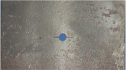 |
594,642 | 7.17 |
| Normal | 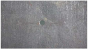 |
560,838 | 6.76 |
| Speckled | 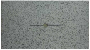 |
885,670 | 10.68 |
The displacement field and crack detection outcomes are depicted in Figure 18. Despite variations in the number of matching point pairs across the different surface textures, all the configurations effectively inferred the displacement field. The influence of matching quantities (or density) will be discussed in Section 3.4.3. The detected crack lengths were 41.7, 42.4, and 41.4 mm with deviations of 5.3%, 3.9%, and 6.1%, respectively. It was evident that the detected crack lengths for all surface textures were reliable, highlighting the reliability of the proposed crack detection method.


3.4.2. ROI Area Ratio
The ROI area ratio is defined as the ratio of the area of ROI to the total area of the image. To evaluate the impact of the ROI area ratio of the image, static tensile tests were conducted at shooting distances of approximately 1, 2, and 3 m, as shown in Figure 19, while the ROI area ratio was 1.00, 0.28, and 0.12, respectively. As the shooting distance increased, the steel plate occupied a smaller area within the entire image. Consequently, the image feature of the same ROI area became much less, which limit the effectiveness of the feature-matching algorithm. Table 3 summarizes the results of feature matching for the steel plate at different shooting distances, while the displacement fields are shown in Figure 20.


| Shooting distance (m) | ROI area ratio | Spatial resolution (mm/pixel) | Number of matching point pairs | Number of matching point pairs/total ROI pixels (%) |
|---|---|---|---|---|
| 1 | 1.00 | 0.0205 | 560,838 | 6.8 |
| 2 | 0.28 | 0.0820 | 124,140 | 5.1 |
| 3 | 0.12 | 0.2000 | 46,098 | 4.6 |


As the shooting distance was extended, the actual length represented by each pixel in the image increased, leading to a decrease in image resolution for the same target area. Furthermore, the ratio of matching point pairs to that in ROI decreased from 6.8% to 4.6% as the ROI area ratio reduced from 1.00 to 0.12.
At the ROI area ratio of 1.00, the displacement cloud clearly depicted abrupt displacement changes due to the presence of the crack, allowing for easy identification of the structural irregularities. However, at the ROI area ratio of 0.28 and 0.12, only the general trend of displacement across the steel plate was observable, with the crack being obscured or indiscernible within the displacement cloud map. This difference highlighted the significance of the ROI area ratio on the level of texture and crack visibility from the displacement analysis.
3.4.3. Density of Matching Point Pairs
The accuracy of the displacement field is significantly influenced by the number of matching point pairs. A sampling of the original matching results at 1%, 5%, 10%, and 50%, corresponding to point pair densities of 0.06%, 0.34%, 0.68%, and 3.4%, respectively, was investigated and the displacement field was inferred based on the sampled data. During the sampling process, n (where n equaled 1, 5, 10, or 50) pairs of matching points were randomly retained for every 100 pairs of matching points on each pair of image patches. Table 4 presents the detailed matching results, while Figure 21 illustrates the y-direction displacement cloud maps.
| Sampling ratio | Number of matching point pairs | Number of matching point pairs/total ROI pixels (%) |
|---|---|---|
| 0.01 | 5608 | 0.06 |
| 0.05 | 28,041 | 0.34 |
| 0.10 | 56,083 | 0.68 |
| 0.50 | 280,419 | 3.40 |


At matching point pair densities of 0.06% and 0.34%, noticeable sawteeth were observed on the inferred displacement cloud maps, leading to failure in the detection of the crack. As the density increased to 0.68% or 3.4% and more matching point pairs were included, the displacement map significantly improved, becoming smoother and closely resembling the original displacement cloud maps. The length of the detected crack on this displacement field also closely matched that of the original displacement field.
3.4.4. Resolution of Input Images
To determine equipment requirements, particularly camera resolution, tests were conducted on images with varying resolutions. Origin images with a resolution of 4k (3840 × 2160) were downsampled to 2k (2560 × 1440), 1080p (1920 × 1080), and 720p (1280 × 720) to simulate different scenarios.
The inferred displacement fields and the detected cracks on images with different resolutions are shown in Figure 22. As the resolution was decreased, the displacement cloud map became rougher and less accurate. The crack length was measured 39.8 mm for 2k images and 41.5 mm for 1080p images, while the crack could not be detected on 720p images. This suggests that the precision slightly dropped when the resolution was decreased from 4k to 2k and 1080p, while 720p image could not be used to detect tiny cracks with a shooting distance of about 1m. Thus, a camera with higher resolution was recommended.

3.4.5. Comparison With Other Crack Detection Approaches
In this section, the proposed method was compared to alternative crack detection approaches, i.e., the Sobel edge extraction operator and the U-Net neural network model. The Sobel and U-Net methods detected the crack directly from a single static image, specifically the image of the steel plate under 150 kN, as illustrated in Figures 23(a) and 23(b), respectively.


For the current data, the Sobel method proved ineffective in detecting the crack as its results were plagued with noise. The U-Net model successfully segmented holes and wire cuttings. However, it failed to detect the crack front at a minuscule scale, which was nearly imperceptible in the image. Consequently, the proposed method demonstrated its superiority in accurately detecting fatigue cracks, offering better performance compared with Sobel and U-Net.
3.4.6. Limitations of the Proposed Method
- 1.
Computing Resource
-
The proposed method requires GPUs with a video memory of 24 GB or larger. Testing has been conducted using two NVIDIA RTX 3090s with two image frames as inputs. The method took 87 s to run, with 70 s dedicated to feature matching, 16 s to displacement field inference, and 1 s to crack detection.
- 2.
Generalization of feature-matching model
-
The trained feature-matching model has been successfully validated on normal, corroded, and speckled steel plates. However, testing under different lighting conditions and on various steel components such as beams, trusses, and bolts has not been conducted, limiting the model’s generalizability, which means the capability of the model in different scenarios.
- 3.
Stability of photographic equipment
-
For the current methodology, it is crucial to ensure the camera was securely fixed on a stable platform during data acquisition. Experiments have revealed that vibrations on the shooting platform adversely impacted feature matching and displacement field inference. If the camera is handheld or mounted on a UAV, additional measures must be taken to compensate for camera motion.
4. Conclusions and Prospect
This research paper presents a visual-based method for inferring displacement fields and detecting tiny fatigue cracks. The approach involved utilizing two frames of the target member under different loading conditions as input data, without the need for processing the member surface. The accuracy of both the inferred displacement field and the detected crack was validated through a series of tensile experiments on steel plates with fatigue cracks. Based on the limited test results, the following observations can be made.
A method for naked-eye invisible fatigue crack detection was proposed, which consisted of three main components, i.e., dense feature matching, displacement field inference, and crack detection. Improvements were made to the feature-matching model, including the model structure, tiled subimages with overlapping regions, and displacement smoothness constraint. An interpolation method was subsequently applied to access the displacement field from the discrete matched points. Finally, the crack was detected based on the discontinuities of displacement around the crack area.
A series of tensile tests on steel plates with fatigue crack propagation were conducted to validate the method, with a special focus on the displacement field and crack length. Compared with the DIC method, the maximum and minimum displacement obtained by the proposed method had a maximum deviation of 13.9%. Compared with the actual crack length, the proposed method had a deviation of 3.9%.
The effects of the surface texture of the steel plate, ROI area ratio, density of matched point pairs, and resolution of input images were discussed. It was found that different surface textures, including normal, speckled, and corroded surfaces, had no significant impact on crack detection. Increased ROI area ratios and density of matched point pairs were helpful for improving the result accuracy. The test case of the ROI ratio of 1.00 performed well, whereas that of 0.28 and 0.12 failed in the crack detection. When the match density in this study was less than 0.68%, sawtooth appeared in the displacement cloud map, which resulted in failure in detecting fatigue crack. The precision of the proposed method slightly dropped when the resolution was decreased from 4k to 2k and 1080p, while 720p image could not be used to detect tiny cracks with a shooting distance of about 1 m.
Currently, only 2D displacement field and crack were detected by the proposed method with the assumption that the ROI was in a plane. Future research will focus on detecting 3D cracks using images collected through binocular vision. In addition, real steel structures experience complex stress states, including tension, compression, shear, bending, and twisting. In this paper, we assessed the method′s feasibility using axial tension, the simplest stress state. Future research will explore the method’s effectiveness under more complex stress conditions.
Conflicts of Interest
The authors declare no conflicts of interest.
Funding
The authors wish to acknowledge the financial support of the National Natural Science Foundation of China (Project No. 52222803), the Early Career Scheme from Hong Kong University Grants Committee (UGC) (Project No. 26209123), and the Fundamental Research Funds for the Central Universities.
Acknowledgments
The authors wish to acknowledge the financial support of the National Natural Science Foundation of China (Project No. 52222803), the Early Career Scheme from Hong Kong University Grants Committee (UGC) (Project No. 26209123), and the Fundamental Research Funds for the Central Universities. The authors would also like to express their sincere gratitude to Mr. Tie-Shan Gao for his assistance during the initial phase of this project. His contributions in literature review, data collection, and experimental setup were essential in laying the groundwork for this research.
Appendix A: Notation List
| Symbol | Shape (in the improved LoFTR model) | Note |
|---|---|---|
| tA | 240, 320 | The input reference image |
| tB | 240, 320 | The input current image |
| , | 128, 120, 160 | The coarse feature map resized tA and tB by CNN |
| , | 128, 120, 160 | The fine feature map resized tA and tB by CNN |
| , | 19200, 128 | Output of the coarse transformer module |
| , | m, 25, 128 (m is the amount of matching point pairs) | Output of the fine transformer module |
| , | m, 2 (m is the amount of matching point pairs) | A matching point pair p on two images |
| dp(, ) | — | Displacement of point p in x- and y-direction |
Open Research
Data Availability Statement
The data are available upon reasonable request.

