Automatic Water Seepage Depth Detection in Concrete Structures Using Percussion Method Combined With Deep Learning Network
Abstract
Water seepage in concrete can significantly degrade the durability of hydraulic concrete structures. Therefore, this paper introduces a new method that combines the percussion method with deep learning techniques to detect the depth of water seepage in concrete structures. Initially, percussion sound signals were collected for different water seepage depths. Then, the proposed one-dimensional convolutional bidirectional gated recurrent unit (BiGRU) network with wide first-layer kernel (1D-WCBGRU) classifies the percussion sound signals for different water seepage depths. The 1D-WCBGRU uses a wide first convolutional kernel to extract features directly from the original percussion signals without the need to extract features manually. Subsequently, the BiGRU is utilized to capture long short-term information from the data, thereby enhancing feature separability and improving the classification accuracy and robustness of the model. Experiments confirm that the 1D-WCBGRU exhibits excellent performance in the seepage depth detection task compared to traditional learning algorithms.
1. Introduction
The use of concrete in buildings is increasingly widespread with the growth of the construction industry. Numerous concrete structures, such as dams, offshore buildings, and marine platforms, have either partial or complete surface exposure to environmental conditions involving water contact [1, 2]. The water permeability of the concrete structure is crucial for its durability, and it is essentially related to the concrete moisture content [3]. Therefore, the internal moisture condition of the concrete component plays a crucial role in determining its serviceability. In addition, moisture in concrete pores results in a variety of physicochemical erosion, such as chloride diffusion [4], steel reinforcement corrosion [5, 6], and alkali–aggregate reactions. Therefore, it is crucial to estimate the variation of moisture within concrete structures. For large-scale hydraulic concrete structures (e.g., dams, bridge abutments, and retaining walls), the water seepage depth is often used as a key indicator of the water content within the concrete [7].
Methods for detecting the depth of water seepage in concrete structures mainly include the capacitance method [8, 9], piezoelectric stress wave method [10, 11], hyperspectral imaging method [12], and microwave method [13], among others. While these methods demonstrate significant potential for detecting water seepage depth in concrete structures, each comes with its own set of limitations. Salt conductivity can adversely impact the capacitance method based on permittivity measurements, leading to inaccuracies in the results [14]. The piezoceramic stress wave method involves the prior installation of sensors in the structure, which may increase the cost and reduce the structural load-bearing capacity. Hyperspectral imaging methods may damage the specimen and require the involvement of specialized personnel. The accuracy of the microwave method is compromised at times due to internal scattering and diffraction arising from the heterogeneity of concrete. Hence, there is a need to identify a straightforward and cost-effective method for detecting the water seepage depth in concrete structures.
The percussion method can be utilized to gather information about potential damage by striking the surface of a test object. It is gaining prominence in nondestructive testing (NDT) due to its ease of operation, cost-effectiveness, and ability to function without sensors requiring direct contact with the object [15–18]. Researchers focusing on the percussion method were primarily concerned with the structural vibration response induced by percussion rather than the sound generated by the impact [19]. However, with the swift advancement of machine learning (ML) techniques, there is a growing interest among researchers in sounds induced by percussion. Chen et al. [20] extracted power spectrum density (PSD) energy from percussion sound signals as features and employed a support vector machine (SVM) algorithm to classify subsurface voids in CFST structures. Zheng et al. [21] converted percussion sound signals with different concrete water content into Mel-frequency cepstral coefficients (MFCCs) and classified them using the SVM algorithm. Cheng et al. [16] demonstrated the effectiveness of the percussion method for detecting pipeline deposits by employing the SVM algorithm to identify the MFCC extracted from percussion sound signals. He et al. [22] used the K-nearest neighbors (KNNs) algorithm to recognize PSD features extracted from percussion sound signals. This was applied to detect the looseness condition in underwater bolted connections. Thus, to establish the connection between structural damage (e.g., loose bolts) and percussion-induced sound signals, the mentioned percussion methods heavily depend on ML techniques. However, ML techniques require features to be manually crafted and then input into the classifier. This approach might overlook critical features in percussion-induced sound signals, resulting in suboptimal classification accuracy [23]. Furthermore, the antinoise capacity and adaptability of existing ML techniques remain unverified, thereby constraining their practical effectiveness in real-world scenarios [24].
Recently, deep learning (DL) techniques have advanced rapidly, emerging as a promising solution to tackle the aforementioned challenges. In contrast to traditional ML techniques, DL techniques can autonomously extract features from data without the need for manual feature extraction. As a typical DL algorithm, convolutional neural networks (CNNs) have gotten a lot of attention because of their superior performance. Chuang, Tsai, and Wang [25] utilized CNNs to classify Mel-frequency spectrograms obtained by transforming one-dimensional signals for water pipe leak detection. Yuan et al. [26] employed CNNs to implement bolt-loosening detection by classifying Mel spectrograms derived from one-dimensional signals. However, when traditional CNNs process one-dimensional data such as audio, it is often necessary to convert the data into two-dimensional images, which can lead to redundant computations. To address this issue, researchers have introduced one-dimensional CNNs (1D-CNNs). Abdeljaber et al. [27] realized damage detection and real-time damage localization based on vibration by fusing feature extraction and classification modules into a compact learning body using 1D-CNN. Eren [28] employed 1D-CNN for rapid identification of bearing faults. In addition, 1D-CNN has been widely studied in pipeline leakage and water deposition detection [29, 30], bolt loosening detection [31, 32], intelligent diagnosis of rotating machinery [33], etc. However, to the best of the author’s knowledge, no existing research has applied DL techniques in combination with the percussion method to detect the depth of water seepage in concrete structures.
This paper presents a framework for detecting water seepage depth through the application of a percussion-based DL technique. The suggested DL framework is termed as the one-dimensional convolutional bidirectional gated recurrent unit network (1D-WCBGRU) with a wide first kernel. This hybrid framework combines the 1D-CNN and bidirectional gated recurrent unit (BiGRU). Unlike traditional ML/DL techniques, this framework harmonizes the potent feature extraction capability of 1D-CNN with BiGRU’s ability to capture both long-temporal and short-temporal relationships in features. This combination enhances the accuracy and robustness of predicting concrete structure water seepage depth.
This paper’s main contributions are as follows: (1) This paper establishes a finite element model to simulate the water seepage depth in concrete structures and verifies the feasibility of detecting water seepage depth using the percussion method. Additionally, a DL model is proposed, primarily for classifying percussion sound signals to achieve the detection of water seepage depth. (2) To enhance the feature extraction capability of the 1D-WCBGRU model, we designed a wide kernel convolutional block to extract more representative features from the original signal. The model also integrates a BiGRU block to bolster predictive performance, thereby improving the model’s accuracy in classifying percussion sound signals. (3) The experimental results demonstrate that the 1D-WCBGRU model exhibits strong noise immunity in noisy environments and shows powerful adaptability across various application conditions, proving the model’s potential and effectiveness in practical applications.
The rest of the paper is organized as follows. Section 2 provides an explanation of the model’s theoretical background. A detailed description of the 1D-WCBGRU model is provided in Section 3. In Section 4, the experimental setup is described in detail. In Section 5, we compare the performance of 1D-WCBGRU with other methods. Section 6 summarizes the study.
2. Theoretical Background
2.1. 1D-CNNs
In recent years, CNNs which are the most classical DL networks have attracted a lot of attention due to their excellent feature extraction and powerful fitting ability [34]. While CNNs have demonstrated remarkable proficiency in computer vision tasks like image classification [35], they face challenges in directly classifying 1D data. Various investigations [36, 37] attempted to convert 1D data into 2D images using different techniques, enabling CNNs to classify 1D data. However, this approach often results in redundant computations. To effectively address the above drawbacks, researchers [38] proposed that feature extraction and classification can be performed directly on 1D data using 1D-CNN. The traditional 1D-CNN has five main components: convolutional layer, activation layer, pooling layer, fully connected (FC) layer, and Softmax function output layer.
2.2. Gated Recurrent Unit (GRU)
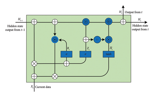
2.3. Numerical Simulation
Zhou et al. [17] investigated the correlation between percussion-induced vibration and percussion sound by wavelet packet decomposition and sound reconstruction techniques. Therefore, the sound produced by percussing concrete varies in response to the vibrations induced by the impact.
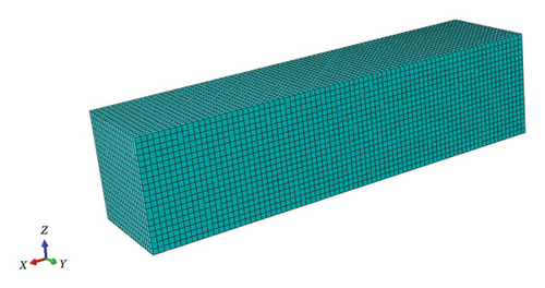
Luo and Yang [45] conducted experiments demonstrating that changes in the natural frequency of a structure influence its vibrational characteristics, resulting in distinct percussion sounds. Thus, numerical simulations were conducted for six concrete specimens with varying water seepage depths using the commercial finite element software Abaqus in this study. An example finite element model of a concrete specimen with dimensions 100 mm × 100 mm × 400 mm is illustrated in Figure 2. In this paper, the impact of water seepage depth on resonance frequency was simulated by adjusting the modulus of elasticity of concrete at different heights (0 mm, 80 mm, 160 mm, 240 mm, 320 mm, and 400 mm). All parameters were held constant except for the varying of the modulus of elasticity.
2.3.1. Concrete Constitutive Model
2.3.2. Boundary Conditions and Mesh Sizes
The model simulates a portion of a mass hydraulic concrete structure with column top displacements (Ux, Uy, and UZ) and column bottom displacements (Ux, Uy, and UZ) in all three directions constrained to 0. At the same time, the rotational degrees of freedom (URx, URy, and URz) of the column was 0. The concrete mesh size was set to 5 mm.
The concrete model was subjected to modal analysis to validate the effect of seepage depth on the natural frequency of concrete. Table 1 illustrates the first three orders of natural frequency for concrete specimens at different water seepage depths. The results indicate that the increase in the depth of water seepage leads to a gradual increase in the first three orders of the natural frequency of the concrete specimens. Thus, with other conditions held constant, the sound generated from percussion is influenced by the water seepage depth, confirming the feasibility of using percussion sound to identify the water seepage depth in concrete structures.
| Water seepage depth (mm) | First mode frequency (Hz) | Second mode frequency (Hz) | Third mode frequency (Hz) |
|---|---|---|---|
| 0 | 1627.4 | 2492.1 | 3597.1 |
| 80 | 1646.1 | 2523.8 | 3633.8 |
| 160 | 1652.6 | 2538.2 | 3656.2 |
| 240 | 1662.6 | 2539.6 | 3671.8 |
| 320 | 1669.6 | 2552.5 | 3694.0 |
| 400 | 1688.8 | 2586.1 | 3732.8 |
3. Proposal Method
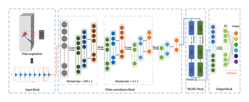
This paper introduces a novel deep neural network designed to address the classification of percussion sounds corresponding to different water seepage depths. Figure 3 illustrates the proposed 1D-WCBGRU architecture, which mainly consists of an input block, a wide kernel convolutional block, a BiGRU block, and an output block. The detailed parameters of the 1D-WCBGRU are shown in Table 2. The fundamental mechanism involves feeding percussion sound signals from various water seepage depths into the 1D-WCBGRU. First, a wide convolutional kernel (kernel size = 256) extracts local features from the audio signals. To reduce the computational complexity and dimensionality of the feature maps, the output of the convolutional layer is subjected to max pooling operation. Subsequently, a smaller convolutional kernel (kernel size = 2) is employed for a secondary convolution operation to further extract features from the audio signals. Concurrently, to enhance the model’s training stability and generalization capability, layer normalization (LN) is introduced, thereby improving the model’s adaptability to different input distributions. Following this, BiGRU is incorporated to more effectively capture contextual information within audio sequences. After passing through this layer, the model uses a global average pooling (GAP) layer to map audio sequences of varying lengths to a fixed-length vector. This operation enables the model to better handle audio inputs of different lengths, reduces the number of model parameters, and mitigates the risk of overfitting. Finally, the model employs an FC layer to map audio features to the output layer. The Softmax function is employed to provide for probabilistic output across six categories, achieving accurate classification of different types of damage. The model effectively captures multilevel information from audio signals, thereby enhancing the model’s classification performance and robustness. The theoretical background of each module is described in the following section.
| Layer | Parameter settings |
|---|---|
| Conv1d_1 | Filers = 32, kernel_size = 256, and stride = 1, activation = ReLU |
| Maxpool1d_1 | Kernel_size = 2 |
| Conv1d_2 | Filers = 64, kernel_size = 2, and stride = 1, activation = ReLU |
| Maxpool1d_2 | Kernel_size = 2 |
| LayerNorm | Normalized_shape = 64 |
| GRU | Input_size = 64 and hidden_size = 32, bidirectional = ture |
| Global average pooling 1D | Out_size = 1 |
| FC | In_features = 64 and out_features = 6 |
3.1. Wide Kernel Convolutional Block
Researchers [48] discovered that the size of the convolutional kernel significantly impacts the extracted features when using the same quantity of input samples. The challenge arises because using a model with small kernels for one-dimensional audio signals results in a very deep network, which is difficult to train and thus not practical. In addition, the small kernel in the first layer is prone to interference from high-frequency noise. Therefore, the first convolutional layer utilizes a wide kernel to effectively capture the complexities of low-frequency signals for feature extraction. After that, employing small kernels aids in obtaining a good representation of the input signal, thereby enhancing network performance. Note that the depth of the network is further increased by applying the ReLU activation function after each convolutional operation.
3.2. Bidirectional GRU
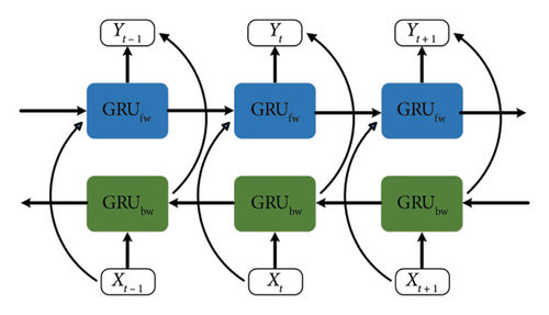
3.3. Output Block
4. Experimental Setup
Three concrete prismatic specimens, each with dimensions of 100 mm × 100 mm × 400 mm were fabricated and tested in a laboratory setting to validate the proposed method. The concrete was designed to have a compressive strength of 30 MPa. The mix ratio for achieving this strength is presented in Table 3.
| Component | Water | Cement | Coarse aggregate | Fine aggregate | Superplasticizer |
|---|---|---|---|---|---|
| Quantity (kg/m3) | 183 | 450 | 1192 | 600 | 5 |
Following a curing period of 28 days under standardized conditions, the concrete specimens were subsequently dried in an oven at 105°C for 48 h, ensuring that their mass reached a constant value. Once the concrete had cooled completely, the specimens were immersed in pure water at the specified depth for about 4 h. After that, the concrete specimens were taken out of the water and dried with a cloth until no water droplets remained on the surface, after which the percussion test was conducted. Given the short duration of the percussion experiments, it was assumed that water seepage depth inside the concrete remained constant. Figure 5(a) illustrates the experimental samples and equipment.
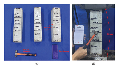
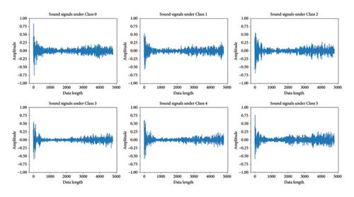
A total of six different damage conditions were set up for the experiment, and each damage condition was assigned a label value from 0 to 5, as shown in Table 4. The apparatus used for the hammering experiment comprised an impact hammer and a smartphone. Throughout the experiment, the specimen was secured at both ends using the fixture to prevent disturbances caused by the concrete shaking during percussion. As depicted in Figure 5(b), the fixture was in contact with the concrete specimen and applied no force. Concrete was percussed at specified locations 100 times with uniform force to produce an audio signal. Simultaneously, the audio signal was captured at a sampling rate of 48 kHz by a smartphone situated 100 mm from the percussion point, as depicted in Figure 5(b). The experiment was performed in a quiet laboratory to minimize noise disturbance. Afterward, the audio signal was preprocessed by converting the dual-channel raw audio to a single channel with a sampling time set to 0.1 s (i.e., a sample length of 4800). Peak points are sample points in the waveform where the amplitude exceeds a predefined threshold of 15,000. These peak points serve as the starting point for each percussion signal. To ensure an accurate separation of each individual knock sample, a minimum gap was introduced between two consecutive peak points, allowing only one peak point to be selected within this gap. Finally, the individual percussion raw signals were normalized and used as inputs to the model. Figure 6 illustrates a portion of the percussion sound signals waveform captured at various water seepage depths.
| Label | Water depth (mm) | Sampling number |
|---|---|---|
| 0 | 0 | 100 |
| 1 | 80 | 100 |
| 2 | 160 | 100 |
| 3 | 240 | 100 |
| 4 | 320 | 100 |
| 5 | 400 | 100 |
5. Results and Discussion
5.1. The Model Training
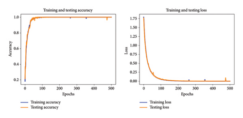
The accuracy and loss curves stabilize after small fluctuations during 500 epochs of training, as shown in Figure 7. Throughout the training process, the close alignment of the training and test curves indicates that the model has strong generalization ability. The model achieves 100% training accuracy and 100% test accuracy after 500 epochs of training. This confirms the sensitivity of the 1D-WCBGRU to water seepage depth in concrete structures, showcasing its effective feature extraction and learning capabilities during training. Simultaneously, the 1D-WCBGRU has superior performance on unseen datasets.
5.2. Methodology Comparison
| Method | PSD + DT | MFCC + SVM | MFCC + CNN | 1D-WDCNN | 1D-ResNet | 1D-WCBGRU |
|---|---|---|---|---|---|---|
| Accuracy | 0.7926 | 0.9722 | 0.9815 | 0.9907 | 0.9926 | 1.0000 |
| Precision | 0.7967 | 0.9730 | 0.9815 | 0.9909 | 0.9928 | 1.0000 |
| Recall | 0.7926 | 0.9722 | 0.9815 | 0.9907 | 0.9926 | 1.0000 |
| F1-score | 0.7932 | 0.9730 | 0.9815 | 0.9906 | 0.9926 | 1.0000 |
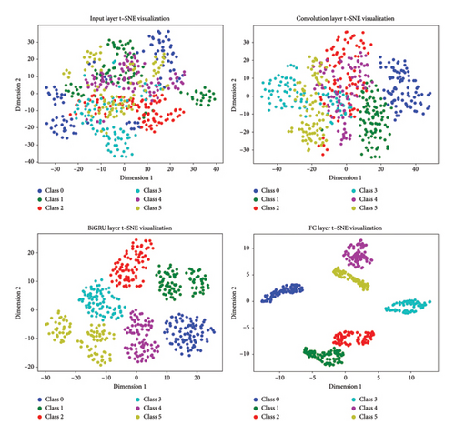
The t-distributed stochastic neighbor embedding (t-SNE) technique is employed to generate a 2D visual representation of the feature mapping. This approach enhances the understanding of the features learned by the model and facilitates the analysis of the model’s representation in the data space. The 2D visualization results of the feature mapping for the input layer, convolutional layer, BiGRU layer, and FC layer of the 1D-WCBGRU are obtained using t-SNE, as illustrated in Figure 9. In this figure, each point represents a data sample, and the six different colored points correspond to the six categories of water seepage depths. The 2D visualization results from the input layer indicated a significant superposition of data points from different categories, making it challenging to differentiate the feature information of the original data. In the convolutional layer, while no clear clustering of points is observed for each category, their distribution becomes progressively more structured and organized. In contrast, features are more distinguishable after the BiGRU layer, with only a few instances of misclassification. This is evidence that the BiGRU layer enhances feature distinguishability. Ultimately, the features are perfectly classified after the FC layer. Overall, the coordinated interaction of the individual blocks significantly enhances the feature extraction capability of the 1D-WCBGRU model.
5.3. Adaptability Test
Despite the outstanding performance exhibited by the 1D-WCBGRU in the aforementioned experiments, certain challenges persist in practical applications. For this reason, two experiments were designed in this section to test the adaptability of the 1D-WCBGRU.
5.3.1. Effect of Percussion Position
Liu et al. [53] investigated the correlation between the location of percussion and detection effectiveness. The detection accuracy decreases as the percussion position moves farther away from the bolt. This could be attributed to the further distance between the percussion positions and the defect, which introduces greater physical separation and structural differences. As a result, more irrelevant information is captured, leading to a decrease in detection accuracy. In practice, it is difficult to determine the approximate range of water seepage depth to select the appropriate percussion position. Therefore, the experiment was designed with different percussion positions (120 mm and 280 mm) to assess the adaptability of the 1D-WCBGRU. Table 6 depicts the accuracy of each model in classifying the water seepage depth at different percussion positions. The results demonstrate the superiority of the proposed 1D-WCBGRU model compared to the other methods.
| Percussion position (mm) | Methods | |||||
|---|---|---|---|---|---|---|
| PSD + DT | MFCC + SVM | MFCC + CNN | 1D-WDCNN | 1D-ResNet | 1D-WCBGRU | |
| 120 | 0.6944 | 0.9593 | 0.9889 | 0.9851 | 0.9833 | 0.9981 |
| 280 | 0.7360 | 0.9644 | 0.9850 | 0.9925 | 0.9831 | 1.0000 |
5.3.2. Cross-Dataset Performance Evaluation
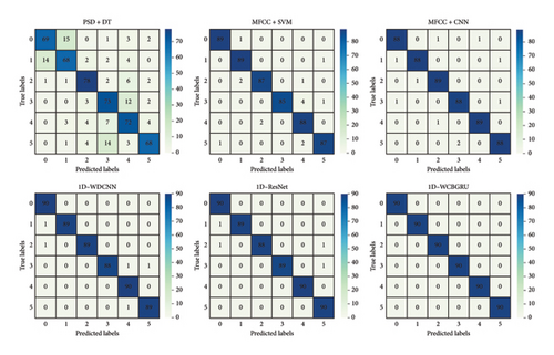
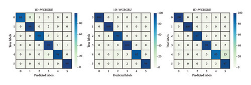
As concrete is an inhomogeneous multiphase composite material, the audio features captured through the percussion method may vary even for concrete with identical mix ratios, due to differences in the manufacturing process. Consequently, additional investigations into the adaptability of the proposed model are warranted. For this purpose, the two datasets are merged into a training set, and the other dataset is used as a test set. This indicates that the training and test sets were derived from separate concrete samples, ensuring no overlap between the datasets. Table 7 demonstrates the accuracy of each method. Figure 10 depicts the classification results for the 1D-WCBGRU across different percussion positions in the cross-dataset. It is worth noting that when considering cross-dataset, the accuracy of all methods tends to decrease. However, the 1D-WCBGRU consistently outperforms the other methods.
| Percussion position (mm) | Methods | |||||
|---|---|---|---|---|---|---|
| PSD + DT | MFCC + SVM | MFCC + CNN | 1D-WDCNN | 1D-ResNet | 1D-WCBGRU | |
| 120 | 0.2883 | 0.3967 | 0.3967 | 0.6717 | 0.4800 | 0.9450 |
| 200 | 0.2450 | 0.4117 | 0.3817 | 0.6417 | 0.5450 | 0.9767 |
| 280 | 0.3650 | 0.4617 | 0.2217 | 0.5600 | 0.6783 | 0.9617 |
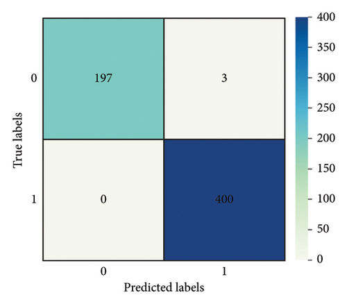
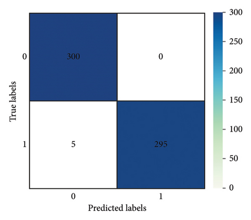
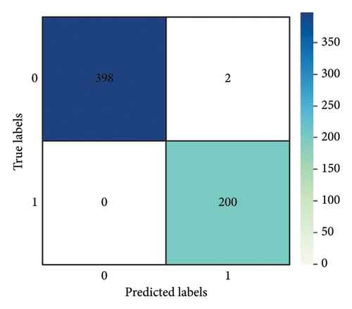
In real-world scenarios, the depth of water seepage in concrete structures is constantly changing and may differ from the preset depths used in this experiment, potentially making detection more challenging. To address this concern, the confusion matrix depicted in Figure 10 was simplified in Figure 11 by focusing solely on the relative position of the water seepage depth to the percussion positions. In Figure 11, the label “0” represents instances where the water level height is below the percussion positions, while the label “1” indicates instances where the water level height is above the percussion positions. The accuracy of the 1D-WCBGRU at percussion positions of 120 mm, 200 mm, and 280 mm is 99.50%, 99.17%, and 99.67%, respectively. This demonstrates that the 1D-WCBGRU achieves high accuracy when the relative position of the percussion to the water seepage depth is the primary consideration.
To further evaluate the performance of the 1D-WCBGRU on unseen datasets, additional experiments were conducted based on the water seepage depth and the relative positions of percussion. The data labels “0,” “2,” “3,” and “5” in the training set were used to generate a new training set, and the data labels “1” and “4” in the test set were used to generate a new test set. In the new training set, data labeled “0” and “2” were combined into label “0,” while data labeled “3” and “5” were consolidated into label “1.” In the new test set, “0” and “1” correspond to labels “1” and “4” in the original test set, respectively. It should be noted that only the data from the 200-mm percussion position have been selected for the purpose of balancing the data. The classification accuracy is shown in Table 8. Notably, the 1D-WCBGRU still has high classification accuracy cross-dataset for uncollected water seepage depth signals.
| Methods | PSD + DT | MFCC + SVM | MFCC + CNN | 1D-WDCNN | 1D-ResNet | 1D-WCBGRU |
|---|---|---|---|---|---|---|
| Accuracy | 0.8000 | 0.5700 | 0.5300 | 0.6900 | 0.6350 | 0.9550 |
5.4. Model Performance in Noisy Environment
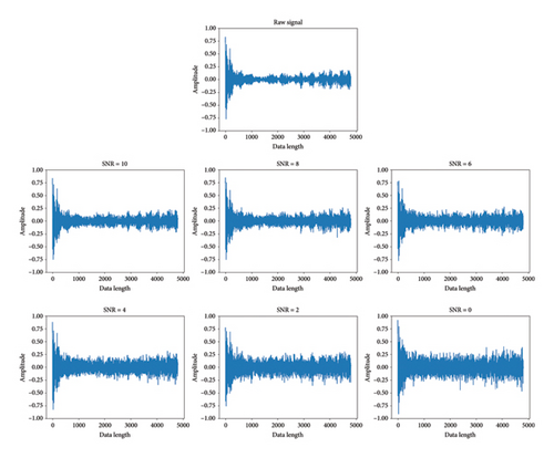
Figure 13 provides a visualization of the classification accuracy in a noisy environment for different percussion positions cross-dataset. The combined analysis shows that the accuracy of all methods decreases in noisy environments, underscoring the general adverse effect of noise on model performance. Three feature extraction methods (PSD + DT, MFCC + SVM, and MFCC + CNN) perform poorly in noisy environments. However, the three methods (1D-WDCNN, 1D-ResNet, and 1D-WCBGRU) that directly take 1D audio signals as inputs show better performance. This indicates that the direct use of 1D signals as input facilitates the capture and retention of key features in the audio data. Notably, the 1D-WCBGRU has better noise immunity.
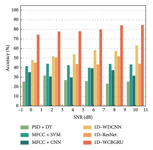
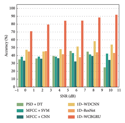
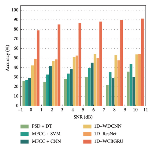
In addition, it can be observed from the figure that the accuracy of some models instead increases after adding Gaussian white noise. For instance, 1D-ResNet’s classification accuracy increased by 3.83% after introducing Gaussian white noise with an SNR of 8 to the data collected at a 120-mm percussion position, compared to using noiseless data. This phenomenon may result from the model overfitting specific features in the training set that were absent in the test set. When noise was introduced into the data, these overfitted features were masked by the noise, making the model rely on more general and robust features. However, the 1D-WCBGRU model does not suffer from this problem, indicating that the model has been effective in avoiding the overfitting problem in the absence of noise.
5.5. Ablation Experiment
The 1D-WCBGRU model utilizes 1D-CNN as the model skeleton, the first layer of the convolutional kernel was designed as a wide kernel convolutional block, and a BiGRU block is applied. To evaluate the effectiveness of these enhancements for audio recognition, a series of ablation experiments were conducted. In these experiments, the improved components were sequentially removed, starting with the BiGRU block, until the model reverted to the base 1D-CNN architecture. Then recovery of the BiGRU block was started and finally restored to the 1D-WCBGRU model. Each modification was individually removed, followed by retraining and retesting the model using both the standard dataset and the cross-dataset data collected at a percussion depth of 200 mm to assess the effectiveness of each module, with results presented in Table 9.
| Wide kernel | BiGRU | Standard dataset | Cross dataset |
|---|---|---|---|
| 0.9963 | 0.8150 | ||
| √ | 0.9981 | 0.8633 | |
| √ | 1.0000 | 0.8833 | |
| √ | √ | 1.0000 | 0.9767 |
The results show that both the wide convolutional kernel and the BiGRU block contribute remarkably to improving the accuracy of the model. While the results derived solely from the standard dataset may indicate that the incorporation of wide kernel convolutional block and BiGRU block into the model does not significantly improve accuracy, the inclusion of these two modules considerably augments the model’s feature extraction capabilities. This enhancement is particularly vital when addressing more complex datasets, as it empowers the model to generalize and adapt to diverse data distributions with greater efficacy. The significance of these two modules becomes particularly evident in the cross-dataset scenario. Since the training data and test data are derived from different specimens, the model must possess stronger generalization capabilities to ensure reliable performance across varying datasets. In this case, the wide convolutional kernel and the BiGRU blocks improve the accuracy by 6.83% and 4.83%, respectively, and the synergistic effect of the two improves the accuracy by 16.17%. The inclusion of the wide convolutional kernel and the BiGRU block significantly enhances the model’s generalization ability.
6. Conclusion
- 1.
The experiments confirm the feasibility of using the 1D-WCBGRU for water seepage depth detection. The 1D-WCBGRU achieves a classification accuracy of 100%.
- 2.
Experiments cross-datasets and different percussion locations demonstrate the superiority of the 1D-WCBGRU in water seepage depth detection. In addition, the 1D-WCBGRU accurately predicts the relative position of the water level to the percussion point even when the seepage depth is not considered.
- 3.
The 1D-WCBGRU demonstrates robust noise immunity when tested with audio data containing added noise. In comparison with other methods, the model maintains a stable performance in noisy environments.
- 4.
The t-SNE technique and ablation experiments confirm that the introduction of the wide convolutional kernel and the BiGRU block provides the 1D-WCBGRU with favorable feature separability and generalization ability.
Overall, the 1D-WCBGRU shows promise as a reliable method for water seepage depth detection, given its superior performance demonstrated in the task of water seepage depth detection.
Conflicts of Interest
The authors declare no conflicts of interest.
Author Contributions
Wenjie Huang: conceptualization, methodology, writing–original draft preparation. Kai Zhou: formal analysis, writing–original draft preparation, funding acquisition. Jicheng Zhang: investigation, resources, writing–original draft preparation. Longguang Peng: investigation, resources, software, data curation. Guofeng Du: methodology, writing–review and editing, funding acquisition. Zezhong Zheng: conceptualization, methodology, writing–review and editing.
Funding
This research was financially supported by the National Natural Science Foundation of China (Grant No. 52078052 and 12302164).
Acknowledgments
The authors thank the National Natural Science Foundation of China (No. 52078052 and No. 12302164) for financial support.
Open Research
Data Availability Statement
The data used to support the findings of this study are available from the corresponding author on request.


