Detection of Rupture Damage Degree in Laminated Rubber Bearings Using a Piezoelectric-Based Active Sensing Method and Hybrid Machine Learning Algorithms
Abstract
Laminated rubber bearings may exhibit rupture damage due to factors such as temperature variations and seismic activity, which can reduce their isolation performance. Current detection methods, including human-vision inspection and computer-vision inspection, have certain limitations in accurately assessing the degree of rupture damage. This study attempts to combine the piezoelectric-based active sensing method with a machine learning algorithm to detect rupture damage in laminated rubber bearings. A series of laminated rubber bearings with varying degrees of rupture damage were fabricated, and 1440 sets of detection signals were obtained through experiments using the active sensing method. This study proposes a hybrid machine learning algorithm that integrates a one-dimensional convolutional neural network (1DCNN), long short–term memory (LSTM) network, Bayesian optimization (BO) algorithm, and extreme gradient boosting (XGB) algorithm. The algorithm involves using the 1DCNN and LSTM algorithms to extract the deep features from the wavelet packet energy spectra of the detection signals, and then employing the XGB algorithm optimized by the BO algorithm to construct the prediction model. The research results indicate that the proposed 1DCNN–LSTM–BO–XGB model achieved an accuracy value of 98.6% on the test set, outperforming the 1DCNN–LSTM (91.7%), 1DCNN (88.9%), LSTM (25.0%), XGB (90.3%), and SVM (66.7%) algorithms. Therefore, the combination of the active sensing method and machine learning algorithm shows promising application prospects in detecting the degree of rupture damage in laminated rubber bearings.
1. Introduction
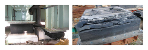
In the fields of building engineering and bridge engineering, laminated rubber bearings are widely used due to their excellent seismic isolation performance, cost-effectiveness, and durability [1, 2]. Laminated rubber bearings effectively reduce the seismic response of structures by absorbing and dissipating seismic energy, thereby ensuring the stability and safety of the structure. However, with increased service time, changes in environmental factors, and seismic actions, laminated rubber bearings are inevitably prone to rupture damage (as shown in Figure 1) [3]. For example, on September 5, 2022, a 6.8 magnitude earthquake occurred in Luding County, Ganzi Prefecture, Sichuan [4]. Several laminated rubber bearings were found to have ruptured and damaged. Such damage can degrade the mechanical performance of the bearings, particularly the horizontal shear stiffness, thus posing a safety risk to the structure. Therefore, it is essential to detect whether laminated rubber bearings have suffered rupture damage and to assess the degree of the damage.

Current detection methods, including human-vision inspection and computer-vision inspection [6], have certain limitations in identifying rupture damage in laminated rubber bearings. For human-vision inspection, the process primarily relies on the inspectors’ experience, which introduces potential errors and variability influenced by the inspectors’ expertise. In addition, laminated rubber bearings often bear significant axial pressure, causing the crack surfaces to be compressed, which complicates the accurate quantification of rupture damage. Moreover, when bearings are located in unfavorable positions, such as confined spaces or elevated locations, inspectors face challenges in getting close enough for effective inspection. On the other hand, computer-vision inspection involves capturing images of the bearings using cameras, drones, and other devices, followed by the application of artificial recognition and deep learning techniques to identify the condition of the laminated rubber bearing. For example, Cui et al. [6] combined computer-vision inspection with deep learning (i.e., convolutional neural network [CNN]) to achieve the precise classification of three types of laminated rubber bearing conditions (i.e., normal condition, severe cracking and voids, and shearing over the limit). However, this approach has several drawbacks. The large number of laminated rubber bearings dispersed across different locations requires extensive deployment of cameras, leading to high costs. Furthermore, drone operations are significantly affected by environmental conditions and the positioning of the bearings, making it challenging to accurately assess the degree of rupture damage. In recent years, Zeng et al. [7] successfully applied the piezoelectric-based active sensing method to full-scale laminated rubber bearing rupture damage detection, demonstrating the method’s feasibility. However, due to the uncontrollability of the damage creation process, the damage degree was limited to only two levels: normal and complete rupture. Therefore, this study further explores the fabrication of bearings with multiple damage degrees and the development of a high-precision damage detection model.
However, the relationship between the detection signals and the degree of rupture damage is complex, posing challenges to the accurate identification of the damage degree. Machine learning technology, known for its excellent performance in modeling complex engineering problems, offers a new solution. For example, Zhang, Liu, and Zhao [8] combined CNNs with machine vision and proposed a new structural displacement monitoring method, achieving a correlation coefficient of 0.984 between the monitoring results and those of a laser displacement sensor. Le-Xuan, Bui-Tien, and Tran-Ngoc [9] integrated one-dimensional CNN (1DCNN), long short–term memory (LSTM) networks, and residual networks (ResNets) to propose a deep learning method capable of accurately detecting bridge structural damage based on transient data processing, achieving an accuracy of 81.5%. Therefore, this paper attempts to establish a highly accurate rupture damage detection model using machine learning techniques, thereby enhancing the accuracy and reliability of the detection process. In damage detection, feature extraction from the detection signals is a crucial step. Currently, well-known algorithms for handling time series data include 1DCNN and LSTM. 1DCNN extracts local features from time series data based on one-dimensional convolution, enabling the recognition of continuous data patterns and feature changes in time series without relying on window size or stride [9]. Abdeljaber et al. [10] applied 1DCNN to structural damage detection based on vibration signals and found that 1DCNN possesses the ability to automatically extract optimal features from raw data, achieving a high level of generalization. LSTM is a special form of recurrent neural network (RNN), with the advantage of retaining and processing information over extended periods, allowing the model to recognize and memorize gradually changing patterns between data points across different time steps [11, 12]. For example, Zhang and Zhou [13] proposed a new anomaly detection method for bridge vibration data based on CNN and LSTM, achieving an average accuracy of over 94% in the automatic classification task of continuous monitoring data over 42 days on a long-span bridge. In the proposed method, CNN is used to extract local high-level features from the input sequence, while LSTM further learns its global long-term dependencies. Therefore, this paper first uses wavelet packet decomposition (WPD) to decompose the detection signals into different frequency and time scales, then applies 1DCNN to identify local features of the signals in the frequency domain, and finally, uses LSTM to capture the temporal dependencies of the signals. By extracting deep features from the multiscale wavelet packet energy spectra through the 1DCNN–LSTM, a more refined high-dimensional feature vector can be generated, which improves the feature discrimination between different categories, thereby enhancing the performance of the detection model.
The extreme gradient boosting (XGB) algorithm is known for its efficiency, robustness, and excellent predictive performance, making it particularly suitable for handling large-scale and complex datasets, and it has been widely applied across various fields [14, 15]. For example, Sun, Zhang, and Zhang [14] applied the XGB algorithm to the classification task of well logging fluid in the oil and gas exploration field, achieving a classification accuracy of 96%. However, manually adjusting the hyperparameters of the XGB model has some problems such as low efficiency and poor accuracy. Therefore, in this paper, while using the XGB algorithm to process the extracted features, the Bayesian optimization (BO) algorithm is also employed to determine the optimal hyperparameters of the XGB model, aiming to establish a highly accurate damage degree prediction model in a more efficient manner.
Therefore, the novelty and contributions of this study are mainly reflected in the following points: (1) A total of 1440 detection signals from laminated rubber bearings with six degrees of rupture damage were collected through experiments using the active sensing method and (2) a new hybrid algorithm integrating 1DCNN, LSTM, BO, and XGB was proposed, and a rupture damage detection model with a test set accuracy as high as 98.6% was developed.
The structure of this paper is as follows. Section 2 introduces the specimens and experimental scheme. Section 3 presents the experimental results. Section 4 elucidates the rupture damage detection method based on the 1DCNN–LSTM–BO–XGB algorithm and provides a brief introduction to the relevant algorithms. Section 5 describes the modeling process and prediction results of the proposed rupture damage detection model and compares it with other machine learning models. Section 6 presents the conclusions of the study.
2. Brief Introduction of the Experiment
2.1. Specimen
2.1.1. Smart Bearing Construction
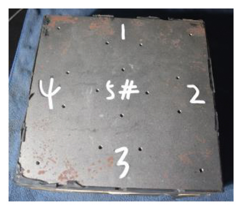
As shown in Figure 2, the smart bearing used in this study mainly consists of eight transducers, eight cover plates, two protective steel plates, and a laminated rubber bearing. To ensure that the placement of the transducers does not affect the axial and horizontal stiffness of the bearing, the transducers are symmetrically arranged on the upper and lower sides of the bearing. The upper transducers are used to generate the excitation signal (exciters), while the lower transducers are used to collect the detection signal (sensors). The purpose of placing a cover plate is to apply a certain pressure to the transducer, ensuring the effectiveness of wave transmission. The primary purpose of placing protective steel plates on the upper and lower sides of the bearing is to ensure that the transducers do not come into direct contact with the upper and lower structures (as the transducers can withstand only limited axial pressure), thereby allowing them to function properly. Each protective steel plate is designed with four measurement holes (to accommodate the transducers), four wire ducts (to house the connecting wires), and multiple bolt holes.
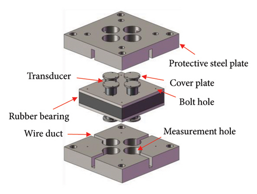
As shown in Figure 2(a), there are four exciters (G1–G4) and four sensors (S1–S4) arranged on the upper and lower sides of the bearing, respectively. In this study, the transducers used are longitudinal wave transducers with a diameter of 38 mm and a height of 30 mm. The specific parameters are shown in Table 1.
| Resonant frequency (kHz) | Dielectric constant | Piezoelectric constant | Impedance (Ω) |
|---|---|---|---|
| 58 | 1700 | 190–450 pC/N | 1900 |
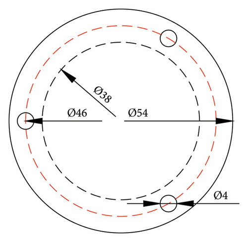
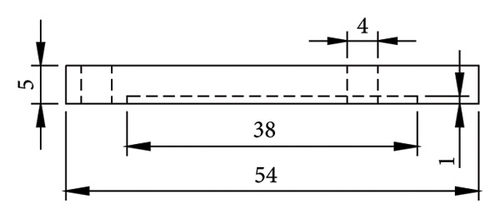
As shown in Figure 2(a), the transducer is placed between the cover plate and the bearing, and a certain amount of pressure (with a torque value of 2.5 N·m each) is applied to the cover plate using a bolted connection, thereby fixing the transducer to the surface of the bearing. The bolts connecting the transducers and the bearing are cup head hex socket bolts with a diameter of 4 mm and a length of 40 mm, with a strength grade of 12.9 (tensile strength of 1200 MPa and yield strength of 1080 MPa). As shown in Figure 3, the cover plate has a diameter of 54 mm and a thickness of 5 mm, with a groove of 38 mm in diameter and 1 mm in depth (used for mounting the transducers and maintaining its relative position to the cover plate). The three bolt holes are evenly spaced, with each located 46 mm from the center of the cover plate.
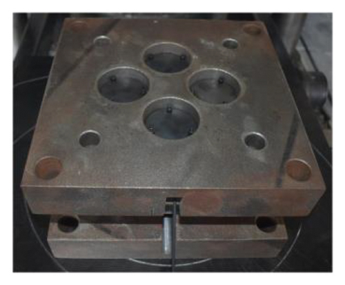
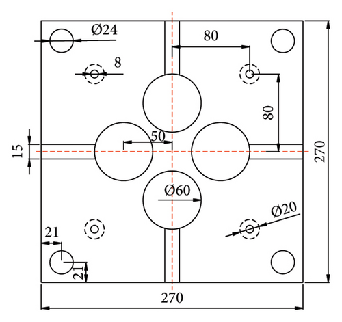
As shown in Figure 4, the protective steel plate has dimensions of 270 mm (length) × 270 mm (width) × 50 mm (height). The internal measurement hole has a diameter of 60 mm, with a distance of 50 mm between its center and the center of the protective steel plate.

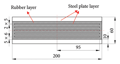
As shown in Figure 5, the square laminated rubber bearing has dimensions of 200 mm (length) × 200 mm (width) × 60 mm (height). It is composed of five layers of thin steel plates (190 mm × 190 mm × 2 mm), two layers of thick steel plates (190 mm × 190 mm × 10 mm), and six layers of rubber (190 mm × 190 mm × 5 mm). The surface of the bearing is equipped with multiple bolt holes, which are categorized into two types based on the diameter: 4 and 8 mm. The 4 mm bolt holes are used to fix the transducers to the surface of the bearing, while the 8 mm bolt holes are used to connect the protective steel plates to the bearing.
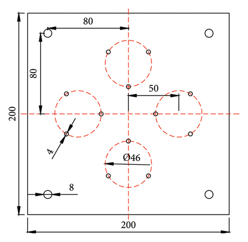
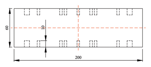
2.1.2. Rupture Damage Creation
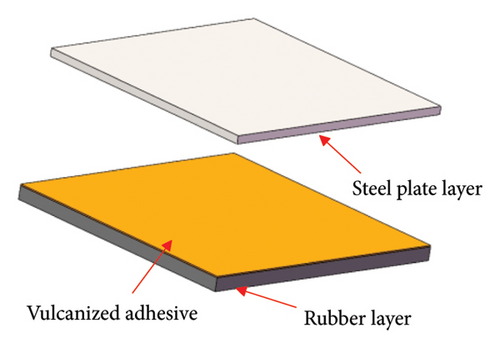
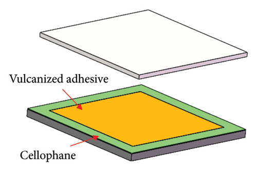
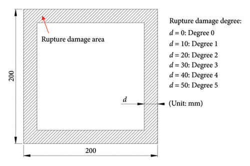
Due to the inability to obtain bearings with multiple damage degrees using the compression-shear testing machine, and the operational difficulties and uncontrollable damage degrees encountered when using cutting tools, this study creates rupture damage by separating the rubber and steel plate layers with cellophane, as shown in Figure 6. During the production process of laminated rubber bearing, a vulcanizing adhesive is applied to the overlapping areas of the steel plate and rubber layers. The vulcanized adhesive undergoes a chemical reaction at high temperatures, thereby firmly bonding the rubber and steel plate layers together. In this study, a strip of cellophane was placed around the outer edge of the contact area between the central steel plate and the rubber layer, without using the vulcanizing adhesive (as shown in Figure 6(d)). As a result, in the areas with cellophane, the rubber and steel plates are separated. Depending on the width of the outer area, the bearing’s rupture damage degrees are classified as Degree 0 (0 mm), Degree 1 (10 mm), Degree 2 (20 mm), Degree 3 (30 mm), Degree 4 (40 mm), and Degree 5 (50 mm), as shown in Figure 6(e). Degree 0 signifies that the bearing has no rupture damage (i.e., the bearing is healthy). Two bearings were fabricated for each rupture damage degree, resulting in a total of 12 laminated rubber bearings.
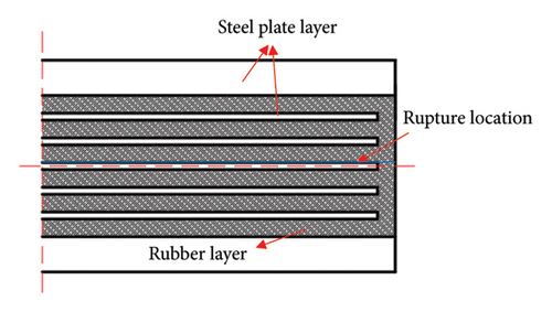
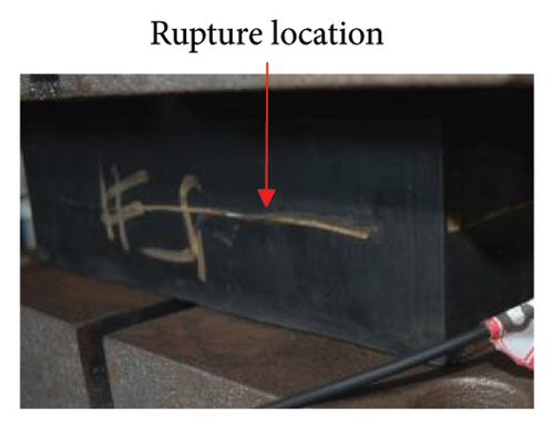
It is worth noting that there are certain differences between the rupture damage of the laminated rubber bearings designed in this study and actual conditions. Therefore, in future research, in addition to developing methods with higher detection accuracy, it will be necessary to obtain detection signals from bearings that more closely resemble or even match actual rupture damage conditions to improve the generalization capability of the prediction model.
2.2. Experimental Scheme
2.2.1. Detection Process
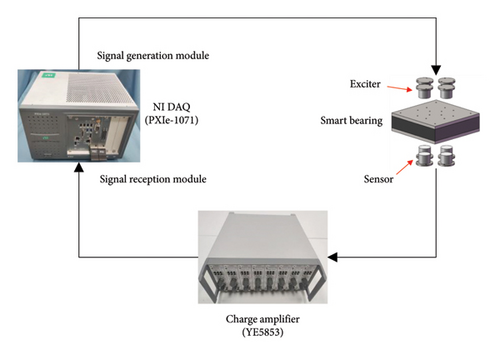
During the detection process, one excitation and one reception strategy are employed. When an exciter is activated, the sensor on the same vertical axis collects the vibration signal.
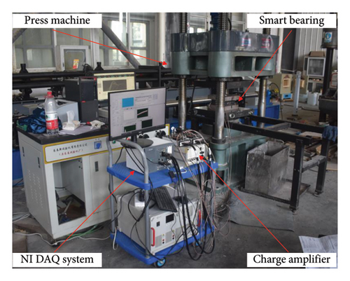
The general process for detecting rupture damage in laminated rubber bearings based on the active sensing method is shown in Figure 7. The detecting system mainly consists of the NI DAQ system (NI PXIe-1071), piezoelectric transducers, and charge amplifier (YE5853). The NI DAQ system serves a dual purpose of generating excitation signals and acquiring detection signals. In this study, the excitation signal was a swept frequency signal with a duration of 1 s, an amplitude of ±10 V, and a frequency range of 1–100 kHz. In addition, the sampling frequency was 1 MHz, and the acquisition time was 1.5 s, starting 0.2 s early to fully capture the vibration signal. The exciter converts the excitation signal into a vibration signal, while the sensor converts the received vibration signal, which penetrates the entire laminated rubber bearing, into a charge signal. The charge amplifier converts the charge signal into a voltage signal and amplifies it simultaneously. In this study, the charge amplifier had a gain of 30, a sensitivity of 2.4, and allowed signals with frequencies below 100 kHz to pass through.
2.2.2. Loading Scheme
To obtain detection signals from the bearings under different axial pressures and improve the model’s applicability, this study designed the loading scheme shown in Figure 8. As illustrated in Figure 8, a total of 10 levels of axial pressure (i.e., 0, 1, 2.5, 5, 7.5, 10, 12.5, 15, 17.5, and 20 MPa) were designed. Once the axial pressure stabilized, the active sensing method testing was conducted. Among them, the setting of 1 MPa is used to simulate a scenario where there is an axial force acting on the bearing, but its magnitude can be almost negligible. In this experiment, a microcomputer-controlled electrohydraulic servo compression–shear testing machine was used to apply pressure to the laminated rubber bearing, with a maximum loading pressure of up to 2000 kN (as shown in Figure 9). The loading scheme was carried out three times in total. Before each loading, the transducers needed to be reinstalled to ensure that the proposed machine learning model takes into account the impact of installation errors on the detection signals.
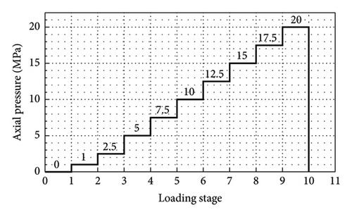
According to the Chinese code standard for seismic isolation design of the building (GB/T 51408-2021) [16], for standard fortified buildings, the maximum design axial pressure of laminated rubber bearings under gravity loads and rare earthquakes are 15 and 30 MPa, respectively. In addition, the axial pressure limit of the bearings used in this study is not less than 90 MPa. Therefore, it is reasonable to set the maximum axial pressure loading value at 20 MPa. This ensures that the bearings will not experience cumulative damage during the experiment and covers the axial pressure values encountered by most bearings in use. Given that the excitation of the exciters and the collection of detection signals require a certain amount of time, it is necessary to uphold the stability of axial pressure during this duration.
3. Experimental Results
Through experiments, 240 detection signals were collected from two laminated rubber bearings with the same degree of rupture damage, resulting in a total of 1440 datasets.
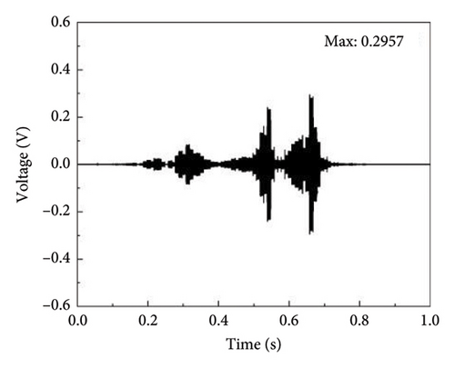
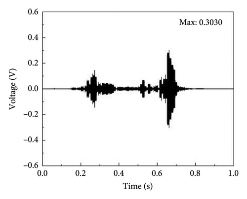
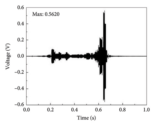
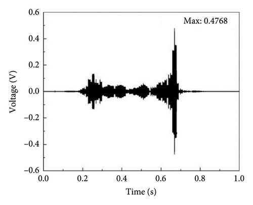
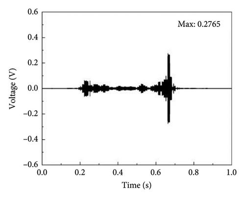
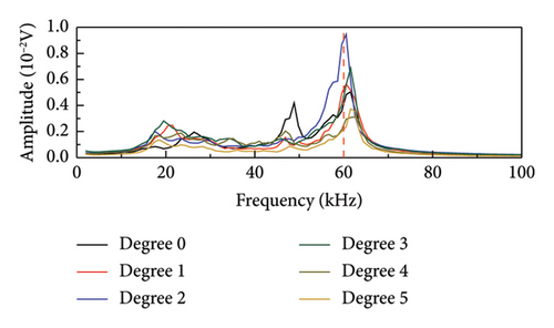
The time histories and frequency spectra of the detection signal for bearings under zero axial pressure and different degrees of rupture damage are shown in Figures 10 and 11, respectively. As shown in Figure 10, the waveforms of the detection signals in the time histories exhibit certain similarities under different degrees of damage, but the variations in the maximum amplitude do not follow a clear pattern. Figure 11 shows that the frequencies corresponding to the maximum amplitude in the frequency domain plots of the detection signals for bearings under different degrees of damage are close, all falling within the range of 60–65 kHz.

WPD was applied to the detection signals under these conditions, as illustrated in Figure 12. For this analysis, an 8-layer Daubechies5 (“db5”) wavelet packet base is utilized, giving rise to a range of i values extending from 1 to 256. Since the wavelet coefficients are mainly concentrated in the first 64 frequency bands, only the wavelet coefficients of the first 64 frequency bands are plotted for convenience. As seen in Figure 12, there are differences in the wavelet packet energy spectra under different degrees of damage, but no clear pattern is observed.
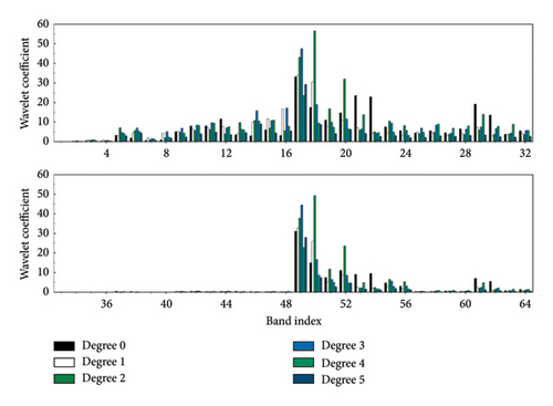
As shown in Figures 10, 11, and 12, the degree of rupture damage has a significant impact on the time history, frequency spectrum, and wavelet packet energy spectrum of the detection signals. However, directly determining the damage degree of the bearings based on the time history, frequency spectrum, and wavelet packet energy spectrum of the detection signals is challenging. Therefore, it is necessary to use machine learning techniques to establish the relationship between the detection signal and the degree of rupture damage.
4. Rupture Damage Detection Method Based on the 1DCNN–LSTM–BO–XGB Algorithm
This section first presents the flowchart of the rupture damage detection method proposed in this paper. Following that, the modeling process of the 1DCNN–LSTM–BO–XGB algorithm is described in detail.
4.1. Rupture Damage Detection Method
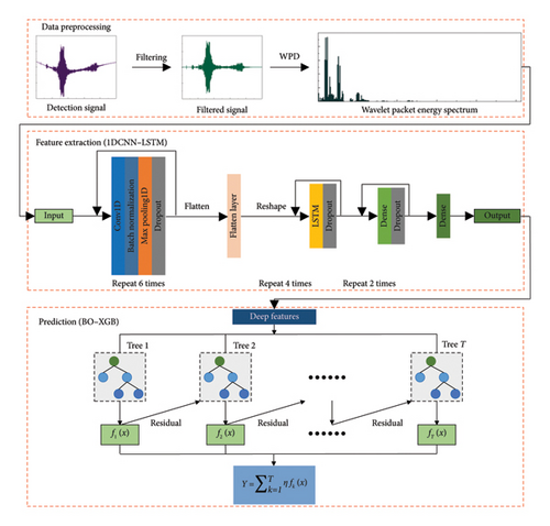
The process for detecting the degree of rupture damage in laminated rubber bearings based on the active sensing method and the 1DCNN–LSTM–BO–XGB algorithm is shown in Figure 13. First, the detection signals of the bearing are obtained using the active sensing method, followed by preprocessing and WPD to obtain the wavelet packet energy spectra. Then, the wavelet packet energy spectra are imported into the 1DCNN–LSTM model for deep feature extraction, and the extracted features are used as input parameters for the BO–XGB model to predict the rupture damage degree of the bearing.
4.2. 1DCNN–LSTM–BO–XGB Algorithm
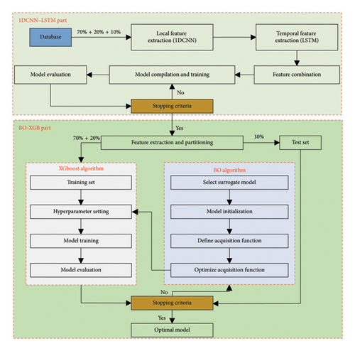
The proposed 1DCNN–LSTM–BO–XGB algorithm in this study is mainly divided into two parts: the 1DCNN–LSTM part and the BO–XGB part. The 1DCNN-LSTM part is used to extract deep features from the wavelet packet energy spectra of the detection signals, while the BO–XGB part is used to establish a high-accuracy prediction model for rupture damage degree. The specific implementation steps are illustrated in Figure 14.
4.2.1. 1DCNN–LSTM Part
1DCNN is a variant of CNNs specifically designed for processing one-dimensional data, such as time series, signal processing, and sequential data. It offers advantages such as local feature learning, parameter sharing, translation invariance, and high computational efficiency [17, 18]. Unlike two-dimensional CNNs, which handle 2D images, 1DCNN slide convolutional kernels over a one-dimensional space, capturing local patterns in the data and effectively extracting features while maintaining computational efficiency [19].
The LSTM algorithm is a special form of RNN specifically designed for processing and predicting time series data [11]. Traditional RNNs, with their inherent recurrent structure, can capture temporal dependencies in sequential data. However, they often face issues such as vanishing or exploding gradients when dealing with long sequences, making it difficult for the network to remember long-term dependencies. LSTM addresses this problem by introducing a specially designed unit structure, the LSTM cell, which enables the network to better capture and retain long-term dependencies.
Therefore, this study utilizes a 1DCNN to extract local high-level features from the wavelet packet energy spectra of detection signals, and an LSTM to further extract their temporal features. The 1DCNN–LSTM part mainly consists of a database, 1DCNN layers, LSTM layers, and fully connected layers. First, the detection signals received by the sensors undergo filtering and WPD to obtain the wavelet packet energy spectra (i.e., the database in Figure 14). The database is randomly divided into three parts in a 7:2:1 ratio: training, validation, and test sets, which are used for model training, validation, and testing, respectively.
First, local features are extracted through six 1DCNN layers, all with a kernel size of 3 and an L2 regularization factor of 0.001. The number of filters in these layers, in sequence, are 128, 256, 512, 1024, 2048, and 4096. Each convolutional layer is followed by a batch normalization layer, a max-pooling layer (with a pool size of 2), and a dropout layer (with a dropout rate of 0.1), which serve to extract the local features, reduce the dimensionality of the data, and enhance the generalization ability of the model, respectively. After extracting local features through the 1DCNN layers, a flatten layer is used to flatten the data, followed by a reshape layer, configured with the parameters (2, 4096), to adjust the data into a shape suitable for input into the LSTM network to further extract temporal features. The LSTM layers consist of four layers, with the number of units in the sequence being 2048, 1024, 512, and 256. All LSTM layers use the ReLU activation function and are followed by dropout layers with a dropout rate of 0.1. Finally, there are three fully connected layers (Dense) with the number of units in the sequence being 512, 256, and 128, each with an L2 regularization factor of 0.001. Each layer is followed by a dropout layer with a dropout rate of 0.1 to further prevent overfitting. The model’s output layer is a softmax layer with 6 units, corresponding to the 6 classification labels. In addition, the model’s optimizer is Adam, with an initial learning rate set to 1e − 4. The loss function used is categorical cross-entropy, and the evaluation metric is accuracy. The stopping criterion is when the iteration count reaches the set value (1000).
After multiple iterations of training, the 1DCNN–LSTM model with the best predictive performance is saved, and the output (one-dimensional vector) from the last fully connected layer (i.e., the layer with 128 units) is extracted as input features for the BO–XGB model.
4.2.2. BO–XGB Part
The BO algorithm is a global optimization method designed for optimizing black-box functions with high computational costs [20]. This approach involves constructing a probabilistic model of the objective function (typically a Gaussian process) and using an acquisition function to intelligently select the next evaluation point, thereby balancing exploration and exploitation to gradually approach the optimal solution. Unlike traditional grid search and random search, the BO algorithm excels in applications such as hyperparameter tuning, where it can find better solutions with fewer iterations. Its primary advantages lie in its efficiency and global optimization capabilities, making it particularly suitable for complex optimization problems with nonanalytic expressions and high computational costs [21, 22].
In 2016, Chen and Guestrin introduced the XGB algorithm based on the traditional gradient boosting trees (GBTs) algorithm [23]. Compared to traditional GBT, the XGB algorithm integrates pioneering techniques and optimization strategies, including the incorporation of regularization terms, parallel computing, Taylor expansion, and approximate algorithms. As a result, XGB demonstrates significant advantages in computational efficiency, overfitting prevention, missing value handling, model flexibility, robustness, interpretability, and early stopping mechanisms. The core idea of the XGB algorithm is to iteratively build new trees to correct the prediction errors of the previous trees, thereby continuously improving the model’s prediction accuracy.
Therefore, based on the deep features extracted from the 1DCNN–LSTM part, this study establishes a high-precision rupture damage degree prediction model using the XGB algorithm. The BO algorithm is employed to optimize the key hyperparameters of the XGB model, aiming to find the global optimal values of the hyperparameters with as few iterations as possible, thereby improving training efficiency and prediction accuracy. The deep features extracted from the 1DCNN–LSTM part are randomly divided into training, validation, and test sets in a 7:2:1 ratio. First, a reasonable search range for the hyperparameters in the XGB model is set based on experience. In this study, the hyperparameters being optimized are the number of trees and the maximum depth of each tree, with search ranges of 100–2000 and 1–20, respectively. During each iteration of the BO algorithm, the potential performance of new hyperparameter combinations is first predicted using a surrogate model, specifically Gaussian process regression (GPR), based on the existing hyperparameter combinations and their corresponding performance. The BO algorithm then optimizes the acquisition function, specifically expected improvement (EI), based on these predictions to select a new hyperparameter combination, which is subsequently used to train the XGB model. After training, the XGB model is evaluated on the validation set to record its performance. These performance results are fed back into the BO algorithm, which further updates the surrogate model and reoptimizes the acquisition function to select new hyperparameter combinations, repeating the process. This process continues until a predefined stopping criterion is met. In this study, the stopping criteria are when the iteration count of the BO algorithm reaches 200. After 200 iterations, the model with the highest test set accuracy, where the difference in accuracy between the training and test sets is within 0.05, is selected as the final model.
It is important to note that the parameter values in the above algorithm were determined through a trial-and-error strategy. When addressing different problems, these parameters may need to be adjusted based on the model’s prediction results.
4.3. Limitations of the Proposed Method
In the rupture damage detection method proposed in this study, the most important component is the prediction model. In this method, the limitations of the model are the limitations of the method itself. For prediction model constructed based on data-driven approaches, their limitations usually stem from the database used. Due to restrictions in the types and ranges of parameters in the database, such as damage occurring only at specific locations of the bearing, the proposed method is not yet fully applicable to all possible damage locations and degrees.
To reduce the limitations of the proposed method, additional experiments and simulations can be conducted to obtain detection signals under conditions of different damage locations and varying degrees of damage, further enriching the database. This will expand the scope of the database and improve the model’s generalization ability, ultimately making it applicable to damage at any location and of any degree within the bearing.
Furthermore, in addition to rupture damage, bearings may also face other types of damage, such as aging damage. In future research, it is necessary to further consider the coupling effects between multiple types of damage.
5. Detection Results of Rupture Damage
5.1. Evaluation Indicators
5.2. Prediction Results of the Proposed Model
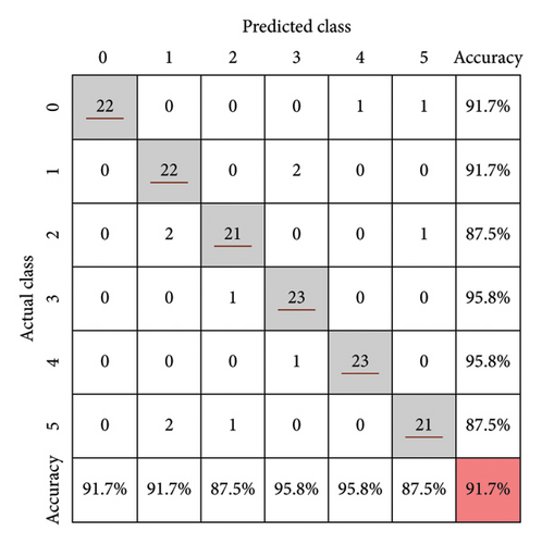
After multiple iterations of training, the optimal 1DCNN–LSTM model achieved accuracy values of 99.9%, 90.0%, and 91.7% on the training, validation, and test sets, respectively (as shown in Figure 15). It can be observed that the model’s predictive performance on the training set is slightly better than on the test set, with a difference in accuracy of 8.2% (or in other words, the accuracy on the training set is 8.9% higher than on the test set).
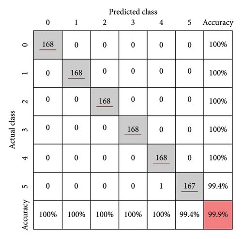
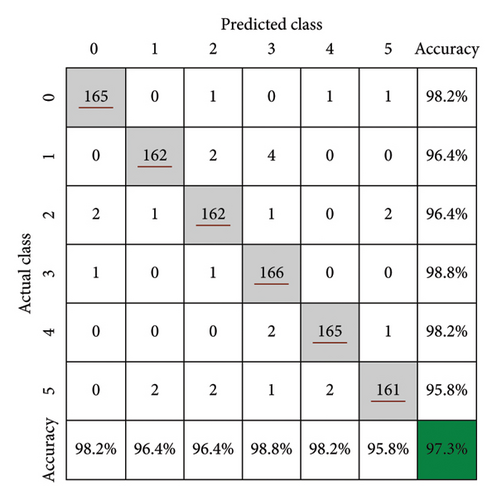
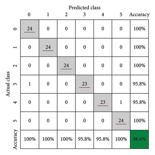
The 1DCNN–LSTM model was used to perform deep feature extraction on the wavelet packet energy spectra of 1440 samples, which were then used as input parameters for the BO–XGB model. After multiple iterations, the optimal hyperparameter combination was found to be as follows: the number of trees was 1700 and the maximum depth of the trees was 15. The prediction results of the 1DCNN–LSTM–BO–XGB model established in this study on the training and test sets are shown in Figure 16. The model achieved an accuracy of 97.3% on the training set, with recognition accuracy for different damage degrees of 98.2% (Degree 0), 96.4% (Degree 1), 96.4% (Degree 2), 98.8% (Degree 3), 98.2% (Degree 4), and 95.8% (Degree 5), respectively. On the test set, the model achieved an accuracy of 98.6%, with recognition accuracy for different damage levels of 100% (Degree 0), 100% (Degree 1), 100% (Degree 2), 95.8% (Degree 3), 95.8% (Degree 4), and 100% (Degree 5), respectively. Compared to the 1DCNN–LSTM model, the test set accuracy increased by 6.9%, reaching 98.6%. In addition, the difference between the training and test sets’ accuracy was only 1.3%, which is significantly lower than the 8.2% difference observed in the 1DCNN–LSTM model (an improvement of 84.1%). The excellent performance of the model indicates that the proposed hybrid algorithm is capable of deeply extracting features from the wavelet packet energy spectra and provides a more accurate model for predicting rupture damage degrees. The study also demonstrates that combining the active sensing method with a machine learning algorithm is highly feasible for accurately detecting the damage degree of laminated rubber bearings.
5.3. Comparison With Other Algorithms
To further demonstrate the superiority of the proposed algorithm in establishing the rupture damage detection model, this study conducted a comparative analysis between the proposed model and several models based on single algorithms. The results are shown in Table 2. It can be observed that although the proposed model does not achieve the same level of prediction accuracy on the training set as the 1DCNN model and the XGB model (both of which reached 100% accuracy), it significantly outperforms other algorithms on the test set. Moreover, the proposed model exhibits no overfitting, or the degree of overfitting is very low, whereas other models show varying degrees of overfitting. Therefore, the proposed algorithm has promising potential for application in rupture damage detection.
| Models | Accuracy | ||
|---|---|---|---|
| Training set (%) | Validation set (%) | Test set (%) | |
| 1DCNN-LSTM-BO-XGB | 97.3 | 97.2 | 98.6 |
| 1DCNN-LSTM | 99.9 | 90.0 | 91.7 |
| 1DCNN | 99.9 | 87.5 | 88.9 |
| LSTM | 18.9 | 20.8 | 25.0 |
| XGB | 100 | 86.5 | 90.3 |
| SVM | 83.1 | 68.1 | 66.7 |
The differences in accuracy among the methods are primarily due to their architectural characteristics and capabilities in handling data. The 1DCNN–LSTM–BO–XGB method achieves superior accuracy by combining 1DCNN, LSTM, BO, and XGB, enabling it to effectively capture local features, temporal dependencies, and nonlinear relationships, while BO optimizes hyperparameters. In contrast, standalone 1DCNN and LSTM methods are limited in capturing complex global relationships. Similarly, although XGB and SVM methods perform well in specific scenarios, they are generally less effective than deep learning methods for capturing intricate local features and temporal dependencies.
6. Conclusions
- 1.
Multiple bearings with controllable rupture damage degrees were fabricated by using cellophane to separate the rubber and steel plate layers. Based on the active sensing method, a database containing 1440 samples was collected and established.
- 2.
The method of further feature extraction using the 1DCNN–LSTM algorithm and using these features as input parameters for the BO–XGB algorithm significantly improves the accuracy of rupture damage detection. Compared to traditional single algorithms, this hybrid approach better captures and utilizes complex features in the signals. The proposed 1DCNN–LSTM–BO–XGB model achieved accuracy values of 97.3%, 97.2% and 98.6% on the training and test sets, respectively, significantly outperforming other algorithms such as 1DCNN–LSTM (99.9%, 90.0%, and 91.7%), 1DCNN (99.9%, 87.5%, and 88.9%), LSTM (18.9%, 20.8%, and 25.0%), XGB (100%, 86.5%, and 90.3%), and SVM (83.1%, 68.1%, and 66.7%).
- 3.
To expand the application scope of the proposed method, future research should enrich the database by including a wider range of parameters through experiments and simulations, such as damage types, locations, and degrees.
Conflicts of Interest
The authors declare no conflicts of interest.
Funding
This research was supported by the National Natural Science Foundation of China (Grant no. 52308322), the Sichuan Province Innovative Talent Funding Project for Postdoctoral Fellows (Grant no. BX202314), and the Fundamental Research Funds for the Central University.
Open Research
Data Availability Statement
The data that support the findings of this study are available from the corresponding author, Yi Zeng, upon reasonable request.


