Mesoscale models are crucial for the refined analysis of material damage behaviors. However, it remains a challenging task to calibrate a mesoscale model so as to accurately simulate the mechanical behaviors (MBs) of macroscale structural components. The models may be nonlinear, involve numerous material parameters (MPs), and be large-scale. In addition, solutions to inverse problems may lack accuracy or be nonunique. A recent emerging method, physics-informed neural network (PINN), combines deep learning with physical laws to solve complex problems and significantly reduce computational costs. This paper presents an effective PINN approach for mesoscale model calibration. The approach establishes a relationship between the MPs of a mesoscale model and the MBs of structural components using PINN, with constraints based on known physical relationships. Both forward PINN (MPs as inputs and MBs as outputs) and reverse PINN (swapping inputs and outputs) models are used. Calibration is achieved efficiently by combining the forward PINN model with an optimization algorithm or directly using the reverse PINN model. Validation is performed using a mesoscale concrete model in peridynamics (PDs). The relationship between the elastic modulus of bonds in PD and MBs of components is constrained by physical laws. The datasets are generated through OpenSees analysis. The PINN method demonstrates its effectiveness, particularly with the reverse model, which is both efficient and accurate.

1. Introduction

Mesoscale models are designed to accurately capture the microscopic damage mechanisms within materials. However, when employing mesoscale models to simulate structural components, calibration of the material parameters (MPs) is required. This process is often elaborate and time-consuming, primarily due to the typically extensive computational scale, encompassing nonlinearities and numerous parameters for adjustment. In recent years, the rapid advancement of computer technology has propelled the progress of machine learning (ML). In this evolving technological landscape, ML has emerged as a powerful tool for modeling and solving complex engineering problems [1]. MLs have demonstrated remarkable success in fitting structural responses with high precision and efficiency [2–5]. By leveraging well-constructed neural network models, the process of fitting structural responses becomes not only rapid but also remarkably accurate, leading to a substantial reduction in the computational time traditionally required for such tasks. Many scholars have applied ML to capture the complex nonlinear plastic behavior of materials or structures. For example, Siow et al. employed ML to extract the main structural damage-sensitive feature while maintaining dynamic characteristics [6]. Fu and Wei proposed a two-stage ML–based method to model the elastic modulus of concrete [7]. Teng et al. employed a convolutional neural network (CNN) to extract damage features of the bridge population [8]. Although ML has made significant advancements, the calibration process for mesoscale model parameters is notably complex. Traditional ML methods may struggle to meet some physical requirements. Recently, a kind of ML method called physics-informed neural network (PINN) has been proposed, which integrates physical laws into the architecture of neural networks, offering a unique blend of traditional numeric simulation and ML [9]. This integration enables PINN not only to learn from data but also to respect the governing physical principles, ensuring more reliable predictions. Currently, numerous scholars have also employed PINN to study the nonlinear behavior in civil structures. Jeong et al. proposed a PINN–based topology optimization, which opened up a new avenue for structural design [10]. Pu et al. proposed a PINN model to enhance the fitting of nonlinear data with prior knowledge, providing greater stability and accuracy than traditional DNNs, especially in noisy conditions and with inadequate samples [11]. Yamaguchi and Mizutani proposed a PINN–based damage identification algorithm to assess earthquake-induced damages in reinforced concrete bridge piers, achieving precise parameter estimations [12].

The advent of PINN represents a significant advancement in the ability to integrate data-driven insights with physical laws. This integration can be crucial in the field of fracture and damage simulation. Within this domain, various models have been developed, including the discrete cohesive crack model, phase field model, nonlocal damage model, and peridynamics (PDs). The discrete cohesive crack model offers precise control over crack initiation and propagation but requires preinserted cohesive elements and crack-tracking strategies, limiting its wider applicability [13]. The phase field model effectively handles complex crack patterns with simple implementation but incurs high computational costs due to its implicit numerical methods [14]. The nonlocal damage model provides mesh-independent solutions, yet it may suffer from spurious damage growth across overly extensive areas due to constant interaction domains [15]. In contrast, PD is a nonlocal continuum theory developed by Silling and Lehoucq [16, 17]. Due to the absence of spatial derivatives in its governing equations, PD excels in addressing discontinuous field problems, such as cracking and fracture [18–22]. PD theory can be categorized into bond-based PD (BPD) and state-based PD (SPD). In BPD, it is assumed that points within the horizon are interconnected by fictitious bonds. The force exerted by each bond is assumed to be along with the bond itself, and the magnitude can be determined based on the bond’s elongation and a suitable uniaxial material’s constitutive model. Due to its simplicity and practicality, BPD has been extensively applied to the refined simulation of various damage and fracture problems. For example, Huang, Zhang, and Qiao proposed a refined BPD to simulate damage and progressive failure of concrete materials and structures under various loading [23]. Li and Guo proposed a mesoscopic BPD model for mesofracture simulation of the cracking process in concrete, i.e., truss elements with appropriate stiffness properties are used to represent the PD bonds [24]. Zhang et al. proposed a novel coupled axial–shear interaction bond-slip BPD model to simulate the relative slip and interface damages between the concrete and steel [25]. Despite the widespread application of BPD to numerous engineering problems, the practical implementation often requires elaborate calibration, particularly for nonlinear materials. In addition, the MPs will vary with changes in the PD model’s grid spacing dx. This inefficiency in calibration complicates the use of PD and restricts its practical application in engineering to some extent.

This paper utilizes PD as a case study to demonstrate how the PINN model can delineate the relationship between MPs and mechanical behaviors (MBs). In this context, “mesoscale” specifically refers to a refined PD model designed to target damage processes at the millimeter scale or smaller. This definition contrasts with the conventional interpretation of mesoscale, which typically pertains to phases such as aggregates and mortar [15]. Specifically, the paper develops the PINN by incorporating the mesoscale elastic modulus formula from PD theory into the loss function of a CNN model. Initially, a forward PINN model is developed where MPs serve as inputs (“causes”) and MBs as outputs (“effects”). Then, an optimization process is used to align the predicted MBs with the targeted values by iteratively adjusting the MPs. Lastly, a “reverse” PINN model is designed, where MBs are the inputs and MPs are the outputs, effectively flipping the relationship from outcomes back to causes. This approach streamlines the calibration process, eliminating the need for mathematically solving the inverse problem and demonstrating the capability to rapidly and accurately complete the calibration of parameters. The approach proposed in this paper offers the following advantages: (1) An efficient PINN model is developed to calibrate mesoscale models using ML with integrated physical constraints. (2) Both forward and reverse PINN models are comparatively explored for calibrations, with forward models combined with optimization techniques. (3) Relationships are established between the MBs of macroscale concrete structural components and the MPs of mesoscale PD bond models. (4) The training datasets are analyzed using the nonlinear finite element software, OpenSees, which utilizes its comprehensive material libraries, nonlinear algorithms, and parallel computing capabilities.

2. The PINN Model

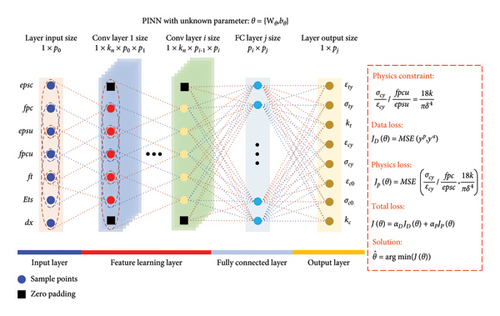
The proposed PINN model is constructed by the input layer, convolution layer, fully connected (FC) layer, and output layer. Taking the forward PINN model as an example, Figure 1 illustrates the workflow of the entire PINN, detailing the process when the inputs are MPs with dx and the outputs are MBs. Further details about MPs and MBs will be introduced in the next section. In Figure 1, p_i denotes the output size of the ith layer, θ represents the model parameters, k_n represents the kernel size of the convolution layer, and MSE represents the mean square error function.

Details are in the caption following the image — **Figure 1**
Open in figure viewer PowerPoint

Illustration of the proposed physics-constrained neural network.

2.1. Convolution Layer, Pooling Layer, and FC Layer

The convolution layer is a part of the CNN architecture, which can significantly reduce the number of parameters and enhance feature detection by preserving the relational properties of the data. A convolutional layer’s dimensions are characterized by its height (in the case of 1D convolution, height = 1), width, depth, and the number of filters (output channels). Each layer consists of a set of learnable kernels (also known as filters) typically sized at 1 × k_n. Notably, in order to ensure that the length of the output is equal to that of input in the temporal space, zero-padding is added at the input. The number of zero-padding P can be calculated by P = k_n − 1. The dimension of layer output y^(l) can be different from the layer input x^(l). Thereby, the output of the j th output channel

can be obtained as

()

where the symbol ″∗” denotes the 1D convolution operator, superscript l is the layer index, subscript i is the i th input channel, W is the receptive field, and b is the bias vector added to the summed term. Subsequently, it is essential to incorporate a nonlinear activation function following the convolutional layer to facilitate easier learning. The activation layer introduces nonlinearity to the model and the entire network without altering the receptive field of the convolutional layer. This paper employed the rectified linear unit (ReLU) [26] as the nonlinear activation function, which can be described as

()

In the CNN model, pooling layers are typically employed to reduce the spatial size of feature maps while dealing with large input data. Generally, pooling methods include max pooling and average pooling, which extract the maximum or average values from the pooling window, respectively. However, pooling layers compress feature maps, which can lead to loss of critical information, reduced precision in tasks needing high accuracy, and obscured fine details [27]. In the proposed PINN model, the use of pooling layers would result in shorter output lengths, which is undesirable for the regression problems between MBs and MPs. Therefore, the application of pooling layers is restricted in the proposed PINN architecture.

FC layers are typically employed in the latter stages of CNNs to facilitate the transition from feature extraction to output generation. Each neuron in a FC layer is interconnected with all activations from the previous layer, effectively integrating learned features by computing a weighted sum over them, followed by adding a bias term (as shown in Figure 2).

2.2. Loss Function and Solution

As shown in Figure 1, the total loss function J(θ) is divided into two forms, i.e., the data loss J_D(θ) and physics loss J_P(θ), which can be calculated as

()

where θ represents the model parameters and α_D and α_P are the weights of data loss and physics loss, respectively. In this paper, we specify α_D and α_P as 0.9 and 0.1, respectively. J_D(θ) and J_P(θ) can be obtained by

()

where y^p and y^a denote the predicted and actual outputs, respectively. k is the bulk modulus of the material and δ is the horizon size. σ_cy and ε_cy are the MBs, while fpcu and epsu are the MPs, and these parameters will be illustrated in detail in the next section. Equation (5) can be obtained from the PD theory and will be elaborated upon in the following section. Therefore,

will be updated based on the optimization function as

()

It is important to note that the step size for updating parameters in neural networks is determined by the gradient. Taking the forward PINN model as an example, we denote the two output variables ε_cy and σ_cy as Y₁ and Y₂, respectively, and the two input variables epsc and fpc as X₁ and X₂, respectively. Then, equation (5) can be rewritten as

()

According to the chain rule, the partial derivative of the loss function with respect to θ can be expressed as

()

where ∂Y₁/∂θ and ∂Y₂/∂θ are obtained directly by automatic differentiation employed in state-of-the-art DL frameworks. Furthermore, ∂J_p(θ)/∂Y₁ and ∂J_p(θ)/∂Y₂ can be calculated as

()

3. Mesoscale Simulation of Concrete Using a Fine BPD Model

As shown in Figure 3, X represents a PD point, H_X represents the horizon of point X, and δ is the radius of the horizon. For any PD point X^′ within the horizon, ξ and y are the relative position vectors between X and X^′ in the initial configuration and the current configuration, respectively. η represents the relative deformation of X and X^′, i.e., ξ = X^′ − X, η = u(X^′) − u(X), y = η + ξ, where u(X) and u(X^′) are the displacement vector of X and X^′, respectively. In BPD theory, point X is assumed to be connected with other PD points within its horizon by bonds, and f(X, X^′) denotes the force of each bond acted on point X. Therefore, the motion equation of BPD can be written as

()

where ρ denotes density,

is the acceleration vector of point X, V_ξ denotes the volume of a sphere with X as the center and ‖ξ‖ as the radius, and b(X) represents the body force. In BPD, f(X, X^′) can also be written as f(ξ, η). f(ξ, η) and f(−ξ, −η) represent a pair of bond forces that are equal in magnitude, opposite in direction, and parallel to the relative position vector in the current configuration. f(ξ, η) can be calculated as

()

where n = η + ξ/‖η + ξ‖ denotes the direction of the bond in deformation configuration and s denotes the stretch of the bond, i.e.,

()

According to the micropotential principle [28], the total strain energy of point X in isotropic elastic materials can be obtained as

()

where w(ξ, η) denotes the energy of each bond and c₀ represents the microscopic elastic modulus in BPD. This is required to be equal to strain energy density in the classical theory, i.e.,

()

where k denotes the bulk modulus of the material. Based on equations (13) and (14), c₀ can be obtained as

()

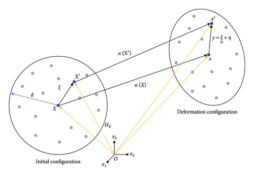
Therefore, in the elastic state, the microelastic modulus in BPD can be determined through analytical derivation. However, when the material exhibits nonlinear behavior, which is particularly evident in simulations of reinforced concrete components characterized by strong nonlinearity, the microelastic modulus may no longer fully comply with equation (15), and other nonlinear MPs become difficult to estimate. These parameters can only be inferred through postcalculation analysis, leading to a significant expenditure of time in the iterative calibration of these parameters when simulating reinforced concrete components with BPD. This scenario highlights the intricacies involved in modeling such materials and the challenges associated with accurately predicting the response. The following will introduce the parameters that need to be calibrated when simulating concrete materials using the fine BPD model.

3.1. The MPs of the BPD Concrete Model

In simulations utilizing BPD, the linear tension softening model in OpenSees (i.e., Concrete02 Material [29]) is chosen for the concrete bond model. As shown in Figure 4, this model can adeptly simulate the complex strong nonlinear behavior of concrete under compression or tension with a limited set of parameters, where epsc and fpc represent the yield compressive stain and stress of concrete, respectively. epsu and fpcu denote the ultimate compressive strain and stress. λ is the ratio between the unloading slope (at ultimate strain) and the initial slope. ft is the yield tensile stress, Ets is tension softening stiffness, and E₀ is initial stiffness which can be calculated as E₀ = 2fpc/epsc.

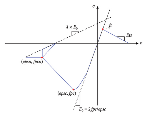
Therefore, in the practical application of this material model for simulating concrete, a total of seven parameters require calibration. This paper primarily focuses on the stress–strain curve of concrete specimens under compression or tension. Considering that parameter λ mentioned previously manifests during the unloading phase, it does not need to be calibrated in this context. Consequently, within the scope of this study, there are six parameters that require calibration in the employed linear tension softening model (refer to Table 1).

Table 1. The parameters that required calibration in the linear tension softening model.

Parameter	Symbol
Yield compressive strain	epsc
Yield compressive stress	fpc
Ultimate compressive strain	epsu
Ultimate compressive stress	fpcu
Yield tensile stress	ft
Tension softening stiffness	Ets

To obtain appropriate BPD model parameters, calibration is typically based on the mechanical properties of standard specimens, with the most commonly used being the tensile and compressive stress–strain curves. This will be detailed in Section 3.2.

3.2. MB of the Concrete Specimen

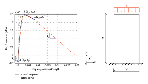
Figure 5 displays the stress–strain curve obtained from the uniaxial tension and compression numerical simulation of standard concrete specimens using the Concrete02 Material in BPD. Through the comprehensive analysis and synthesis of a vast amount of data, this paper identifies eight key data points within the curve to depict the stress–strain behavior of the components as accurately as possible. These key data points include peak points, significant turning points, and the slopes of the descending segments of the curve, which are crucial for defining the mechanical response accurately. It is also noteworthy that the yellow points D and E shown in the Figure 5 are not directly extracted from the curve but are interpolated auxiliary inflection points derived from point B. The specific method used is x_D = (1/2)x_B, y_D = (3/4)y_B, x_E = (1/2)x_B + (1/2)x_D, and y_E = (3/4)y_B + (1/4)y_D. After determining these key points, they are connected with multisegment lines to fit the entire stress–strain curve, as illustrated in Figure 5, where the solid black line represents the stress–strain curve obtained from numerical simulation, and the red dotted line is the fitted curve based on key points. The authors, after validating across all datasets, have found that the selection of these key points can adequately simulate the complete uniaxial tension-compression curve. In the practical application of BPD simulation for concrete, it is common to compare this curve to further simulate the overall hysteretic behavior. Among these eight key points, three are related to tensile behavior: the yield tensile strain ε_ty, yield tensile stress σ_ty, and the slope of the tensile softening segment k_t. The remaining five are related to compressive behavior, including yield compressive strain ε_cy, yield compressive stress σ_cy, strain ε_c0, and stress σ_c0 at the inflection point of the softening segment, and the slope of the compressive softening segment k_c. With these eight data points (see Table 2), it is possible to accurately reconstruct the overall curve.

Table 2. The key data points in the stress–strain curve of the specimen.

Parameter	Symbol
Yield tensile strain	ε_ty
Yield tensile stress	σ_ty
The slope of the tensile softening segment	k_t
Yield compressive strain	ε_cy
Yield compressive stress	σ_cy
Strain at the inflection point	ε_c0
Stress at the inflection point	σ_c0
The slope of the compressive softening segment	k_c

4. Calibration Based on Forward and Reverse PINN Models

This paper utilizes forward and reverse PINN models to predict the relationship between MPs of BPD and MBs of components. For both the two PINN models, a total of 1044 simulation cases were conducted, with 730 cases (70%) used to train the neural network model, 157 cases (15%) used to validate, and the remaining 157 cases (15%) employed to test the accuracy and reliability of the trained model. It is noteworthy that the grid spacing dx needs to be set within BPD simulations. Due to the boundary effects inherent in BPD, if dx is too large, it leads to a reduced number of PD points, thereby accentuating noticeable boundary effects and causing inaccuracies in the simulation. Conversely, if dx is too small, it results in an excessive number of PD points, which does not significantly enhance computational precision but drastically increases computation time. For standard specimens (150mm × 150mm × 300mm), this paper sets dx within the range of 8–20 mm and includes it as one of the input variables for training. Figure 6 illustrates the dimensions and boundary conditions of the PD model of the component, where the model’s width and height are 150 mm and 300 mm, respectively, with a thickness of 150 mm. The PD points at the base of the model are fixed in all three directions, while a uniform displacement is applied to the top in the y-direction to simulate both tensile and compressive conditions.

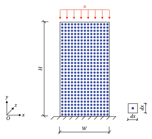
Hence, the forward PINN model predicts MBs based on MPs, and there are seven input variables (six MPs and dx), resulting in eight output variables (eight key data points). Conversely, the reverse PINN model predicts the required MPs based on MBs, and nine input variables are needed (eight key data points and dx), which lead to the output of six MPs.

4.1. Forward PINN Model

In this study, we first establish a forward PINN model. It begins with a sequence input layer of size 7, followed by two 1D convolutional layers, each equipped with 20 filters of size 3 and “same” padding. These layers are interleaved with ReLU activation functions to introduce nonlinearity. The control parameters of the PINN model included a training target minimum error set to 0.0001, a learning rate of 0.001, a mini-batch size of 8, and a total of 50 training iterations. The Adam optimizer is employed with standard parameters (beta1 = 0.9, beta2 = 0.999, and epsilon = 1e − 8). The “mapminmax” function from MATLAB is employed as the normalization method to preprocess the training data. This function applies the following transformation to each feature in the dataset:

()

where X and X^′ are the original and normalized values of the input feature, respectively. X_min and X_max are the minimum and maximum values of the feature across the dataset, respectively. C_min and C_max are the minimum and maximum values of the target range, such as −1 and 1. The input variables were set to dx and MPs used in BPD, and the output variables were set to key data points of the stress–strain curves of the components (MBs) for training. It is worth noting that within our model parameters, the ratio of fpc to eps is held constant for each dataset, as both are input parameters throughout training.

Figure 7 compared the convergence histories of CNN and FC network (FCNN). It is important to note that these two models used in our comparisons are designed with a comparable number of trainable parameters, ensuring a fair comparison in terms of model capacity. Based on this, it can be observed that CNN demonstrates superior efficiency and effectiveness. The CNN model not only converges faster but also achieves lower loss and L2 norm error across epochs. By the 50th epoch, the loss stabilized at 0.035 and the L2 norm error at 0.073 in the CNN model.

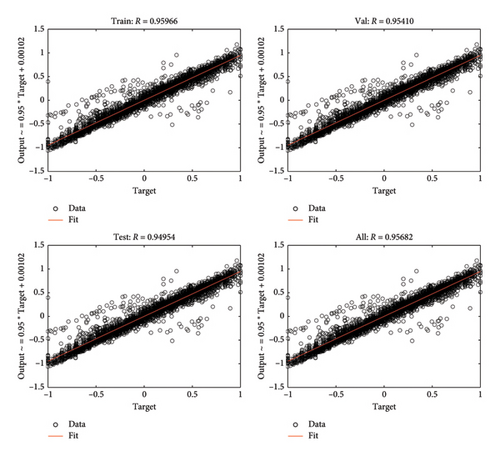
The sample correlation coefficient R is often used to measure the degree of linear correlation between two sets of data. The range of R is from 0 to 1, and a value of 1 shows that the predictions are correct. As depicted in Figure 8, the R values for the training, validation, and test sets were 0.95966, 0.95410, and 0.94954, respectively, all of which are close to 1. This indicates the high accuracy of the trained PINN.

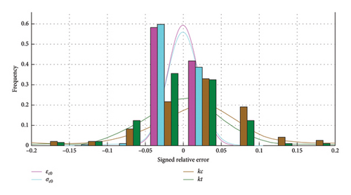
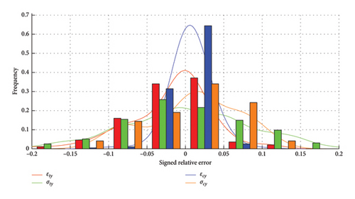
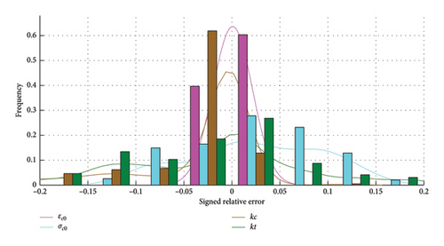
A set of 157 test cases was employed to conduct a more detailed examination of the discrepancies between the predicted values and actual values for each MB. As depicted in Figures 9 and 10, the predicted values of 8 MBs agree well with the expected values. The mean relative error (MRE) calculates the average of absolute errors as a percentage of the real values and is defined as , where and are the real and predicted values, respectively. From the detailed analysis presented in Table 3, it is evident that the proposed forward PINN model can precisely predict three key points of stress and strain in the MBs based on the MPs, with the maximum MRE reaching only 1.70%. While the relative errors for the slopes in the tensile and compressive segments (k_c and k_t) are slightly higher, they remain within acceptable limits at 6.79% and 4.79%, respectively. Notably, the maximum REs across all data points hover around 10%, and the minimum REs are exceptionally low, typically less than 0.01%. These findings robustly confirm the reliability and effectiveness of the trained forward PINN model in capturing the complex dynamics of the simulated materials and behaviors.

Table 3. The REs of the 8 MBs in the forward PINN model.

Parameter	MRE (%)	Maximum RE (%)	Minimum RE (%)
ε_ty	1.70	10.84	0.01
σ_ty	0.87	10.73	0.005
ε_cy	0.93	2.86	0.004
σ_cy	0.95	10.09	0.006
ε_c0	0.20	1.09	0.002
σ_c0	0.60	10.13	0.001
k_c	6.79	13.39	0.005
k_t	4.79	13.77	0.007

After obtaining the trained model, an optimization algorithm will be employed to streamline the traditional calibration process. The initial step involves establishing an optimization challenge with the goal of reducing the discrepancy between the neural network’s predictions (MBs) and the real observed MBs. This is achieved by deploying the global optimization strategy MultiStart in Matrix Laboratory (i.e., MATLAB), which creates numerous initial points within the predetermined parameter value ranges [30]. From these points, a local optimization search commences, employing the capabilities of the fully trained neural network to calculate the outputs (MBs) for a set of given inputs (MPs). In conjunction, a local optimization function LBFGS is utilized to find the global optimum solution. The function aims to minimize the relative error between the MBs calculated by the PINN model and the actual MBs by adjusting MPs, while also incorporating the physical loss J_p(θ) to ensure physical accuracy, i.e.,

()

where i represents the ith MBs, and subscripts p and r denote the predicted and real values, respectively. α_D and α_P are taken as 0.9 and 0.1, respectively.

The accuracy of the optimization algorithm is corroborated by the previous 157 sets of cases. Figures 11 and 12 illustrate that, given specific MBs, the fully trained model successfully determines an appropriate set of MPs through the optimization process. Although a small number of datasets have a maximum RE of about 20%, for the majority of datasets, the error can be controlled within 10%. The outputs generated from these optimization-derived MPs align closely with the initially provided MBs, showing a good level of agreement. The REs for eight parameters are detailed in Table 4. Furthermore, the inputs predicted by the optimization algorithm are compared with the actual MPs, yielding a MRE of 7.47% across six MPs. This indicates the effectiveness of the proposed method in substituting the conventional calibration process, facilitating the swift and precise identification of optimal BPD MPs from essential points on the stress–strain curve.

Table 4. The RE of eight predicted MBs after optimization.

Parameter	MRE (%)	Maximum RE (%)	Minimum RE (%)
ε_ty	3.95	24.39	0.001
σ_ty	6.62	26.07	0.060
ε_cy	1.57	10.05	0.001
σ_cy	4.94	13.03	0.006
ε_c0	0.39	3.06	0.003
σ_c0	6.05	16.29	0.012
k_c	4.42	24.94	0.001
k_t	8.69	25.54	0.001

4.2. Reverse PINN Model

In the reverse PINN model, the layers of the network, division of the datasets, and control parameters remain identical to those of the forward PINN model, with the exception that the input layer size has been adjusted to 8. The distinction lies in the input and output variables: for the reverse PINN model, the input variables are the key data points from the macroscopic stress–strain curve of components (MBs) and the grid spacing dx, while the output variables are the MPs required for use in BPD.

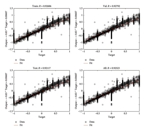
In the reverse PINN model, the R values for the training, validation, and test sets were 0.92606, 0.92792, and 0.92117, respectively (shown in Figure 13). It can be observed that all R values are close to 1, proving the accuracy of the model.

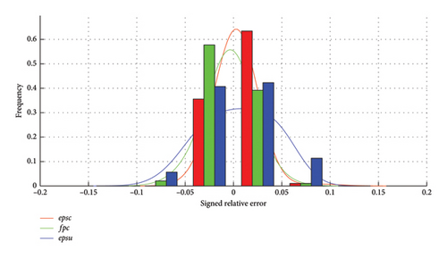
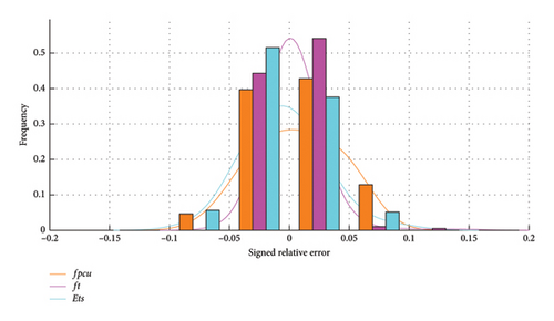
Similar to the forward PINN model, 157 additional test cases are employed to validate the accuracy of the predicted values. Figures 14 and 15 clearly show a good agreement among the six output values. The MRE for the six data points has been listed in Table 5, with the highest relative error being only 3.02%. These results indicate that this methodological approach enables the inverse prediction of essential MPs, facilitating the calibration of fine BPD models for accurate simulation of MBs. This reverse-engineering capability significantly enhances the practical utility of BPD in complex material modeling and structural analysis, demonstrating the versatility and efficacy of integrating ML techniques with traditional computational mechanics methodologies. Table 6 shows that, the forward PINN model combined with an optimization function, required 47.46 s to predict 157 sets of appropriate inputs. In contrast, using the reverse PINN model to predict inputs for the same number of datasets took only 0.68 s. The training times of the forward and reverse models are 43.30 s and 75.10 s, respectively. In contrast, simulating the tension and compression process of the component in OpenSees takes about 2 h. It is obvious that the two proposed PINN models significantly enhance calibration efficiency.

Table 5. The mean relative errors of the six parameters in the reverse PINN model.

Parameter	MRE (%)	Maximum RE (%)	Minimum RE (%)
epsc	0.98	9.81	0.02
fpc	1.44	6.32	0.01
epsu	3.02	8.49	0.07
fpcu	2.92	7.55	0.01
ft	1.01	14.0	0.0001
Ets	2.51	9.80	0.01

Table 6. Comparative analysis of computational costs: forward and inverse PINN vs. OpenSees.

	Training		Prediction (157 sets)		OpenSees (1 set) (h)
	Forward (s)	Reverse (s)	Forward (s)	Reverse (s)	OpenSees (1 set) (h)
Time	43.30	75.10	47.46	0.68	2

It is also worth noting that while the method is efficient and accurate, it has limitations. Specifically, the calibration results are model-dependent, i.e., they may vary and cannot be directly applied across different concrete bond models, which complicates their use in direct engineering applications. Future efforts will focus on expanding mesoscale models, incorporating additional physical constraints and examining complex components such as reinforced concrete to develop practical tools for engineering analyses.

5. Conclusions

This paper presents a PINN approach for effectively calibrating mesoscale models, integrating known physical relationships between MPs and MBs. We established both a forward PINN model, where MPs serve as inputs and MBs as outputs using an optimization algorithm for calibration, and a reverse PINN model, which switches the input and output roles and eliminates the need for optimization. The methods are validated through a mesoscale concrete model using PD, trained and tested on 1044 sets of cases from OpenSees, which offers a well-established framework for structural analysis. The forward PINN model demonstrated high accuracy with a maximum MRE of 6.79% in MBs, while the reverse model further improved efficiency with a maximum relative error of 3.02% in predicting MPs. This study underscores the potential of PINN to streamline and enhance the calibration of mesoscale models, combining accuracy and efficiency, especially notable in the reverse PINN approach. The limit of the method is that calibration results may vary when using different concrete bond models, which can complicate direct engineering applications. Future work will expand on mesoscale models, incorporate more physical constraints, and explore complex components such as reinforced concrete to provide practical tools for engineering analyses.

Conflicts of Interest

The authors declare no conflicts of interest.

Funding

The authors acknowledge the financial support received from the National Natural Science Foundation of China (Grant nos. 52378539 and 51978591).

Acknowledgments

The authors acknowledge the financial support received from the National Natural Science Foundation of China (Grant nos. 52378539 and 51978591).

Open Research

Data Availability Statement

The data that support the findings of this study are available from the corresponding author upon reasonable request.

References

1 Agatonovic-Kustrin S. and Beresford R., Basic Concepts of Artificial Neural Network (ANN) Modeling and Its Application in Pharmaceutical Research, Journal of Pharmaceutical and Biomedical Analysis. (2000) 22, no. 5, 717–727, https://doi.org/10.1016/s0731-7085(99)00272-1, 2-s2.0-0034213103.
10.1016/S0731-7085(99)00272-1
CAS PubMed Web of Science® Google Scholar
2 Thai H.-T., Machine Learning for Structural Engineering: A State-of-the-Art Review, Structures, 2022, Elsevier, Amsterdam, Netherlands.
Google Scholar
3 Liu D., Tang Z., Bao Y., and Li H., Machine-Learning-Based Methods for Output-Only Structural Modal Identification, Structural Control and Health Monitoring. (2021) 28, no. 12, https://doi.org/10.1002/stc.2843.
10.1002/stc.2843
PubMed Google Scholar
4 Bud M. A., Moldovan I., Radu L., Nedelcu M., and Figueiredo E., Reliability of Probabilistic Numerical Data for Training Machine Learning Algorithms to Detect Damage in Bridges, Structural Control and Health Monitoring. (2022) 29, no. 7, https://doi.org/10.1002/stc.2950.
10.1002/stc.2950
PubMed Google Scholar
5 Delgadillo R. M. and Casas J. R., Bridge Damage Detection via Improved Completed Ensemble Empirical Mode Decomposition with Adaptive Noise and Machine Learning Algorithms, Structural Control and Health Monitoring. (2022) 29, no. 8, https://doi.org/10.1002/stc.2966.
10.1002/stc.2966
PubMed Google Scholar
6 Siow P. Y., Ong Z. C., Khoo S. Y., and Lim K.-S., Damage Sensitive PCA-FRF Feature in Unsupervised Machine Learning for Damage Detection of Plate-Like Structures, International Journal of Structural Stability and Dynamics. (2021) 21, no. 02, https://doi.org/10.1142/s0219455421500280.
10.1142/S0219455421500280
Google Scholar
7 Fu B. and Wei X., An Intelligent Analysis Method for Human-Induced Vibration of Concrete Footbridges, International Journal of Structural Stability and Dynamics. (2021) 21, no. 01, https://doi.org/10.1142/s0219455421500139.
10.1142/S0219455421500139
Google Scholar
8 Teng S., Chen X., Chen G., Cheng L., and Bassir D., Structural Damage Detection Based on Convolutional Neural Networks and Population of Bridges, Measurement. (2022) 202, https://doi.org/10.1016/j.measurement.2022.111747.
10.1016/j.measurement.2022.111747
Google Scholar
9 Raissi M., Perdikaris P., and Karniadakis G. E., Physics-Informed Neural Networks: A Deep Learning Framework for Solving Forward and Inverse Problems Involving Nonlinear Partial Differential Equations, Journal of Computational Physics. (2019) 378, 686–707, https://doi.org/10.1016/j.jcp.2018.10.045, 2-s2.0-85057501376.
10.1016/j.jcp.2018.10.045
Web of Science® Google Scholar
10 Jeong H., Bai J., Batuwatta-Gamage C. P., Rathnayaka C., Zhou Y., and Gu Y., A Physics-Informed Neural Network-Based Topology Optimization (PINNTO) Framework for Structural Optimization, Engineering Structures. (2023) 278, https://doi.org/10.1016/j.engstruct.2022.115484.
10.1016/j.engstruct.2022.115484
Google Scholar
11 Pu J., Song W., Wu J., Gou F., Yin X., and Long Y., PINN-Based Method for Predicting Flow Field Distribution of the Tight Reservoir After Fracturing, Geofluids. (2022) 2022, no. 1, 1–10, https://doi.org/10.1155/2022/1781388.
10.1155/2022/1781388
Google Scholar
12 Yamaguchi T. and Mizutani T., A Physics-Informed Neural Network for the Nonlinear Damage Identification in a Reinforced Concrete Bridge Pier Using Seismic Responses, Structural Control and Health Monitoring. (2024) 2024, no. 1, https://doi.org/10.1155/2024/5532909.
10.1155/2024/5532909
Google Scholar
13 Moës N. and Belytschko T., Extended Finite Element Method for Cohesive Crack Growth, Engineering Fracture Mechanics. (2002) 69, no. 7, 813–833, https://doi.org/10.1016/s0013-7944(01)00128-x, 2-s2.0-0037192563.
10.1016/S0013-7944(01)00128-X
Web of Science® Google Scholar
14 Hai L., Wriggers P., Huang Y.-J., Zhang H., and Xu S.-L., Dynamic Fracture Investigation of Concrete by a Rate-Dependent Explicit Phase Field Model Integrating Viscoelasticity and Micro-Viscosity, Computer Methods in Applied Mechanics and Engineering. (2024) 418, https://doi.org/10.1016/j.cma.2023.116540.
10.1016/j.cma.2023.116540
PubMed Google Scholar
15 Huang Y.-J., Zhang H., Zhou J.-J., and Xu S.-L., Efficient Quasi-Brittle Fracture Simulations of Concrete at Mesoscale Using Micro CT Images and a Localizing Gradient Damage Model, Computer Methods in Applied Mechanics and Engineering. (2022) 400, https://doi.org/10.1016/j.cma.2022.115559.
10.1016/j.cma.2022.115559
Google Scholar
16 Silling S. A. and Lehoucq R., Peridynamic Theory of Solid Mechanics, Advances in Applied Mechanics, 2010, Elsevier, Amsterdam, Netherlands, 73–168.
Google Scholar
17 Silling S. A., Epton M., Weckner O., Xu J., and Askari E., Peridynamic States and Constitutive Modeling, Journal of Elasticity. (2007) 88, no. 2, 151–184, https://doi.org/10.1007/s10659-007-9125-1, 2-s2.0-34547839624.
10.1007/s10659-007-9125-1
Web of Science® Google Scholar
18 Askari A., Azdoud Y., Han F., Lubineau G., and Silling S., Peridynamics for Analysis of Failure in Advanced Composite Materials, Numerical Modelling of Failure in Advanced Composite Materials, 2015, Elsevier, Amsterdam, Netherlands, 331–350.
10.1016/B978-0-08-100332-9.00012-8
Google Scholar
19 Silling S. A. and Askari A., Peridynamic Model for Fatigue Cracking. SAND-18590, 2014, Sandia National Laboratories, Albuquerque, Mexico.
10.2172/1160289
Google Scholar
20 Bobaru F. and Duangpanya M., The Peridynamic Formulation for Transient Heat Conduction, International Journal of Heat and Mass Transfer. (2010) 53, no. 19-20, 4047–4059, https://doi.org/10.1016/j.ijheatmasstransfer.2010.05.024, 2-s2.0-77954537037.
10.1016/j.ijheatmasstransfer.2010.05.024
Web of Science® Google Scholar
21 Ru Y., Yong H., and Zhou Y., Fracture Analysis of Bulk Superconductors under Electromagnetic Force, Engineering Fracture Mechanics. (2018) 199, 257–273, https://doi.org/10.1016/j.engfracmech.2018.05.024, 2-s2.0-85047895445.
10.1016/j.engfracmech.2018.05.024
Google Scholar
22 Gu Q., Lin Z., Wang L., Qiu Z., Huang S., and Li S., A Novel Peridynamic Solution for Modelling Saturated Soil-Pore Fluid Interaction in Liquefaction Analysis, Computers and Geotechnics. (2023) 162, https://doi.org/10.1016/j.compgeo.2023.105686.
10.1016/j.compgeo.2023.105686
Google Scholar
23 Huang D., Zhang Q., and Qiao P., Damage and Progressive Failure of Concrete Structures Using Non-Local Peridynamic Modeling, Science China Technological Sciences. (2011) 54, no. 3, 591–596, https://doi.org/10.1007/s11431-011-4306-3, 2-s2.0-79954613052.
10.1007/s11431-011-4306-3
Web of Science® Google Scholar
24 Li W. and Guo L., Meso-Fracture Simulation of Cracking Process in Concrete Incorporating Three-Phase Characteristics by Peridynamic Method, Construction and Building Materials. (2018) 161, 665–675, https://doi.org/10.1016/j.conbuildmat.2017.12.002, 2-s2.0-85037540217.
10.1016/j.conbuildmat.2017.12.002
Web of Science® Google Scholar
25 Zhang N., Gu Q., Huang S., Xue X., and Li S., A Practical Bond-Based Peridynamic Modeling of Reinforced Concrete Structures, Engineering Structures. (2021) 244, https://doi.org/10.1016/j.engstruct.2021.112748.
10.1016/j.engstruct.2021.112748
Google Scholar
26 Nair V. and Hinton G. E., Rectified Linear Units Improve Restricted Boltzmann Machines, Proceedings of the 27th International Conference on Machine Learning ICML-10, June 2010, Haifa, Israel.
Google Scholar
27 Zafar A., Aamir M., Mohd Nawi N. et al., A Comparison of Pooling Methods for Convolutional Neural Networks, Applied Sciences. (2022) 12, no. 17, https://doi.org/10.3390/app12178643.
10.3390/app12178643
Google Scholar
28 Silling S. A. and Askari E., A Meshfree Method Based on the Peridynamic Model of Solid Mechanics, Computers & Structures. (2005) 83, no. 17-18, 1526–1535, https://doi.org/10.1016/j.compstruc.2004.11.026, 2-s2.0-17744377618.
10.1016/j.compstruc.2004.11.026
Web of Science® Google Scholar
29 Hisham M. and Yassin M., Nonlinear Analysis of Prestressed Concrete Structures Under Monotonic and Cycling Loads, 1994, University of California, Berkeley, CA.
Google Scholar
30 Martí R., Multi-start Methods, Handbook of Metaheuristics. (2003) University of Valencia, Valencia, Spain.
10.1007/0-306-48056-5_12
Google Scholar

Citing Literature

All articles

An Efficient PINN–Based Calibration Method for Mesoscale Peridynamic Concrete Models

Abstract

1. Introduction

2. The PINN Model