The bridge structural health monitoring (SHM) system will inevitably experience missing data. To ensure the integrity and practicability of the bridge SHM system, it is essential to repair the missing data. The existing data recovery methods mainly use the spatial correlation with other monitoring data but cannot adequately capture the time dependence of the raw monitoring data. This paper uses historical monitoring data to predict future data and complete the task of repairing missing data. A hybrid prediction model based on the gated recurrent unit (GRU) neural network, complete ensemble empirical mode decomposition with adaptive noise (CEEMDAN), and variational mode decomposition (VMD) is proposed. By decomposing the raw monitoring data, the input of the GRU model is optimized, resulting in improved accuracy of prediction and enabling the model to operate independently from other sensors. The accuracy of the method is verified based on the SHM data of a cable-stayed bridge. The prediction results of the proposed model are stable and reliable, with a prediction accuracy reaching 95%, indicating that the CEEMDAN-VMD-GRU model is suitable for repairing missing deflection data in bridge SHM systems.

1. Introduction

The establishment of a structural health monitoring (SHM) system is essential for comprehensively assessing the condition and performance of bridges [1, 2]. However, missing data often occur during the monitoring process due to sensor failures, power outages, network failures, and electromagnetic interference [3–5]. Missing data not only interfere with the structural state analysis, resulting in false or missed reports of structural problems, but also seriously distort the monitoring data, leading to inaccurate estimation of modal parameters [6]. To ensure the integrity and practicability of bridge SHM data, the missing data need to be repaired.

In current research, many data-driven methods based on deep learning (DL) have been proposed to address the data missing problem in health monitoring systems [7–9]. For example, in terms of data-driven methods, Fan et al. [10] proposed a SHM method for recovering missing vibration data based on convolutional neural networks. They constructed a nonlinear relationship between incomplete signals with data loss and complete real signals measured from sensors experiencing transmission loss and studied the influence of sampling rate on recovery accuracy. Tang et al. [11] modeled the data recovery task as a matrix completion optimization problem, proposing a convolutional neural network to simultaneously recover multichannel data with group sparsity, and verified that the method has a good recovery effect. To reconstruct lost data in the field of SHM, Lei et al. [12] proposed a deep convolutional generative adversarial network and analyzed the effectiveness and efficiency of the proposed method. Compared with other DL models, the gated recurrent unit (GRU) model has a simple structure and high computational efficiency and is well-suited for learning and predicting time series data. Chen et al. [13] proposed a hybrid deep learning and autoregressive model with an attention mechanism (DL-AR-ATT) framework to accurately reconstruct the structural response while considering data correlation. Long-term SHM data from a long-span steel box girder suspension bridge and a prestressed concrete continuous box girder bridge were used to verify the effectiveness and accuracy of the method. Jiang et al. [14] proposed a novel virtual sensing method for reconstructing structural dynamic responses and monitoring structural health using a sequence-to-sequence modeling framework with a soft attention mechanism from the perspective of sequence data generation. The effectiveness and robustness of the proposed method were verified based on measured vibration signals from a footbridge under low-amplitude environmental excitation. Chen et al. [5] proposed a strain reconstruction method that combines nonlinear DL components with linear autoregressive (AR) components using BiGRU and CNN models. The effectiveness of the method was verified using long-term SHM data from a long-span steel box girder suspension bridge.

In the process of data collection, deflection data are often inevitably affected by environmental variability conditions and structural damage [15, 16]. As a result, the collected raw data typically include noise, which can negatively affect the accuracy of the prediction model. To enhance the reliability of prediction results, various time-frequency analysis methods, including wavelet transform decomposition, empirical mode decomposition (EMD), and complete ensemble empirical mode decomposition with adaptive noise (CEEMDAN), have been introduced for repairing bridge SHM data [17]. These methods decompose complicated and irregular time series data into a series of smooth and regular subsequences, reducing the complexity of the data and enhancing the interpretability of the results. For example, Entezami and Shariatmadar [18] proposed a new hybrid feature extraction algorithm by combining the improved complete ensemble empirical mode decomposition with adaptive noise (ICEEMDAN) and parametric time series model (ARMA). This approach effectively addresses the challenges of feature extraction in the presence of environmental vibrations and nonstationary signals. To address these challenges, Sarmadi et al. [19] proposed and verified a new probabilistic data self-clustering method based on SEVT and super-quantitative (POT) concepts. This method leverages the principles of semiparametric extreme value theory to simultaneously perform anomaly detection and threshold estimation, enabling the detection of damage under severe environmental changes. Liang et al. [20] presented a hybrid neural network model of long short-term memory (LSTM) + GAN based on wavelet transform decomposition. The deflection of the bridge is decomposed into plane data and live load data by wavelet transform. LSTM is used to predict the plane data, and GAN is used to predict the live load data. Finally, the results predicted by LSTM and GAN are added together to obtain the final predicted value. Xin et al. [21] proposed a new bridge SHM data repair method by combining TVF-EMD, encoder-decoder, and LSTM and verified the accuracy of the method by using the deflection and cable force data of a suspension bridge. Han et al. [22] first utilized CEEMDAN for decomposing multiple meteorological input data into several components and then used a hybrid neural network model combining CNN, BiLSTM, AM, and CS for both prediction and correction.

Summarizing the existing literature [23, 24], although CEEMDAN can overcome the mode mixing of EMD and the reconstruction error of ensemble EMD (EEMD), for large-scale complex data, the high-frequency sequence after CEEMDAN decomposition and combination still shows high complexity, and the prediction models cannot accurately predict it, resulting in poor overall prediction effect. Variational mode decomposition (VMD) is another adaptive and nonrecursive signal analysis technique. Existing studies have shown that it has obvious advantages in processing data with high complexity. However, in the field of bridge SHM missing data repair, VMD methods are rarely applied.

The performance of time series data prediction is partially enhanced through the application of a hybrid model, which combines single-stage decomposition, recombination technology, and DL methods. However, the model is unable to effectively address the nonlinearity and nonstationarity present in the raw deflection data. Consequently, this paper introduces a two-stage hybrid model based on CEEMDAN, VMD, and GRU technology. First, CEEMDAN is employed to address the nonlinear and nonstationary issues present in the original data. Subsequently, VMD is applied to manage the high complexity that may still arise in the high-frequency sequences obtained from the decomposition of large-scale complex data. This approach overcomes the limitations of single-stage decomposition and enables high-precision predictions. In the primary decomposition stage, the CEEMDAN technique is employed to decompose the raw deflection data into high-frequency, trend, and low-frequency sequences. Subsequently, in the secondary decomposition stage, the VMD technique is utilized to execute a secondary decomposition specifically targeting the high-frequency sequences. Ultimately, the GRU neural network is employed to predict all the components. This study details regarding the hardware configuration and compilation environment used for model training can be found in Appendix A (Table A1).

2. Methods and Model

2.1. CEEMDAN

The EMD [25] is a decomposition method that offers advantages over traditional approaches like Fourier transform and wavelet transform. Unlike these methods, EMD does not rely on predefined basis functions specifically designed to handle nonlinear and nonstationary signals. However, EMD is prone to mode aliasing when dealing with anomalous signals. The EEMD [26] attempts to address this issue by introducing random white noise. However, it is unable to completely mitigate the impact of noise on the decomposition process, thereby leading to a significant discrepancy between the reconstructed and the raw signals. The CEEMDAN method [27] has been enhanced in terms of its decomposition process and addition of noise. Comparative studies have demonstrated that CEEMDAN exhibits a superior signal-to-noise ratio and enhanced decomposition efficiency in comparison to both the EMD and the EEMD methods. The specific decomposition process of CEEMDAN is as follows:

1.
By adding the white noise ω^j(t) with a signal-to-noise of ε₀ to the raw data y(t), the new data y^j(t) are obtained.
()
2.
Using EMD to decompose the new data y^j(t), the n first-order component is obtained, and its average value is calculated to obtain the first component of CEEMDAN, followed by the calculation of the residual.
()

()
3.
Noise is added to the jth-order residual component obtained after decomposition, and EMD decomposition continues, where M represents the total number of IMFs obtained after the completion of the CEEMDAN decomposition process.
()

()
4.
Repeat the above steps until the residual lies between the two extreme values. The algorithm then terminates automatically. The raw signal can be expressed as a series of IMF components, and a residual term is expressed as follows:
()

2.2. VMD

The VMD [28] is an adaptive signal processing and mode variation method that was presented by Dragomiretskiy and Zosso in 2014. Unlike the EMD method, VMD is a nonrecursive technique that effectively addresses the issue of end effects and aliasing of modal components. Additionally, VMD demonstrates greater robustness in the presence of sampling noise. As for the high-frequency components with large amplitude generated by CEEMDAN decomposition, VMD can be used to further perform a secondary decomposition of modes on these high-frequency IMF components. The constrained variational model of the VMD is defined as follows:

()

By this method, the raw data f are decomposed into k modal components. ∂(t) is the gradient operation, δ(t) is the Dirac function, and {u_k} = {u₁, u₂, …, u_k} and {ω_k} = {ω₁, ω₂, …, ω_k} represent the decomposed IMF modes and their corresponding center frequencies. (δ(t) + j/πt)∗u_k(t) is the spectrum after the Hilbert transform, which is multiplied by the exponential term to adjust the estimated values of ⁠ ω_k, and then the spectrum of modes is integrated into the basic frequency band.

2.3. GRU

To address the challenges associated with the problems of vanishing and exploding gradients in early recurrent neural network architectures, Hochreiter and Schmidhuber proposed the LSTM [29] network structure in 1997, which introduced gating mechanisms, including the forget gate, the input gate, and the output gate. To better deal with long-term dependencies, in 2014, Cho et al. [30] proposed the GRU network structure. GRU is a variant of LSTM that simplifies the structure of LSTM by combining the forget gate and the input gate into a single update gate. It contains only two gating units: the update gate and the reset gate. GRU has the characteristics of a simpler structure, fewer parameters, and higher computational efficiency. The detailed structure is as follows:

1.
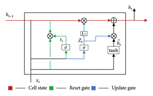
The green line in the figure represents the update gate.
()
2.
The blue line in the picture represents the reset door.
()
3.
Candidate hidden state:
()
4.
Hidden layer state:
()

Figure 1 introduces the internal structure of GRU, ⊗ represents the Kronecker product between vectors, ⊕ represents vector addition, and the subscript t represents the time index. Formulas (9)–(12) are the detailed calculation formulas of GRU network structure, where lowercase letters represent variables and uppercase letters represent matrices. , , , and k = z, r, h represent the weight matrix and deviation parameters of the input vector x_t and the hidden state vector h_t in different gates, respectively.

Details are in the caption following the image — **Figure 1**
Open in figure viewer PowerPoint

GRU network structure chart.

2.4. CEEMDAN-VMD-GRU Model

The number of GRU layers is generally set to below four, and the number of cells is set to below 200 because excessive layers or cells can lead to significantly increased computational time, while the prediction accuracy is only slightly improved [23]. Therefore, in order to make the GRU model have better expression ability and computational efficiency, the GRU model designed in this study adopts a three-layer network structure with 128, 64, and 32 units, respectively, from top to bottom. In addition, the GRU model designed in this study adopts a three-layer network structure with 128, 64, and 32 units from top to bottom. To enhance the performance of the network, a dropout layer with a dropout rate of 0.5 is incorporated after each network layer, along with a dense layer for output. This approach aims to enhance the network’s ability to handle overfitting and improve generalization. The model is optimized using the Adam optimizer, with the mean square error (MSE) serving as the loss function. Tanh is employed as the activation function for all layers. The initial learning rate is set at 0.001, employing a batch size of 32, while enabling data shuffling. The training process is set to 100 epochs. To further accelerate the computation, a learning rate adaptive strategy is introduced with a patience value of 10 epochs. This means that if the loss value of the validation set does not decrease for 10 consecutive epochs, the learning rate will be adaptively reduced to ten percent of the current value. To prevent overfitting, a patience value of 50 epochs is set for early stopping. This means that if the loss value does not decrease after 50 epochs, the model will stop training early. For parameter details, please refer to Appendix B (Table A2).

The flowchart of Figure 2 illustrates the hybrid prediction model proposed in this paper, which combines the CEEMDAN, VMD, and GRU techniques. The following steps outline specific processes:

1.
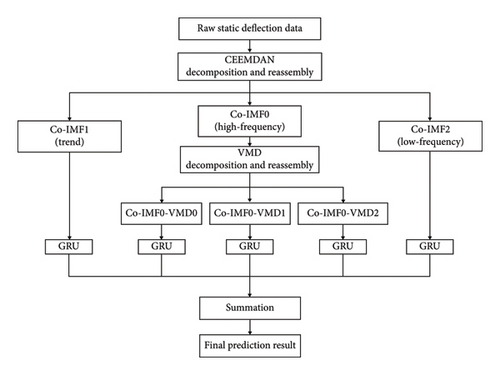
Primary modal decomposition: Using CEEMDAN to decompose and recombine the deflection data of SHM, three components are obtained: high-frequency sequence, trend sequence, and low-frequency sequence.
2.
Secondary mode decomposition: Performing secondary modal decomposition using VMD on the high-frequency sequence obtained from the primary modal decomposition of CEEMDAN yields three additional components.
3.
The GRU model is constructed to learn the characteristics of these five components, capture their internal change patterns, and predict their corresponding deflection values. Ultimately, the predicted results of each individual component are combined to yield the ultimate prediction for deflection.

2.5. Model Evaluation

This paper utilizes the Metrics function from the Scikit-learn module to evaluate the model’s performance. The evaluation metrics employed include the determination coefficient (R²), the root mean square error (RMSE), the mean absolute error (MAE), and the mean absolute percentage error (MAPE), as shown in formulas (13)–(16). The symbol y_i is employed to represent the original value, while the symbol

represents the predicted value, and the symbol

denotes the average value of the original dataset. In the condition where y_i is zero, the value of ε is deliberately chosen as a small positive number to prevent the denominator from being zero.

()

2.6. Data Normalization

In this study, the MinMaxScaler function from the Scikit-learn module is utilized for normalizing the deflection data, as shown in formula (17). y represents the deflection data, and y_min and y_max correspond to the minimum and maximum values of the deflection data, respectively. After normalizing the deflection data, it is scaled within the range of [0, 1] and becomes dimensionless.

()

3. Data Preprocessing

3.1. Data Sources

The experimental data in this paper are sourced from the SHM system installed on a cable-stayed bridge. This system accurately captures deflection data from three specific sections of the main span: the 1/4 section, the midspan section, and the 3/4 section and the sampling rate is 1 Hz. In the data collection stage, some deflection data of these three sections were collected from March to May. The specific time and position of the sample data are shown in Table 1. In this paper, the deflection data of the 1/4 section of the main span from 12:00 to 14:00 on March 15, 2023, are taken as an example to prove that the proposed CEEMDAN-VMD-GRU model can achieve a high-precision prediction effect, and then the data of different measuring points and different time periods are used to verify the robustness of the improved model. The ratio of the training set to the validation set is 8:2.

Table 1. Sample data comparison table.

Condition	Time period	Duration (h)	Location
1	2023-03-15 12:00∼2023-03-15 14:00	2	1/4 section
2	2023-05-05 04:45∼2023-05-05 08:45	4	3/4 section
3	2023-05-24 02:00∼2023-05-24 10:00	8	Midspan section
4	2023-05-25 04:00∼2023-05-25 16:00	12	1/4 section
5	2023-03-14 14:20∼2023-03-15 14:20	24	Midspan section
6	2023-04-09 00:00∼2023-04-11 00:00	48	3/4 section

3.2. CEEMDAN Primary Decomposition and Sample Entropy Recombination

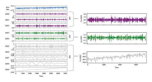
Taking the deflection data of the main span 1/4 section collected from 12: 00-14: 00 on March 15, 2023, as an example, the CEEMDAN function in the python EMD-signal module is used to adaptively decompose the selected sample data. The raw deflection data are decomposed into nine IMFs and one residue (referred to as IMF9 in this paper). According to Z. Liu and H. Liu’s study [31], the combination of IMFs that have similar sample entropy values effectively reduces computational complexity, enhances modeling efficiency, and mitigates overfitting problems. Therefore, this section uses the sample entropy function in the Python sampen module, sets the threshold r = 0.1 and the dimension m = 1 to calculate the entropy of the nine IMFs and one residual, and uses the KMeans function in the sklearn.cluster module to classify data with similar entropy values. Because the vehicle load, temperature effect, and structural damage are distributed in three frequency domains of high, medium, and low, the number of clusters is set to 3, and three types of data are obtained: high frequency sequence Co-IMF0 (IMF0∼2), trend sequence Co-IMF1 (IMF3∼4), and low-frequency sequence Co-IMF2 (IMF5∼9).

In Figure 3, the left side illustrates the raw deflection data in blue, the high-frequency component in violet, the trend component in green, and the low-frequency component in gray. The time of deflection monitoring data is represented on the horizontal axis in seconds, and the values of each component are represented on the vertical axis in millimeters. The right side of Figure 3 is the result of sample entropy recombination. Through observation, it is found that Co-IMF0 has the highest complexity and the most significant fluctuations, followed by Co-IMF1, and both of their values are concentrated around 0. The complexity of the Co-IMF2 is the lowest, but it exhibits significant variations.

3.3. VMD Secondary Decomposition and Recombination

By using the GRU model to predict the components of CEEMDAN after primary decomposition and recombination, it is found that the prediction accuracy of Co-IMF0 is 60%, that of Co-IMF1 is 99%, and that of Co-IMF2 is 95%. Consequently, it becomes imperative to conduct a secondary modal decomposition on the Co-IMF0 to enhance the prediction accuracy of the GRU model. Referring to the literature of Yuan et al. [32], since EMD, EEMD, and CEEMDAN belong to the same series of methods, using them again to decompose and predict the Co-IMF0 will not yield better results. When extracting time-frequency features using VMD, the concentration phenomenon of the frequency band in the high-frequency component feature is more pronounced compared to CEEMDAN. This approach effectively mitigates the problem of feature mixing. Consequently, VMD is employed in this paper to perform a secondary decomposition of Co-IMF0.

This paper employs CEEMDAN decomposition technology instead of VMD decomposition technology for the primary decomposition and recombination because the sum of the individual IMF components after VMD decomposition and recombination does not match the raw data. The value of Co-IMF0 is small, and the recombination error after VMD decomposition can be basically ignored. The vmdpy module in Python is used to complete the VMD decomposition operation of Co-IMF0. The decomposition effect of VMD is mainly influenced by the selection of the modal number (k) value. However, determining the optimal value of k currently poses a challenge as no practical or reliable method exists for this purpose. Therefore, this section investigates the impact of VMD on the decomposition and recombination prediction of Co-IMF0 by exploring various values of k. As shown in Figure 4, when k = 9, MAPE is the lowest and R² is close to 1. Therefore, the parameter k = 9 is selected in this paper. In addition, the other initial parameters of VMD are Alpha = 2000, Init = 1, DC = 0, Tau = 0, and Tol = 1e − 7. Considering that predicting each of the 9 components obtained from the VMD decomposition of Co-IMF0 will significantly increase computation time, sample entropy and K-means are further used for classification and recombination, resulting in 3 new components (Co-IMF0-VMD0∼2), as shown in Figure 5.

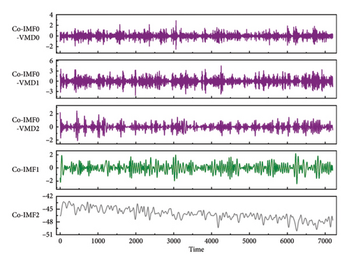
Table 2 shows the specific details of using the CEEMDAN-VMD-GRU improved model to decompose and reconstruct the deflection data. For components with disparate value ranges (Co-IMF0-VMD0~2 and Co-IMF1~2), RMSE, and MAE were calculated using normalized data. Under the hyperparameter configuration of epochs=100 and patience=10, the reconstructed model achieved an overall test performance of R² = 0.953, RMSE=0.327, MAE=0.257, and MAPE=0.58%, with a computational time of 2702 seconds. These results suggest that the model can predict the deflection data well and has certain practical value.

Table 2. CEEMDAN-VMD secondary decomposition prediction results.

Method	R²	RMSE	MAE	MAPE (%)	Time/n
Co-IMF0-VMD0	0.964	0.013	0.010	2.18	494
Co-IMF0-VMD1	0.986	0.011	0.008	1.83	508
Co-IMF0-VMD2	0.976	0.015	0.010	2.06	409
Co-IMF1	0.995	0.009	0.005	1.12	437
Co-IMF2	0.902	0.038	0.025	2.46	536
Final	0.953	0.327	0.257	0.58	2702

Note: Parameters: runs = 20, epochs = 100, and patience = 10.

4. Comparative Analysis

4.1. Comparison of Different Decomposition Methods

This section utilizes the EMD, EEMD, and CEEMDAN functions in the Python EMD-signal module for decomposing the deflection monitoring data. The prediction performance of GRU is compared across various decomposition methods to determine the optimal approach. To eliminate the influence of sample entropy, this part excludes the recombination step performed after using the adaptive decomposition method to decompose the deflection data. Due to different decomposition methods, the number of obtained IMFs also varies. EMD generates 10 IMFs, EEMD generates 11 IMFs, and CEEMDAN generates 10 IMFs. Additionally, the predictor employs early stopping mechanism. Therefore, a rough comparison of computation time is conducted by dividing the time by the number of IMF components. The prediction results can be found in Table 3. Because EEMD is unable to eliminate the added white noise, there is a significant disparity between the recombined data and the raw data, resulting in negative R² values. Results after 20 iterations indicate that CEEMDAN is more suitable for decomposing and predicting the deflection data.

Table 3. Comparing different decomposition methods using the GRU model.

Method	R²	RMSE	MAE	MAPE (%)	Time/n
EMD	0.654	0.909	0.812	1.8	318
EEMD	−540.096	34.653	34.652	43.1	328
CEEMDAN	0.711	0.824	0.721	1.6	330

Note: Parameters: runs = 20, epochs = 100, and patience = 10.

4.2. Comparison of Different Models

Table 4 shows the performance results for the deep neural network (DNN), LSTM, and GRU models with the same network structure under the single prediction framework, as well as the CEEMDAN-GRU and CEEMDAN-VMD-GRU models under the decomposition and recombination prediction framework. This paper employs a combination approach that utilizes decomposition methods and neural network models to represent an improved model. For example, CEEMDAN-VMD-GRU represents an enhanced model in which the data are decomposed and recombined using CEEMDAN and VMD methods before being predicted individually using the GRU model. Because of the presence of the early stopping mechanism, the predictor may complete training without finishing all 100 epochs, resulting in a shorter computational time compared to the theoretically required time for complete training.

Table 4. Comparison of different prediction models.

Model	R²	RMSE	MAE	MAPE (%)	Runtime
Single-DNN	0.539	1.102	0.932	2.1	42
Single-LSTM	0.661	0.945	0.774	1.8	518
Single-GRU	0.667	0.937	0.770	1.7	352
CEEMDAN-GRU	0.804	0.650	0.499	1.1	1833
CEEMDAN-VMD-GRU	0.953	0.327	0.257	0.6	2702

Note: Parameters: runs = 20, epochs = 100, and patience = 10.

From Table 4, it can be observed that, for a single predictive framework model, GRU and LSTM perform similarly, and both outperform DNN. Furthermore, GRU has a shorter computing time. Therefore, the selection of the GRU model as the research object in this study can enhance the hybrid model’s prediction performance and computational efficiency. The results of using the CEEMDAN-GRU improved model outperform all other single models in terms of prediction accuracy. This indicates that utilizing the CEEMDAN decomposition technique to decompose and recombine the deflection data can enhance the predictive capabilities of the GRU model. However, the accuracy of the CEEMDAN-GRU model is about 80%, indicating that the model cannot fully explain the variability of the target variable, that is, the deflection data after CEEMDAN decomposition and reorganization still exhibit high complexity, and the model cannot capture the change of deflection data. When the deflection data suddenly increase or decrease, the prediction performance is poor. Moreover, the RMSE is 0.650 and MAE is 0.499, indicating that the prediction accuracy of the CEEMDAN-GRU model is insufficient, emphasizing the need for further model optimization. Therefore, based on the CEEMDAN primary decomposition, this paper introduces the VMD secondary decomposition technology. Through the process of decomposing the high-frequency sequence once more, the complexity is diminished, leading to an improvement in the model’s prediction accuracy. When epochs = 100 and patience = 10, running it 20 times and taking the average value, the prediction index of CEEMDAN-VMD-GRU is as follows: R² = 0.953, RMSE = 0.327, and MAE = 0.257. It is considered that the model can predict the deflection data well. Comparing the CEEMDAN-GRU model of CEEMDAN decomposition and sample entropy recombination in this section with the model that only decomposes and does not reorganize in Section 4.1, it can be found that using sample entropy to reorganize the data can improve the prediction performance.

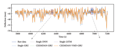
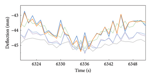
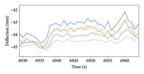
Figure 6 shows the prediction effect comparison of five models: Single-DNN, Single-LSTM, Single-GRU, CEEMDAN-GRU, and CEEMDAN-VMD-GRU. Extract the relatively better-predicted part (b) and the relatively worse part (c) from graph (a). As shown in part (b), compared to the other four models, the prediction results of the CEEMDAN-VMD-GRU model are in good agreement with the original deflection data, which is consistent with the results presented in Table 4. The prediction results of the CEEMDAN-VMD-GRU model in this dataset are significantly different from those of other models, demonstrating that the model outperforms the others in terms of prediction accuracy. In part (c), although the prediction accuracy of the CEEMDAN-VMD-GRU model is relatively lower, its trend remains consistent, which is in contrast to the obvious lag of other models in trend recognition. Therefore, in general, the CEEMDAN-VMD-GRU model shows superior performance in accurately predicting and capturing the trend changes of deflection data compared with the other four models.

4.3. Model Robustness Verification

To further validate the performance of the improved CEEMDAN-VMD-GRU model proposed in this study on different deflection datasets, this section uses the data with serial numbers 1–6 mentioned in Section 3.1 (see Table 1) for verification. Because the deflection data from different time periods are affected by temperature, they will show different value ranges. Therefore, the prediction results for different data in Table 5 cannot be directly compared, but the values of RMSE, MAE, and MAPE are close to 0, while R² is close to 1. This proves that the model has a very high prediction accuracy. Figures 7(a), 7(b), 7(c), 7(d), 7(e), and 7(f) show the prediction results of the improved CEEMDAN-VMD-GRU model for the six groups of deflection datasets at different time periods. Additionally, they display the probability density distribution of each group of datasets, in which the orange part represents the repair data. The deflection data distributions in Figures 7(a), 7(b), and 7(d) are relatively concentrated, with a range of 20∼30 mm, and the overall range of change is small. The deflection data distribution of Figures 7(c), 7(e), and 7(f) is relatively dispersed, with a range of 60∼120 mm. The overall range of change is large. The research shows that the enhanced model provides accurate predictions for the values and trends of deflection data with different distributions (Table 5).

Table 5. The prediction results of different measuring point data.

Condition	R²	RMSE	MAE	MAPE (%)
1	0.952	0.333	0.255	0.6
2	0.946	0.203	0.134	1.1
3	0.997	0.166	0.115	0.5
4	0.982	0.194	0.133	0.7
5	0.996	0.514	0.395	1.4
6	0.978	0.969	0.762	1.5

5. Conclusion

In this paper, the missing data interpolation task is transformed into a time series prediction task, and a high-precision repair model of bridge SHM missing data based on CEEMDAN-VMD two-stage modal decomposition and GRU DL is proposed. The model relies only on historical monitoring data and is independent of variable correlation and adjacent sensors. Compared with other monitoring data repair methods based on DL in the field of bridge health monitoring, this model can not only repair large-scale complex data through prediction but also effectively address the nonlinearity and nonstationarity in the original deflection data. By comparing the three decomposition methods of EMD, EEMD, and CEEMDAN and the five models of Single-DNN, Single-LSTM, Single-GRU, CEEMDAN-GRU, and CEEMDAN-VMD-GRU, the following conclusions are drawn:

1.
Using CEEMDAN for decomposing deflection data and predicting yields better results than using EMD and EEMD for decomposition and prediction. Compared to CEEMDAN, VMD can effectively reduce the complexity of signals for components with higher feature complexity, making it easier for the model to track.
2.
Incorporating sample entropy for the classification and recombination of the decomposed components leads to an enhanced prediction accuracy of the GRU model.
3.
CEEMDAN-VMD-GRU performs well in predicting the deflection data. Compared to the Single-GRU model, it shows a 27.41% improvement in R², a 49.69% decrease in RMSE, a 48.50% decrease in MAE, and a 48.21% decrease in MAPE. It is suitable for repairing missing deflection data in bridge SHM.

Although this study demonstrates the effectiveness of the CEEMDAN-VMD-GRU model, there are still some limitations and further research ideas. This method only discusses the influence of using data from the same type of measuring points at different positions as input features for the neural network model on the prediction performance of the CEEMDAN-VMD-GRU model. It is suggested that future research can further study the use of the data of different types of measuring points at the same position as input, such as the correlation between deflection data and strain data, temperature data, vibration data, and other data. Additionally, in the univariate repair method based on the combination of quadratic decomposition and neural network models, this study does not consider using different neural network models and structures for the components obtained through decomposition and recombination. It may be beneficial to explore various neural network models and structures tailored to the specific characteristics of different components.

Conflicts of Interest

The authors declare no conflicts of interest.

Author Contributions

All authors have made equivalent contributions to this study.

Funding

This work was supported by the National Natural Science Foundation of China (Grant No. 52178486).

Acknowledgments

This study did not receive any dedicated funding from public, commercial, or nonprofit organizations.

Appendix A: Hardware and Compilation Environment

Table A1. Hardware and compilation environment.

Hardware	Version
Central processing unit (CPU)	12th Gen Intel(TM) i7-12700
Random access memory (RAM)	16G 3200 MHZ
Operating system (OS)	Windows 10 Professional × 64
Graphics processing unit (GPU)	Intel(R) UHD Graphics 770
Programming language	Python 3.8.17
Development environment	Anaconda3 2020.07
Deep learning framework	TensorFlow 2.5.0

Appendix B: Hyperparameters and Explanations

Table A2. Hyperparameters and explanations.

Hyperparameters	Value	Description
Dropout	0.2	A regularization technique that removes hidden layer units according to a certain probability to prevent overfitting
Epochs	100	The total number of iterations performed on the complete dataset is crucial for adjusting model parameters to enhance performance
Batch size	32	The number of samples contained in each batch when performing gradient descent
Validation split	0.2	Divide the proportion of training set and validation set
Shuffle	True	Whether to randomly disrupt the order of training data before the start of each training cycle
Activate	Tanh	An activation function, which maps the input to the range [−1, 1], helps to deal with the vanishing gradient problem
Optimizer	Adam	The weights of a neural network are efficiently updated by the commonly utilized optimization algorithm, which combines the first-stage gradient moment estimation and the second-stage moment estimation
Callbacks	N/A	This paper utilizes the ReduceLROnPlateau and EarlyStopping in Keras to enhance the performance of the mechanism model
Run	20	As the noise added during the decomposition process is random, the performance of the model in this paper is assessed by averaging multiple runs
Patience	10	The early stopping mechanism reduces the learning rate when the verification loss value exceeds 10 epochs without improvement and stops the operation when the verification loss value exceeds 50 epochs without improvement

Open Research

Data Availability Statement

Data are available upon reasonable request to the authors.

References

1 Xu D., Xu X., Forde M. C., and Caballero A., Concrete and Steel Bridge Structural Health Monitoring—Insight into Choices for Machine Learning Applications, Construction and Building Materials. (2023) 402, https://doi.org/10.1016/j.conbuildmat.2023.132596.
10.1016/j.conbuildmat.2023.132596
Web of Science® Google Scholar
2 Zhou X. and Zhang X., Thoughts on the Development of Bridge Technology in China, Engineering. (2019) 5, no. 6, 1120–1130, https://doi.org/10.1016/j.eng.2019.10.001.
10.1016/j.eng.2019.10.001
CAS Web of Science® Google Scholar
3 Kullaa J., Detection, Identification, and Quantification of Sensor Fault in a Sensor Network, Mechanical Systems and Signal Processing. (2013) 40, no. 1, 208–221, https://doi.org/10.1016/j.ymssp.2013.05.007, 2-s2.0-84881316942.
10.1016/j.ymssp.2013.05.007
Web of Science® Google Scholar
4 Li Y., Huang H., Zhang W., and Sun L., Structural Full-Field Responses Reconstruction by the SVD and Pseudo-Inverse Operator-Estimated Force With Two-Degree Multi-Scale Models, Engineering Structures. (2021) 249, https://doi.org/10.1016/j.engstruct.2021.112986.
10.1016/j.engstruct.2021.112986
Web of Science® Google Scholar
5 Chen C., Tang L., Lu Y. et al., Reconstruction of Long-Term Strain Data for Structural Health Monitoring With a Hybrid Deep-Learning and Autoregressive Model Considering Thermal Effects, Engineering Structures. (2023) 285, https://doi.org/10.1016/j.engstruct.2023.116063.
10.1016/j.engstruct.2023.116063
Web of Science® Google Scholar
6 Li Z., Li A., and Han X., Dynamic Analysis and Experimental Study of Variations of the Dynamic Parameters of the Runyang Suspension Bridge, China Civil Engineering Journal. (2010) 43, no. 4, 92–98, https://doi.org/10.15951/j.tmgcxb.2010.04.002.
10.15951/j.tmgcxb.2010.04.002
Google Scholar
7 Fan G., Li J., and Hao H., Dynamic Response Reconstruction for Structural Health Monitoring Using Densely Connected Convolutional Networks, Structural Health Monitoring. (2021) 20, no. 4, 1373–1391, https://doi.org/10.1177/1475921720916881.
10.1177/1475921720916881
Web of Science® Google Scholar
8 Jiang K., Han Q., and Du X., Lost Data Neural Semantic Recovery Framework for Structural Health Monitoring Based on Deep Learning, Computer-Aided Civil and Infrastructure Engineering. (2022) 37, no. 9, 1160–1187, https://doi.org/10.1111/mice.12850.
10.1111/mice.12850
Web of Science® Google Scholar
9 Zhang J., Huang M., Wan N., Deng Z., He Z., and Luo J., Missing Measurement Data Recovery Methods in Structural Health Monitoring: the State, Challenges and Case Study, Measurement. (2024) 231, https://doi.org/10.1016/j.measurement.2024.114528.
10.1016/j.measurement.2024.114528
Web of Science® Google Scholar
10 Fan G., Li J., and Hao H., Lost Data Recovery for Structural Health Monitoring Based on Convolutional Neural Networks, Structural Control and Health Monitoring. (2019) 26, no. 10, https://doi.org/10.1002/stc.2433, 2-s2.0-85070687577.
10.1002/stc.2433
PubMed Web of Science® Google Scholar
11 Tang Z., Bao Y., and Li H., Group Sparsity-Aware Convolutional Neural Network for Continuous Missing Data Recovery of Structural Health Monitoring, Structural Health Monitoring. (2021) 20, no. 4, 1738–1759, https://doi.org/10.1177/1475921720931745.
10.1177/1475921720931745
Web of Science® Google Scholar
12 Lei X., Sun L., and Xia Y., Lost Data Reconstruction for Structural Health Monitoring Using Deep Convolutional Generative Adversarial Networks, Structural Health Monitoring. (2021) 20, no. 4, 2069–2087, https://doi.org/10.1177/1475921720959226.
10.1177/1475921720959226
Web of Science® Google Scholar
13 Chen C., Tang L., Lu Y. et al., Temperature-Induced Response Reconstruction Method Based on DL-AR Model and Attention Mechanism, Structures. (2023) 50, 359–372, https://doi.org/10.1016/j.istruc.2023.02.044.
10.1016/j.istruc.2023.02.044
Web of Science® Google Scholar
14 Jiang K., Han Q., Du X., and Ni P., Structural Dynamic Response Reconstruction and Virtual Sensing Using a Sequence to Sequence Modeling With Attention Mechanism, Automation in Construction. (2021) 131, https://doi.org/10.1016/j.autcon.2021.103895.
10.1016/j.autcon.2021.103895
Web of Science® Google Scholar
15 Deng Y., Ju H., Zhai W., Li A., and Ding Y., Correlation Model of Deflection, Vehicle Load, and Temperature for In-Service Bridge Using Deep Learning and Structural Health Monitoring, Structural Control and Health Monitoring. (2022) 29, no. 12, https://doi.org/10.1002/stc.3113.
10.1002/stc.3113
PubMed Web of Science® Google Scholar
16 Entezami A. and Shariatmadar H., Structural Health Monitoring by a New Hybrid Feature Extraction and Dynamic Time Warping Methods Under Ambient Vibration and Non-Stationary Signals, Measurement. (2019) 134, 548–568, https://doi.org/10.1016/j.measurement.2018.10.095, 2-s2.0-85056217597.
10.1016/j.measurement.2018.10.095
Web of Science® Google Scholar
17 Li L., Zhou H., Liu H., Zhang C., and Liu J., A Hybrid Method Coupling Empirical Mode Decomposition and a Long Short-Term Memory Network to Predict Missing Measured Signal Data of SHM Systems, Structural Health Monitoring. (2021) 20, no. 4, 1778–1793, https://doi.org/10.1177/1475921720932813.
10.1177/1475921720932813
Web of Science® Google Scholar
18 Entezami A. and Shariatmadar H., Damage Localization Under Ambient Excitations and Non-Stationary Vibration Signals by a New Hybrid Algorithm for Feature Extraction and Multivariate Distance Correlation Methods, Structural Health Monitoring. (2019) 18, no. 2, 347–375, https://doi.org/10.1177/1475921718754372, 2-s2.0-85060999452.
10.1177/1475921718754372
Web of Science® Google Scholar
19 Sarmadi H., Entezami A., and De Michele C., Probabilistic Data Self-Clustering Based on Semi-Parametric Extreme Value Theory for Structural Health Monitoring, Mechanical Systems and Signal Processing. (2023) 187, https://doi.org/10.1016/j.ymssp.2022.109976.
10.1016/j.ymssp.2022.109976
Web of Science® Google Scholar
20 Liang Z., Gao M., Chen B., Yuan Y., and Song Y., F. Zhao, Prediction Model of Deflection Based on Wavelet and LSTM+GAN, 5th International Conference on Computer Information Science and Application Technology (CISAT 2022), 2022, Chongqing, China, SPIE, https://doi.org/10.1117/12.2656835.
10.1117/12.2656835
Google Scholar
21 Xin J., Zhou C., Jiang Y., Tang Q., Yang X., and Zhou J., A Signal Recovery Method for Bridge Monitoring System Using TVFEMD and Encoder-Decoder Aided LSTM, Measurement. (2023) 214, https://doi.org/10.1016/j.measurement.2023.112797.
10.1016/j.measurement.2023.112797
Web of Science® Google Scholar
22 Han Y., Mi L., Shen L. et al., A Short-Term Wind Speed Prediction Method Utilizing Novel Hybrid Deep Learning Algorithms to Correct Numerical Weather Forecasting, Applied Energy. (2022) 312, https://doi.org/10.1016/j.apenergy.2022.118777.
10.1016/j.apenergy.2022.118777
Web of Science® Google Scholar
23 Zhou F., Huang Z., and Zhang C., Carbon Price Forecasting Based on CEEMDAN and LSTM, Applied Energy. (2022) 311, https://doi.org/10.1016/j.apenergy.2022.118601.
10.1016/j.apenergy.2022.118601
Web of Science® Google Scholar
24 Li K., Huang W., Hu G., and Li J., Ultra-Short Term Power Load Forecasting Based on CEEMDAN-SE and LSTM Neural Network, Energy and Buildings. (2023) 279, https://doi.org/10.1016/j.enbuild.2022.112666.
10.1016/j.enbuild.2022.112666
Web of Science® Google Scholar
25 Jujie W., Xin S., Qian C., and Quan C., An Innovative Random Forest-based Nonlinear Ensemble Paradigm of Improved Feature Extraction and Deep Learning for Carbon Price Forecasting, The Science of the Total Environment. (2020) 762.
Google Scholar
26 Wu Z. and Huang N. E., Ensemble Empirical Mode Decomposition: A Noise-Assisted Data Analysis Method, 2008.
Google Scholar
27 Torres M. E., Colominas M. A., Schlotthauer G., and Flandrin P., A Complete Ensemble Empirical Mode Decomposition With Adaptive Noise, 2011 IEEE International Conference on Acoustics, Speech and Signal Processing (ICASSP), 2011, https://doi.org/10.1109/ICASSP.2011.5947265, 2-s2.0-80051634709.
10.1109/ICASSP.2011.5947265
Google Scholar
28 Dragomiretskiy K. and Zosso D., Variational Mode Decomposition, IEEE Transactions on Signal Processing. (2014) 62, no. 3, 531–544, https://doi.org/10.1109/TSP.2013.2288675, 2-s2.0-84893418756.
10.1109/TSP.2013.2288675
Web of Science® Google Scholar
29 Hochreiter S. and Schmidhuber J., Long Short-Term Memory, Neural Computation. (1997) 9, no. 8, 1735–1780, https://doi.org/10.1162/neco.1997.9.8.1735, 2-s2.0-0031573117.
10.1162/neco.1997.9.8.1735
CAS PubMed Web of Science® Google Scholar
30 Cho K., Merrienboer B., Bahdanau D., and Bengio Y., On the Properties of Neural Machine Translation: Encoder-Decoder Approaches, 2014.
Google Scholar
31 Liu Z. and Liu H., A Novel Hybrid Model Based on GA-VMD, Sample Entropy Reconstruction and Bilstm for Wind Speed Prediction, Measurement. (2023) 222, https://doi.org/10.1016/j.measurement.2023.113643.
10.1016/j.measurement.2023.113643
Web of Science® Google Scholar
32 Yuan L., Wang C., Wang F., and Jia L., TCN Short-Term Water Level Prediction Based on CEEMDAN-VMD Time-Frequency Double Layer Feature Extraction, 2022 7th International Conference on Computational Intelligence and Applications (ICCIA), 2022, 128–134, https://doi.org/10.1109/ICCIA55271.2022.9828441.
10.1109/ICCIA55271.2022.9828441
Google Scholar

All articles

A Novel Bridge Deflection Missing Data Repair Model Based on Two-Stage Modal Decomposition and Deep Learning

Abstract

1. Introduction