1. Introduction

Tunnels constitute vital components of transportation systems, facilitating connectivity and promoting economic development [1, 2]. Due to the effects of complex geological and operational conditions, tunnel structures are subjected to diverse and dynamic forces, necessitating continuous monitoring for structural health [3, 4]. The imperative of ensuring tunnel safety and mitigating potential risks has led to the emergence of tunnel early-warning research based on the massive number of monitoring data. By proactively identifying potential anomalies and structural issues, it enables timely intervention, preventing disasters, and ensuring the long-term stability of tunnel structures [5, 6]. This research of early warning is essential for enhancing the resilience and reliability of tunnel structural health monitoring (SHM) systems, minimizing risks, and ultimately contributing to sustainable urban development and transportation safety.

Tunnel early-warning research operates at the intersection of structural engineering, data science, and risk management [7–9]. The goal is to fortify existing monitoring systems with predictive capabilities, enabling timely response to emerging structural anomalies [10]. Early-tunnel-warning methods primarily relied on approaches such as statistics, fuzzy mathematics, and expert systems [11, 12]. These methods often require the determination of a necessary safety factor, but there is currently no universal method or basis for determining this factor, and empirical or semi-empirical theories play a significant role during this process. Consequently, when faced with complex working conditions or changes in those conditions, the precision of these methods is significantly reduced. Since numerical simulation methods can effectively model the mechanical response characteristics of structures under complex conditions, applying extreme load conditions to numerical models has become a new approach to determine warning thresholds [13]. However, simplifications and assumptions made during the modeling process lead to a certain degree of deviation between the numerical results and real values. With the continuous development of artificial intelligence technologies, developing data-driven warning models has become a current trend [14, 15]. Some researches focused on data-based have been reported to achieve this goal [16, 17]. For example, the principal component analysis method has been widely used to identify the key disaster-causing factors during the failure process of rocks [18], and the anomaly detection in long-term tunnel deformation monitoring [19]. The support vector machines had been adopted for risk evaluation of tunnel convergence based on the prediction results [20].

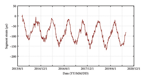
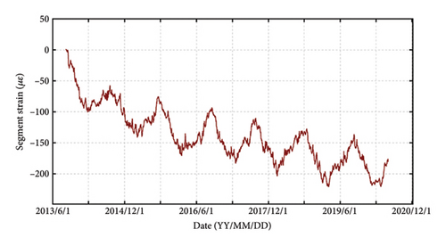
These researches made great effort in promoting the development of early-warning system. However, the challenges in tunnel early-warning research are multifaceted [21, 22]. These methods still lack sufficient capability to learn the nonlinear mechanical response characteristics of structures, and the absence of physical mechanism constraints results in insufficient learning of the hidden spatiotemporal correlations in the data. As a result, the level of intelligence in current tunnel warning methods urgently needs further improvement [23]. Specifically, the early-warning values reliant on data-based are usually set to a constant, which are insufficient in addressing the dynamic and evolving nature of tunnel environments. In fact, the mechanical responses of tunnel structure are nonlinear with period variation trend [24, 25], as shown in Figure 1. Therefore, the early-warning system would be failure using a constraint early value if a significant anomaly occurred but its amplitude is not enough to exceed the early-warning value. Additionally, previous research has generally been limited to warning only one spatial position of tunnel structure. However, the variation magnitude of tunnel structure varied with spatial positions, as shown in Figures 1(a) and 1(b). The early-warning analysis aimed to the spatial difference is rarely reported. Hence, a paradigm shift toward real-time monitoring, data-driven algorithm, and mechanical responses characteristics has become imperative in tunnel early-warning analysis [26].

Initially, the framework and methodology of the proposed model are introduced and formulated using monitoring data acquired from a representative underwater shield tunnel. Subsequently, accurate predictions are made for the evolving trends of structural behaviors and their corresponding probabilities by incorporating insights gained from the temporal and spatial correlations of structural mechanical responses. Ultimately, differentiated alert thresholds for different spatial positions are determined based on these predictions. Furthermore, a set of variation experiments is undertaken to validate the robustness and reliability of the proposed model. Through the convergence of cutting-edge technologies and interdisciplinary collaboration, this research devoted to identify potential anomalies of tunnel structure before they threaten the integrity of these vital components of urban transportation systems, striving to promote the intelligent level of tunnel management.

2. Proposed Model

In this section, the problem of spatial dynamic early warning was formalized firstly. Then, the framework to solve this problem was presented, and the methodology in framework was introduced in detail. To describe the proposed model, all notations used in this paper are listed in Table 1.

2.2. Framework of the Prewarning Method

A prewarning model comprises three main components: position encoding module, conditional distribution prediction module, and cyclic sampling module based on predicted mean and variance, which was proposed. The structure of DL-AR model, which is supposed to capture the temporal relationships inherent in the sensors and the correlated information among different positions, is shown in Figure 2.

In the position encoding module, the positional information of sensors was extracted from the original data and embedded into a distributional space, yielding an embedding matrix:

$$ ()

where each $$ denotes the embedded feature vector for sensor i, m is the total number of sensors, and d is the feature dimension. Then, the embedding matrix E recorded the position features of all sensors was connected with the monitoring data matrix X to generate a new series and was fed into the conditional distribution prediction module, which was built upon seq2seq structure, consisting of an encoder and a decoder constructed using long short-term memory(LSTM) cells. Based on the μ and σ generated by the hidden state of different layers in LSTM cell, a Gaussian distribution was developed in the cyclic sampling module to obtain the current prediction results through random sampling. Subsequently, the current results progress forward as the new input to predict the mechanical behaviors until the entire prediction range concludes. After a series of repeated experiments and statistical analysis, the probability of each prediction results was determined. As a result, the threshold range of early warning was determined according to the prediction results and the probability.

2.3. Methodology of the Proposed Model

2.3.1. Deep Autoregression Algorithm DL-AR

In essence, the DL-AR model is an enhanced LSTM method. LSTM method is a kind of recurrent neural network (RNN). The emergence of LSTM networks addresses the problems of gradient vanishing and exploding existed in the classical RNN model by introducing gating units, forget gates, and cell states to regulate the flow of information [27, 28]. This method is superior to handle long sequential data and capturing long-term dependencies [29], so that it was adopted in this study to capture the temporal correlations and predict the future evaluation trend of tunnel structure. The prediction process of DL-AR model is displayed in Figure 3.

Regarding our established model, the monitoring data $$ were processed using a linear transformation to add the embedded information of sensor positions as follows [30]:

$$ ()

The resulting matrix is then input into LSTM cells, allowing the model to consider the positional information of sensors, expressed as follows

$$ ()

where f_t, i_t, $$, C_t, o_t represent the forget gate, input gate, new cell state, current cell state, and output gate, respectively. δ denotes the sigmoid activation function, and ⊙ represents element-wise multiplication. W_f, W_i, W_C, W_o are the weight matrices for the gate units, while b_f, b_i, b_C, b_o are their corresponding bias terms.

The encoder and decoder are designed as the same architectures, but the term “conditioning range” was used to denote the encoding range, which corresponds to the time period [t₀ − g + 1,  t₀ − 1 ], and the term “prediction range” was used to represent the decoding range, which corresponds to the time period [t₀, t₀ + q] [31]. As shown in Figure 3, when t is within the conditioning range, the input values are denoted by $$, and while during the prediction range, the LSTM cell at time step t generates μ and σ using the hidden state h_t through different linear layers as follows

$$ ()

$$ ()

where $$ represents the mean and $$ represents the standard deviation of the conditional distribution at time step t, $$ denotes the concatenation of hidden states, $$ and $$ are weight matrices used for linear transformations, $$ and $$ are the corresponding bias terms, respectively. Since the variances σ in the Gaussian distribution are always positive, we take the Softplus activation function, defined as Softplus(x) = log(1 + e^x) for the linearly transformed variances to ensure they remain positive.

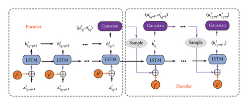
Based on the values of μ_t and σ_t, Gaussian distribution was developed to obtain the current prediction results $$ through random sampling. Subsequently, this value serves as the input $$ according to Equation (3) for the prediction of next moment, recursively predicting the output at t + 1 moment until the entire prediction range concludes. To obtain the entire sampling result and derive the probability distribution, the entire decoding phase would iterate k times using the h_t−1 from the conditioning range for prediction. Statistics are then conducted on the different random results to represent the probability distribution.

2.3.2. Optimization for Objective Function

To ensure that the predicted distribution fits the prediction range more effectively, a specific objective function should be designed to maximize both the likelihood of the sample data and the probability of the samples in the prediction range.

Let $$ denote the ground truth measurement for sensor i at time t (with $$), and let $$ and $$ are the predicted mean and standard deviation at this moment, respectively. Define n_q = m × q, where m is the total number of sensors and q is the number of prediction time steps. Therefore, the L_MAE (MAE loss) is adopted to maximize the likelihood of the sample data, expressed as follows:

$$ ()

In addition, maximum-likelihood estimation was adopted to maximize the probability of the samples in the prediction range. The log-probability density function (PDF) of a normal distribution and the negative log-likelihood L_lh are given by

$$ ()

$$ ()

According to equations (8)–(10), the optimized objective function $$ of the proposed prewarning models can be determined by integrating these two losses, as follows:

$$ ()

where λ ∈ [0, 1] is a regularization parameter that balances the contribution of the two loss components.

2.3.3. Evaluation Metrics for Model Performance

Two metrics are used in this work to evaluate the performance of the proposed method, including root-mean-square error (RMSE) and Pearson correlation coefficient (PCC).

RMSE is widely used to calculate the error between prediction results and truth values. Let $$ denote the median predicted value for sensor i at time t and $$ denote the corresponding ground truth. Then, the RMSE is defined as

$$ ()

where n_q = m × q is the total number of prediction points.

PCC is used to evaluate the correlation between prediction results and truth data. A larger positive PCC indicates a stronger similarity in trend between the predictions and the ground truth. The PCC is calculated as

$$ ()

where $$ represents the average of the ground truth values, and $$ represents the average of the predicted values.

Following Seeger et al. [32], the ρ-risk (quantile risk) is employed to characterize the accuracy of the uncertainty range of predictions. In this context, let $$ denote the ρ-quantile of the predicted distribution for sensor i at time t. The asymmetric deviations are defined as

$$ ()

where

$$ ()

and

$$ ()

3. Background for a River Tunnel

As a case study, we utilized monitoring data from a SHM system installed in a representative underwater shield tunnel to instantiate the DL-AR model. This section introduces the dataset sources, encompassing geological conditions and the monitoring scheme.

3.1. Geological Conditions

The Wuhan Yangtze River Tunnel, situated in Hubei, China, stands as the first underwater shield tunnel crossing the Yangtze River. The tunnel comprises two lines, east line and west line, with a total length of 3.63 km, incorporating a 1080-m land connection segment and a 2550-m river-crossing segment. The geological conditions in the area exhibit significant variations in longitudinal load. Specifically, the river-crossing section encounters primary geological layers, including clay, silty clay, silt, silty-fine sand, medium-coarse sand, pebble, and pelitic siltstone mixed sand shale. Approximately 80% of the tunnel is excavated in silty-fine sand, medium-coarse sand, and pebble, as shown in Figure 4. The tunnel is constructed using segmental lining, with external and internal diameters of 11 and 10 m, respectively. Owing to factors such as high water pressure and complex ground conditions, the tunnel is prone to structural issues during its long-term operation.

3.2. Real-Time Monitoring in the Site

To assess the operational safety of the lining structure and implement the intelligent management of the Wuhan Yangtze River Tunnel, a SHM system has been deployed in the field. This system comprises 12 monitoring sections, with six sections on each of the east and west lines, and their locations and geological characteristics are depicted in Figure 5 and Table 2. Additionally, at each monitoring section, four strain gauges are installed, with two positioned on the arch crown and two on the arch shoulder, as shown in Figure 6. The system commenced service in July 2013, and to date, it has been operating smoothly, providing reliable real-time monitoring data for structural stability analysis and alertness studies.

Table 2. Characteristics of the determined monitoring sections.

Section number	Characteristics
W1 and E1	On the side of the Hankou bank, where the strata change greatly
W2 and E2	Abrupt change in the longitudinal slope o near to Hankou bank
W2 and E2	Flat section of the shield in the center of river
W2 and E2	Minimum overburden in the center of river
W2 and E2	Abrupt change in the longitudinal slope near to Wuchang bank
W2 and E2	Large slope and near the land side

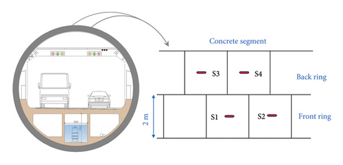
The monitoring data obtained from the SHM system of Wuhan Yangtze River tunnel were adopted to conduct experiments. As an example, the strain monitoring data in one section, from June 1, 2019, to May 20, 2020, were derived with a sampling frequency of one day. Therefore, the monitoring dataset used for experiment contains four time series, and each time series contains 335 samples, expressed as X ∈ R^4×335.

4. Prediction of the Future Mechanical Behaviors of Tunnel Structure

In this section, the proposed DL-AR model was instantized on the strain monitoring data obtained from the study case to predict the evolution trend of tunnel structure. To verify the reliability of the predicted results, the robustness and superiority of the DL-AR model were discussed, respectively.

4.2. Reasonability for Model Internal Structure

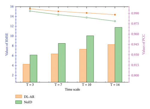
One of the highlights of the proposed model is the consideration of the spatial heterogeneity effect on the mechanical response of tunnel structures, thereby enhancing traditional warning methods. To demonstrate the validity of incorporating spatial heterogeneity, a prediction model named “NoID” is established, which disregards this factor. The structure of this model is identical to the DL-AR model, except for the direct input of monitoring data into LSTM for encoding learning in the former, compared to the spatial feature learning conducted prior to inputting data into the LSTM model in the latter. This indicated that the input information of NoID model is $$. Furthermore, the hyperparameter settings remain consistent between the two models. Taking forecast time scales of 3, 7, 10, and 14 days as examples, the impact of spatial heterogeneity on the predictive capabilities of these two models is illustrated in Figure 7. It is evident that while the predictive abilities of both models diminish with increasing forecast time scales, the agreement between the predictions of the DL-AR model and the actual states surpasses that of the NoID model at any time scale, with lower errors. Specifically, the error is decreased as least 2 με while the correlations improved over 0.3% after considering the spatial heterogeneity effect, and the superiority of the model becomes more obvious with the increase of prediction time scale. Consequently, spatial heterogeneity emerges as a crucial factor in the structural mechanical response, significantly enhancing the predictive capability of the model when considered.

4.3. Reliability With Other Commonly Used Methods

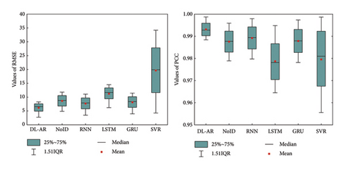
To validate the reliability of the presented DL-AR model, a comparison analysis is conducted with widely used models, including RNN, classical long short-term memory (LSTM), gated recurrent unit (GRU), and support vector regression (SVR). The data experiments of all models under multiple time scales (ranging from 1 to 14 with a step of 1) are carried out, and the experimental results are displayed in Figure 8. The box boundary represents the distribution range of error and correlations of different models, where a larger range indicates poorer stability and lower robustness of the model. Additionally, the red label represents the average RMSE and PCC values for each model across the 14 time scales. Clearly, the DL-AR model is more stable than others, with the smallest RMSE and PCC ranges among all models.

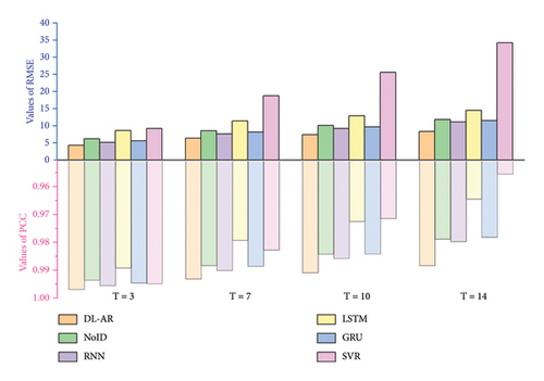
Furthermore, specific evaluation results for the predictive capabilities of different models at time scales of 3, 7, 10, and 14 are derived, as depicted in Figure 9. It is evident that all models exhibit similar characteristics, with predictive performance declining as the time scale increases. However, the predictive ability of the DL-AR model stands out significantly compared to others. The consistency between the prediction results with the actual data is near to 99% even under the prediction scale of 14 days. The RNN model follows closely behind DL-AR, benefitting from its adeptness at capturing temporal correlations and excelling in short-term learning. Conversely, the predictive ability of the SVR model is the weakest, indicating challenges in capturing the complex temporal and spatial correlations inherent in the time series data. In contrast to SVR model, the consistency of DL-AR model improved about 5%. Consequently, the proposed DL-AR model emerges as a reliable choice.

5. Determination of the Spatial Dynamic Prewarning Values

The reliable prediction result is the essential to determine the precise threshold range of early warning. Due to uncontrollable factors at the site, the evolution trend of structural states will also change accordingly. Taking the next 14 days as an example, the warning thresholds for the evolution trend of structural states are shown in Figure 10. From the figure, it can be seen that the warning values determined by the model proposed in this paper are dynamic and exhibit distinct temporal characteristics. In the figure, the dashed lines represent the range of states that the structure may exhibit under random disturbances, and the solid red line indicates the states that are most likely to occur. States within the range of the dashed line are considered normal and will not trigger warnings. Conversely, the white area outside the dashed line represents the warning zone. The probability of the structure exhibiting this state under normal disturbances is extremely low, and its occurrence will trigger a warning.

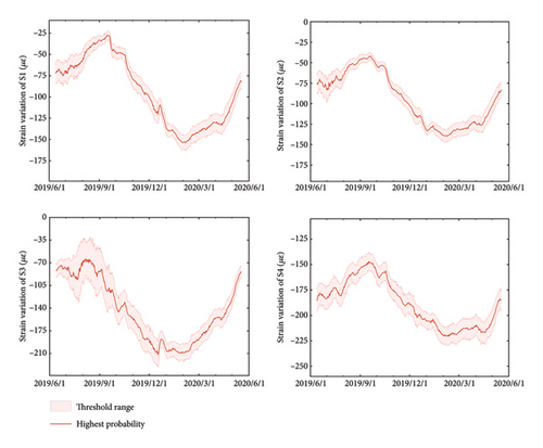
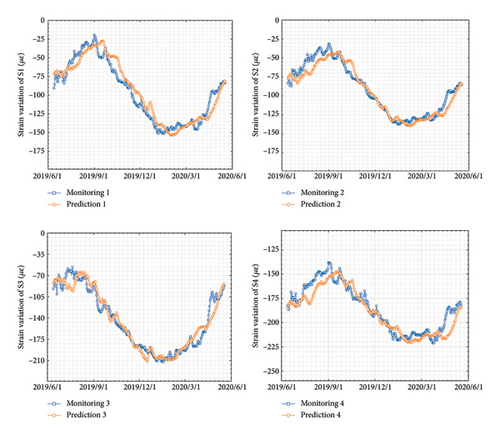
Furthermore, the evolution trend of the structural states predicted by this model is compared with the monitoring results on site, as shown in Figure 11. Obviously, the predicted evolution trend aligns well with the actual structural states. The prediction accuracy for the structural states over the next 3, 7, 10, and 14 days is presented in Table 3. Clearly, the predictive capability of the model decreases with increasing prediction time scale. This is because, with a larger time scale, there is a greater probability of unforeseen disruptive factors occurring, which in turn increases the likelihood of the structure deviating from its normal evolution trend. Nonetheless, the prediction error for the structural evolution trend within the next 14 days using the proposed model is less than 8.28 με, with a match rate of 98.8% compared to actual results.

6. Conclusions

In this study, a novel prewarning method named DL-AR was proposed for detecting structural anomalies in underwater shield tunnels using deep autoregression techniques. By considering the spatial variations in structural mechanical responses and dynamically adjusting the prewarning range based on the evolving structural behaviors, the accuracy and efficiency of early-warning technology were significantly enhanced. The main conclusions of the study are summarized as follows:

DL-AR, an enhanced LSTM model, incorporates an embedding layer and a linear layer to handle input and output information, respectively. The determination of threshold ranges is constitutionally to predict the future mechanical behaviors and assess the probability of various states of tunnel structures using the spatiotemporal correlations captured by the DL-AR model. Anomalies are defined as occurrences below a probability of less than 10%. Consequently, refined threshold ranges are determined for different positions within the tunnel structure, rather than adopting a universal range for all positions. Not only for underwater shield tunnel, the proposed model is applicable for other engineering with nonlinear and dynamic mechanical behaviors.

As a case study, the DL-AR model was applied to the Wuhan Yangtze River tunnel to identify segment strain anomalies. A series of experiments were conducted to verify the reliability of model, including the reasonability of internal structure and comparing its performance with other commonly used models. The experimental results demonstrated an improved prediction accuracy for structural mechanical evaluation when considering spatial correlations. The prediction results showed near to 99% consistency with actual data, a 5% enhancement compared to classical models. The precise prediction of future mechanical behaviors of tunnel structures ensures the reliability of early-warning results, thereby establishing the credibility of the DL-AR model.

Despite its effectiveness in identifying structural anomalies in tunnel segment strain, evaluating the stability of the overall tunnel structure remains a significant challenge due to its complexity and numerous contributing factors. It is essential to conduct this research in the near future.

Conflicts of Interest

The authors declare no conflicts of interest.

Funding

This work is supported by the National Key R&D Program of China under grant 2023YFB2603605 and 2021YFC3100805, the Fundamental Research Funds for the Central Universities of China under grant JKF-20240769, the National Natural Science Foundation of China under grant U2469205, 42293355, and 51991392, Key project in Hubei Province under grant 2023BCB048, and the Science and Technology Planning Project of Tibet Autonomous Region of XZ202201ZY0021G.