Structural Control and Health Monitoring

Volume 2025, Issue 1 4684985

Research Article

Open Access

A Novel Nonlinear Output-Only Damage Detection Method Based on the Prediction Error of PCA Euclidean Distances Under Environmental and Operational Variations

Jiezhong Huang

orcid.org/0009-0005-7366-3184

Department of Civil and Intelligent Construction Engineering , Shantou University , Shantou , Guangdong Province, China , stu.edu.cn

Anhui Provincial International Joint Research Center of Data Diagnosis and Smart Maintenance on Bridge Structures , Chuzhou University , Chuzhou , Anhui, China , chzu.edu.cn

MOE Key Laboratory of Intelligent Manufacturing Technology , Guangdong Engineering Center for Structure Safety and Health Monitoring , Shantou University , Shantou , Guangdong Province, China , stu.edu.cn

Search for more papers by this author

Sijie Yuan,

Sijie Yuan

orcid.org/0009-0000-2455-6968

Department of Civil and Intelligent Construction Engineering , Shantou University , Shantou , Guangdong Province, China , stu.edu.cn

Search for more papers by this author

Dongsheng Li,

Dongsheng Li

orcid.org/0000-0001-8143-4449

Department of Civil and Intelligent Construction Engineering , Shantou University , Shantou , Guangdong Province, China , stu.edu.cn

Shantou Key Laboratory of Offshore Wind Energy , Shantou University , Shantou , Guangdong Province, China , stu.edu.cn

Search for more papers by this author

Tao Jiang,

Corresponding Author

Tao Jiang

[email protected]

orcid.org/0000-0001-8031-1287

Department of Civil and Intelligent Construction Engineering , Shantou University , Shantou , Guangdong Province, China , stu.edu.cn

Shantou Key Laboratory of Offshore Wind Energy , Shantou University , Shantou , Guangdong Province, China , stu.edu.cn

Search for more papers by this author

Jiezhong Huang,

Jiezhong Huang

orcid.org/0009-0005-7366-3184

Department of Civil and Intelligent Construction Engineering , Shantou University , Shantou , Guangdong Province, China , stu.edu.cn

Anhui Provincial International Joint Research Center of Data Diagnosis and Smart Maintenance on Bridge Structures , Chuzhou University , Chuzhou , Anhui, China , chzu.edu.cn

Search for more papers by this author

Sijie Yuan,

Sijie Yuan

orcid.org/0009-0000-2455-6968

Department of Civil and Intelligent Construction Engineering , Shantou University , Shantou , Guangdong Province, China , stu.edu.cn

Search for more papers by this author

Dongsheng Li,

Dongsheng Li

orcid.org/0000-0001-8143-4449

Department of Civil and Intelligent Construction Engineering , Shantou University , Shantou , Guangdong Province, China , stu.edu.cn

Shantou Key Laboratory of Offshore Wind Energy , Shantou University , Shantou , Guangdong Province, China , stu.edu.cn

Search for more papers by this author

Tao Jiang,

Corresponding Author

Tao Jiang

[email protected]

orcid.org/0000-0001-8031-1287

Department of Civil and Intelligent Construction Engineering , Shantou University , Shantou , Guangdong Province, China , stu.edu.cn

Shantou Key Laboratory of Offshore Wind Energy , Shantou University , Shantou , Guangdong Province, China , stu.edu.cn

Search for more papers by this author

First published: 18 February 2025

https://doi.org/10.1155/stc/4684985

Academic Editor: Francesc Pozo

Share a link

Email
Wechat
Bluesky

Abstract

Vibration-based damage detection relies on changes in structural dynamic features. However, environmental and operational variations (EOVs) can cause changes in dynamic features that mask those caused by damage. In addition, the EOV effects on dynamic features are often nonlinear, which limits the application of many linear damage detection methods. A novel nonlinear output-only method is proposed to address this. This method leverages variational mode decomposition (VMD) as a preprocessing step to remove seasonal patterns and noise from the modal frequencies. The first modes of the decomposition results (IMF1 signals) are then used to calculate the Euclidean distance based on the residual obtained by the principal component analysis (PCA) method. To eliminate the nonlinear EOV effects and provide normalized damage features for reliable continuous dynamic monitoring, a Gaussian process regression (GPR) model is trained to learn the underlying calculation rule of the PCA Euclidean distance. Due to the linear nature of PCA, the nonlinear EOV effects are still retained in both the PCA Euclidean distance and the GPR–predicted value. Through a subtraction process, their common nonlinear environmental effects can be removed, and the resulting prediction error can serve as a normalized feature sensitive to structural damage. The proposed method is validated through a simulated 7-DOF example and real data from the Z24 bridge, with several comparisons highlighting its effectiveness.

1. Introduction

With the rapid development of sensing technologies [1], signal processing techniques [2], and machine learning [3], vibration-based damage detection methods have received increasing attention in recent years. Fan et al. presented a comprehensive review of vibration-based damage identification methods and conducted comparative studies [4]. Hou et al. [5] and Avci et al. [6] reviewed the latest advancements in vibration-based damage identification for civil engineering structures. In summary, the basic idea behind vibration-based methods is that structural damage causes changes in the dynamic properties of structures, such as frequencies and mode shapes. Therefore, structural damage can be detected by solving an inverse problem based on changes in these dynamic features.

However, most vibration-based damage detection methods are successfully applied to numerical and laboratory models but rarely used for actual structures. The main reason is that the dynamic features of civil structures are sensitive not only to structural damage but also to environmental and operational variations (EOVs), such as temperature [7, 8], humidity [9], wind speed [10], and traffic loading [11]. For example, the frequency variation ratio of an arch bridge in Shenzhen caused by EOVs was reported to be up to 5% [12]. Similarly, the natural frequencies of the Z24 bridge fluctuated significantly due to changing temperature conditions [13]. Although these changes induced by EOVs might appear innocuous, they can overwhelm the changes in dynamic features caused by structural damages, leading to false alarms. Therefore, it is essential to consider the EOV effects while developing reliable vibration-based damage detection methods [14, 15].

Researchers have adopted several approaches to consider the EOV effects in vibration-based damage detection, which can be categorized as input–output or output-only approaches [16]. The former is based on measuring both the environmental/operational data (e.g., temperature) and structural dynamic features (e.g., modal frequencies), while the latter relies only on measured dynamic features [17]. Input–output methods attempt to establish the relationship between the measured environmental factors and dynamic features using a regression model and then extract the model residuals as the damage indicator insensitive to environmental influences. Common input–output methods include linear regression [18], polynomial regression [19], the autoregressive model with exogenous input [20], Bayesian linear regression [21], support vector regression [7], random forest models [22] Gaussian process regression (GPR) [23] switching response surface models [24], and artificial neural networks [25]. However, the potentially influential environment variables should be comprehensively considered to establish an accurate input–output relationship. In practice, it may not be possible to measure all influential input variables for civil structures [26]. Therefore, output-only methods are often more beneficial for removing the effects of EOVs.

Output-only methods assume that the changes in dynamic features caused by EOVs are different from those caused by damage and aim to extract a damage indicator insensitive to EOVs from structural dynamic features. The widely used output-only methods include principal component analysis (PCA) [18, 27], Johansen cointegration [28, 29] factor analysis [30], second-order blind identification [31], singular spectrum analysis [32], missing data analysis [33], and state-space autoregressive model [34]. However, most of these methods are linear, assuming a linear relationship between monitored dynamic features. Nonlinear relationships between modal frequencies are observed in multiple real bridges during long-term monitoring, such as the Z24 bridge [13], Dowling Hall Footbridge [19], and the KW51 bridge [18]. In such scenarios, the effectiveness of linear damage detection methods is limited. To address such nonlinearities and facilitate the damage detection, some nonlinear output-only methods are proposed, such as autoassociative neural networks [26, 35], nonlinear narrow dimension techniques [36], GMM with MSD method [37], manifold learning approaches [38], regime-switching cointegration method [39, 40], switching independent component analysis (ICA) [41], and several clusterwise nonlinear methods [42, 43]. Mousavi et al. recently developed a nonlinear method based on variational mode decomposition (VMD), cointegration, and recurrent neural networks. The superiority of the proposed method was demonstrated by an experimental example of the Z24 bridge [44]. Daneshvar et al. [45] proposed a locally discriminative reconstruction-based dictionary learning algorithm for removing nonlinear environmental effects and used the Mahalanobis-squared distance to determine damage indices for SHM. Sarwar et al. [46] introduced a probabilistic temporal autoencoder methodology for overcoming the environmental and operational impacts, detecting potential damage of a monitored bridge by applying an exponentially weighted moving average filter and a chart-based threshold mechanism.

PCA is one of the most widely used output-only methods for damage detection under changing environments. The basic concept of PCA is to remove the variance due to environmental effects. By eliminating this variance, the loss of information (i.e., reconstruction error) via projection and remapping is used to compute a Euclidean distance for damage detection [28, 47]. Due to its simplicity and straightforward interpretability, the PCA-based damage detection method has been successfully applied in various types of structures, such as wind turbines [48], bridges [18], frame structures [49], and historic bell towers [50]. Moreover, to address the issue of insufficient training data leading to inaccurate PCA models, Jin et al. proposed an adaptive PCA that dynamically updates reference [51]. To diminish the effect of outliers in establishing a reliable PCA model, robust PCA was used to clean the training data in a separate preprocessing step [18, 52]. Recently, Ma et al. [53] developed an anomaly detection algorithm based on probabilistic PCA, which can be used to detect the presence of damage under various data-missing conditions. However, these PCA variants are essentially linear methods that struggle to remove nonlinear environmental influences [54].

Local PCA [55] and subdomain PCA [56] were proposed to overcome this nonlinear limitation. These methods divide the data into multiple subdomains using a clustering algorithm, and then PCA is performed for each subdomain. However, this category of methods has limited applicability because it assumes that the nonlinear relationship between the data must be bilinear or multisegment linear. In addition, the parameter values involved must be carefully chosen to yield accurate damage detection results. Furthermore, another nonlinear version of PCA, kernel PCA (KPCA), has been proposed to remove nonlinear environmental effects [57]. In this method, the original data are nonlinearly mapped to a high-dimensional feature space using the kernel trick, transforming it into linearly correlated data. Linear PCA is then applied to the mapped data. Since the specific form of the nonlinear mapping function is not required, KPCA applies to any nonlinear data. However, the selection of the kernel function and kernel parameters significantly impacts the detection results, and thus determining the optimal parameters remains an open problem.

In this paper, a new nonlinear PCA damage detection method under EOVs was proposed. This method first calculates the Euclidean distance of PCA residuals using the conventional PCA method (i.e., PCA Euclidean distance) and then employs the GPR model to learn the underlying calculation rule of the PCA Euclidean distance. Due to the linear nature of the PCA method, the nonlinear environmental effects are still retained in the PCA Euclidean distance. Similarly, the Euclidean distance predicted by the GPR model also includes the nonlinear environmental effects. By subtracting the GPR–predicted Euclidean distance from the PCA Euclidean distance, their common nonlinear environmental effects are removed. Therefore, the GPR prediction error is insensitive to nonlinear EOVs. In addition, to improve the prediction accuracy of the GPR and the EOV separation accuracy of PCA, the VMD method is employed to denoise and remove seasonal patterns in the original data. To test the method developed in this paper, a numerical 7-DOF model and the Z24 bridge are analyzed. Moreover, the proposed method is compared with some state-of-the-art methods, such as PCA, cointegration, PCA–GPR, and VMD–PCA–LSTM. The results demonstrate that the method developed in this paper performs better than the other methods.

2. Contributions

The main contributions and novelty of this research can be summarized as follows:

i.
Development of an innovative damage detection method: This research introduces a novel method specifically designed for long-term SHM under varying environmental conditions. The key innovation lies in the integration of VMD, PCA, and GPR. This approach effectively addresses environmental variability, including nonlinear effects, which most traditional normalization techniques (such as MSD, PCA, and factor analysis) can only handle in a linear context.
ii.
Preprocessing with VMD to enhance data quality: A critical element of our method is the application of VMD for preprocessing, which helps to denoise signals and remove seasonal patterns. By improving data quality, this step optimizes the performance of the GPR model, which is used to predict PCA Euclidean distances. As a result, the accuracy of damage detection is significantly improved.
iii.
Damage detection through prediction error analysis: In relation to the third contribution, it brings the key novel part of this paper. The proposed method seeks to learn the rules behind the calculation of the PCA Euclidean distances, through training an GPR on signals obtained from the healthy state. As the GPR has not learned the effect of damage on these distances, the prediction errors of these values will increase significantly once damage occurs. Moreover, since PCA is a linear method, residual nonlinear environmental effects are present in both the PCA distances and the GPR predictions. However, by calculating the prediction error, these nonlinear effects are effectively removed. This method improves upon previous work, such as Mousavi et al.’s approach using RNNs for predicting Johansen cointegration residuals [44]. Unlike their approach, which is sensitive to the selection of cointegration residuals and can lead to inaccurate results, this research leverages GPR to learn PCA Euclidean distances without the need for residual selection, and it is shown that GPR has a higher prediction accuracy than RNN.

3. PCA

PCA is a statistical technique used for dimensionality reduction in data analysis. It transforms a large set of correlated variables into a smaller set of uncorrelated variables called principal components (PCs), which retain most of the variance present in the original dataset. These PCs are linear combinations of the original variables and are orthogonal (uncorrelated) to each other. The first PC captures the most variance in the data, the second captures the second most, and so on. In the field of SHM, PCA is widely used for damage detection under varying environmental conditions. The procedure for using PCA in damage detection is briefly introduced as follows [27].

Consider a measured damage feature matrix Z_d×n, where n represents the number of sample points and d represents the number of damage features. To extract the data information related to the environmental effects, the measured features Z are first projected into a lower space through a linear mapping [58].

()

where T_d×q is called the loading score and the dimension q may be considered as the number of combined environmental factors that affect the features. Generally, T can be obtained by extracting the main q eigenvectors of the covariance matrix of the original data. Alternatively, a more practical method is to perform a singular value decomposition in the covariance matrix:

()

where U is an orthonormal matrix, and the columns of U represent the eigenvectors of the covariance matrix and Σ is a diagonal matrix, which is composed of singular values σ₁, σ₂, ⋯, σ_d, and each singular value represents the contribution of the corresponding PC to the variance of the data. In general, only a few major EOVs (e.g., temperature) significantly affect the damage features, while others (e.g., noise) have negligible influence and can be ignored. Therefore, the first q singular values corresponding to major EOVs are significantly larger than the others [59],

()

Subsequently, by remapping the projected data back into the original space, the damage features dominated by environmental influences (i.e., reconstructed damage features) can be obtained as follows:

()

Furthermore, the reconstruction errors can be computed as follows:

()

From the error vector E_k obtained at time t_k, the novelty index (NI) is defined using the Euclidean distance [17] as

()

Therefore, the PCA Euclidean distance is used as a damage indicator that is insensitive to changing EOVs. Although PCA has been widely used for removing environmental effects, it is fundamentally a linear tool that assumes a linear relationship between damage features [27] In practice, the EOV effects are often nonlinear, resulting in a nonlinear relationship between damage features. Consequently, the effectiveness of PCA is limited in such scenarios [55].

4. Theoretical Backgrounds of VMD–PCA–GPR–Based Damage Detection Methods

4.1. GPR

GPR is a nonparametric, probabilistic model used for regression tasks in machine learning. Built on the principles of Bayesian inference, GPR leverages the properties of Gaussian distributions to model underlying data. Unlike traditional regression models that specify a fixed form for the relationship between inputs and outputs, GPR assumes that the data can be described by a Gaussian process, any finite number of which have a joint Gaussian distribution. This approach allows for flexible modeling of complex, nonlinear relationships. For more information on GPR, readers can refer to [60]. In the proposed method, the GPR model is trained to learn the underlying rule behind the calculation of the PCA Euclidean distances.

4.2. VMD

VMD is an adaptive and intrinsic signal processing algorithm used to decompose complex, nonlinear, and nonstationary signals into a series of local vibrational modes known as intrinsic mode functions (IMFs) [61]. Conventional damage detection methods often struggle with changes in the variance of heteroscedastic data, complicating the detection process. Typically, this heteroscedasticity is caused by short-run stationary seasonal patterns under changing environments [62]. VMD is used in this paper to facilitate damage detection and eliminate the complex seasonal patterns in the applied signals before performing damage detection.

In general, the process of VMD can be considered as the construction and solution of a constrained variational problem, which can be expressed as follows [63]:

()

where N is the number of the IMF, u_k and ω_k are the kth IMF and its center frequency, f(t) is the original signal, δ(t) is the Dirac function, and ∗ is the convolution operation. ∂_t is the gradient function of t. To solve the constrained variational problem, a quadratic penalty term α and the Lagrangian multiplier λ are introduced to render the variational problem unconstrained [64] as follows:

()

Equation (8) can be solved by using the alternate direction method of multipliers (ADMMs). Initially, the decomposition mode number is predetermined. Each mode

in the Fourier domain, the corresponding center frequency

, and the Lagrangian multiplier λ are initialized. Subsequently, the modes

and the center frequencies ω_k are updated using equations (9) and (10), respectively [65].

()

where τ is the iteration number and f(ω), u(ω), and λ(ω) denote the Fourier transform of f(t), u(t), and λ(t), respectively. Then, following the same dual ascent step in the ADMM algorithm, the Lagrangian multiplier is updated, which can be expressed as follows [66]:

()

The above iteration continues until convergence is achieved, that is,

()

where the value ϵ is normally set as 10⁻⁶, and all IMFs can be recovered according to the above loop. In this paper, the VMD method is used to decompose the original frequency data into two IMFs [44] IMF1 corresponds to the nonstationary long-run pattern, while IMF2 corresponds to the short-run stationary seasonal pattern. By removing the seasonal patterns (IMF2), the retained IMF1 is used to calculate the PCA Euclidean distance.

4.3. Proposed VMD–PCA–GPR Method

Due to the linear nature of PCA, traditional PCA methods can produce false positives (FPs) and false negatives (FNs) under the influence of a nonlinear environment. To overcome the drawbacks of the linear PCA method, an improved method, namely, VMD–PCA–GPR, is proposed in this paper. The proposed damage detection method involves a three-step procedure: first, calculating the PCA Euclidean distance; second, learning the underlying rule for calculating the PCA Euclidean distance using the GPR method; and finally, obtaining a damage-sensitive indicator by subtracting the GPR–predicted Euclidean distance from the PCA Euclidean distance. Since PCA can only remove linear EOV effects, the nonlinear EOV effects remain in the PCA Euclidean distance, and its prediction value via GPR will naturally exhibit the same behavior. Consequently, the subtraction process can yield a small prediction error, allowing the removal of nonlinear EOV influences and providing a normalized damage indicator that reflects the structural changes caused by damage. Before performing the main damage detection procedure, VMD is employed as a data preprocessing tool for denoising and removing seasonal patterns in the signals, with the IMF1s being the output of the VMD. To provide a more comprehensive understanding of the algorithm’s stages, Figure 1 illustrates the flowchart of the proposed damage detection strategy.

Details are in the caption following the image — **Figure 1**
Open in figure viewer PowerPoint

Procedure of the proposed damage detection method.

In the offline training stage, the IMF1s, representing damage features, are used as input for the PCA algorithm to calculate the Euclidean distance according to equation (6). Following this, the GPR model is trained to capture the relationship between the IMF1 inputs (damage features) and their corresponding PCA Euclidean distances. However, due to the linear nature of PCA, it fails to fully account for the nonlinear environmental effects, which remain in both the PCA distances and the GPR predictions. By subtracting the predicted values from the PCA distances, we obtain a prediction error that effectively filters out these shared nonlinear environmental influences. To detect possible damage, an X-bar control chart can be constructed based on the prediction error in the training stage [63].

()

where UCL is the upper control limit in the X-bar control chart; μ_e and σ_e are the mean and standard deviation of prediction error in the training stage, respectively; and γ is taken as 3, corresponding to a confidence interval of 99.7%.

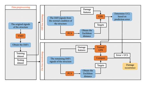
In the online monitoring stage, the trained GPR is used to predict the Euclidean distances of the test data. The outputs of the GPR are then compared against those obtained from the PCA algorithm utilizing the test data, and the prediction error of the GPR is calculated. Although the GPR model learns the calculation rules of PCA Euclidean distance under changing environments in the undamaged state, it cannot accurately predict the PCA Euclidean distance in the damaged state. Consequently, the prediction errors will increase significantly when damage occurs. Thus, if the prediction error exceeds the UCL, it indicates that the structure is damaged; otherwise, it suggests that the structure is undamaged.

5. Numerical Simulation: A 7-DOF Spring–Mass Model

In this study, a 7-DOF numerical example is utilized to validate the effectiveness of the proposed method. The 7-DOF system, illustrated in Figure 2, consists of a chain structure with both ends connected to the ground, and each lumped mass is 2 kg. To simulate the nonlinear environmental effects on the system, the relationship between stiffness and temperature is modeled as follows [17]:

()

for i = 1, 2, 4, 5, 6, 7, 8, and

()

where k_i is the stiffness of the ith spring and T represents the temperature. The temperature data from actual records in Beijing were utilized to simulate changing environmental conditions, which comprised 2189 sample points in 2013 and 239 sample points in March 2014, as depicted in Figure 3. To simulate structural damage, the stiffness of the second spring is reduced. In this study, two different damage cases are considered. In Damage case 1, the stiffness decreases in k₂ is 20% between sample points 2190 and 2310. In Damage case 2, the stiffness decreases in k₂ is 30% between sample points 2311 and 2428. Since each stiffness coefficient is a function of temperature, the natural frequencies related to temperature can be obtained by solving the generalized eigenvalue problem |M − ω²K(T)| = 0.

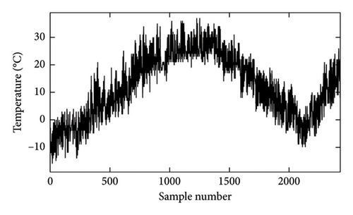
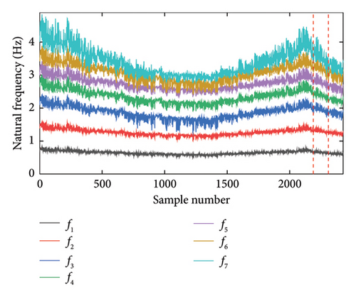
It is assumed that the natural frequencies of the system are contaminated by 2% Gaussian white noise. Figure 4 displays the seven natural frequency time series, with the two dashed vertical lines indicating the moments of damage occurrence. It can be observed that, due to temperature fluctuations, the relative change in these frequencies ranges from 2% to 6%. The temperature variations have induced substantial frequency changes, surpassing the magnitude of the damage effects. Therefore, solely observing frequency changes makes it challenging to identify damage, and it is necessary to eliminate the effect of temperature changes on frequency.

5.1. Damage Detection

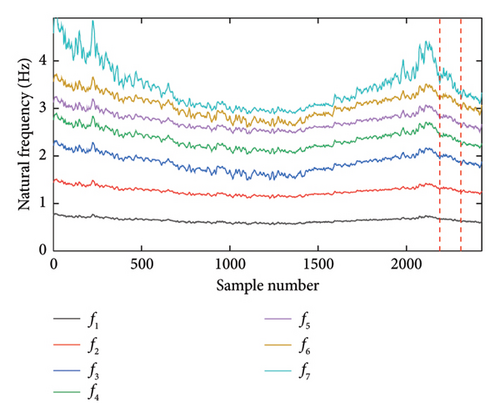
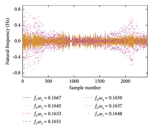
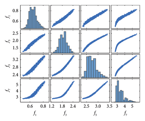
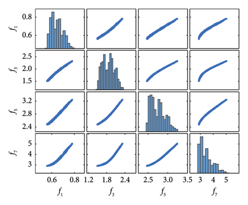
The first step of the proposed method is to separate seasonal patterns and noise in frequency data by the VMD. Two decomposed modes via VMD, the IMF1 and IMF2, are shown in Figure 5. It can be seen that the center frequencies of IMF1 signals are all zero, and the average center frequency of the IMF2 signals is about 0.165 cycles. Since the temperature data are sampled every 4 h, the corresponding frequency data are also sampled every 4 h. Consequently, the average center frequency of IMF2 is about 0.1647 cycles per 4 h, nearly equivalent to one complete cycle every 24 h. Therefore, the cyclical pattern of IMF2 represents the daily temperature variations, and these IMF2 signals are removed from the original frequency data [44] Moreover, Figure 6(a) shows the mutual codistribution between original frequencies, whereas Figure 6(b) shows the mutual codistribution between IMF1 signals. As shown in the off-diagonal plots, the relationship between frequencies is mutually nonlinear due to the bilinear relationship between stiffness and temperature, and the noise level is reduced after IMF2 signals are removed from the original frequencies. Moreover, it is observed that the distribution of frequencies in the main diagonal plots is non-Gaussian.

After removing the seasonal patterns (IMF2) from the original data, the IMF1 signals are utilized as the preprocessed frequency dataset for damage detection. In this study, 80% of the IMF1 signals from the normal condition are used as the training dataset. In comparison, the remaining 20% of the IMF1 signals from the normal condition, along with all observations of the damaged state, are used as the test data. In the offline training phase, the Euclidean distance of the residuals obtained by PCA is first calculated. Then, the GPR is trained to learn the calculation rule of the PCA Euclidean distance. The error between the GPR Euclidean distance and the PCA Euclidean distance is used to determine the upper control limit. During the online monitoring phase, the trained GPR model predicts the Euclidean distance using test IMF1 as the input, while the actual PCA Euclidean distance is also calculated. The prediction error can be determined by comparing the predicted values with the actual values. If the prediction error exceeds the UCL, it indicates potential damage in the structure.

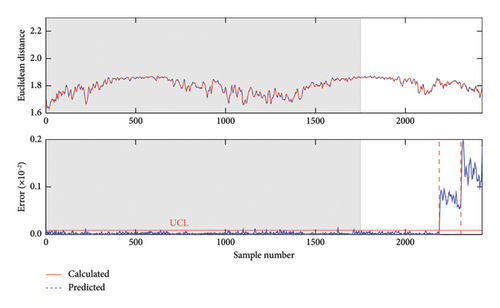
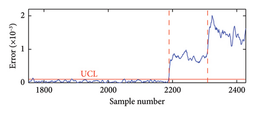
Figure 7 shows the damage detection result obtained by the proposed method, with the offline training phase indicated by the gray shading. It can be seen that the prediction error in the undamaged state remains stationary and is almost entirely below the control limit, with no severe environmental influences observed. This implies the proposed method’s effectiveness in detecting the normal condition and removing environmental effects. In contrast, nearly all the prediction errors for the damaged state significantly exceed the UCL line, with the prediction error increasing as the damage intensity grows. Due to the clear distinction between the damaged and normal conditions, the proposed method demonstrates excellent performance in damage detection for the 7-DOF system.

5.2. Comparison of the Proposed Method With Other Methods

Despite the accurate damage detection obtained by the proposed VMD–PCA–GPR method, this section conducts several comparative studies to demonstrate its superiority over some state-of-the-art techniques. These comparisons are divided into three parts. First, the proposed method was compared with the PCA and cointegration methods to demonstrate its excellent performance in handling nonlinear and non-Gaussian data. Second, since a critical step of the proposed method is to remove separate seasonal patterns using VMD, it is compared with the PCA–GPR method, which does not use VMD for data preprocessing. Finally, to illustrate the excellent predictive capability of the GPR model, the proposed method was compared with other popular prediction models.

In the first comparative study, Figures 8(a) and 8(b) show the damage detection results obtained using the PCA [27] and cointegration [67] methods. To ensure a fair comparison, VMD was used to preprocess the data before applying both PCA and cointegration. As observed, the damage detection result by PCA is severely affected by environmental variability, as most residuals in the undamaged state are nonstationary. In addition, the PCA residuals in the damaged state do not deviate from the control limit at all, leading to poor damage detection results. From Figure 8(b), it is evident that the cointegration method surpasses the PCA method in detecting the undamaged state. However, the cointegration residuals do not significantly deviate from the control limit in the damaged state, meaning the damage cannot be clearly detected. The main reason for their poor performance is the linear nature of the PCA and cointegration methods, which linearly project the original data to a new subspace. In practice, the frequencies of the 7-DOF system exhibit nonlinear correlations due to nonlinear environmental influences, which further affect the damage detection capabilities of the linear PCA and cointegration methods.

In the second comparative study, Figure 9 shows the damage detection result of the PCA–GPR method without VMD preprocessing. Significant variations and false alarms exist in the undamaged state, particularly between samples 1100 and 1200. Moreover, due to the effects of seasonal patterns and noise, the prediction error does not significantly increase with the degree of damage, implying that the detections of damage in Case 1 and Case 2 are not accurate enough. These observations indicate that seasonal patterns and noise seriously affect the performance of the PCA–GPR method and that reliable damage detection can be achieved by removing these effects using VMD.

In the last comparison regarding predictive models, the performance of the proposed GPR model is compared with that of the long short–term memory (LSTM) model. Figure 10 shows the damage detection results in the 7-DOF model using the VMD–PCA–LSTM method. As observed in Figure 10, although there are a few false alarms in the undamaged state, numerous FNs exist in the damage detection results. Due to the similarity of the prediction errors between the damaged and undamaged states, the VMD–PC–LSTM method exhibits low damage detectability. This conclusion indicates that the VMD–PCA–LSTM method is inferior to the proposed method in terms of prediction accuracy and damage detection performance. This may be because the LSTM predictive model is prone to issues such as gradient explosion or vanishing gradients due to its complex structure and deep network. In contrast, the GPR predictive model can effectively fit linear and nonlinear data while producing stable output results.

5.3. Effect of Frequency Grouping, Data Nonlinearity Degree, and Measurement Noise

To investigate the performance of the proposed method using different numbers of frequencies, Figure 11 presents the damage detection results using two frequencies [f₃, f₄] and three frequencies [f₁, f₃, f₅]. Note that only the damage detection results for the test phase are provided here. It can be seen that the proposed method can successfully identify the damage occurrences with varying numbers of frequencies, and the prediction error increases as the damage intensity grows. This confirms that the proposed method has excellent damage detection performance even when using a small number of frequency data.

As described in Section 3, the proposed method is a nonlinear method for separating environmental impacts and can be applied to situations where nonlinear relationships exist between frequencies. To investigate the effect of nonlinear intensity on the performance of the proposed method, an analysis was conducted on different nonlinearly correlated data. The nonlinear intensity of the data is determined by the variations in values a₁ and a₂ as described in equation (16). When a₁ and a₂ are equal, the relationship between the damage features is linearly correlated [17]. As the difference between a₁ and a₂ increases, it is assumed that the nonlinear intensity increases. Four nonlinear relationships are considered to examine the ability of the proposed method for damage detection of data with different nonlinear correlations, as shown in Table 1.

()

Table 1. Simulating different degrees of nonlinear relationships by setting different values of a₁ and a₂.

	k₃	k₁, k₂, k₄, k₅, k₆, k₇, k₈
Case 1	a₁ = −0.75, a₂ = −0.25, b₁ = 10, b₂ = 10	a₁ = −0.15, a₂ = −0.15, b₁ = 6, b₂ = 6
Case 2	a₁ = −1.00, a₂ = −0.25, b₁ = 10, b₂ = 10
Case 3	a₁ = −1.25, a₂ = −0.25, b₁ = 10, b₂ = 10
Case 4	a₁ = −1.50, a₂ = −0.25, b₁ = 10, b₂ = 10

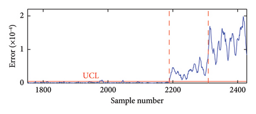
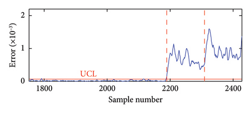
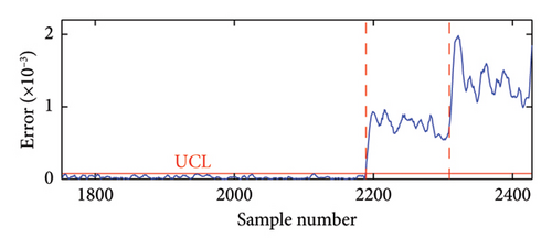
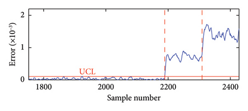
Figure 12 shows the performance of the proposed method in different nonlinear cases. As observed, the prediction error remains stationary for all nonlinear cases during the undamaged period but significantly jumps and exceeds the UCL line once damage occurs. In addition, even if the monitoring data exhibits a high degree of nonlinearity, the prediction error increases with the degree of damage. Thus, it can be concluded that the proposed method is insensitive to nonlinear environmental influences. This is because the nonlinear environmental influences are present in the PCA Euclidean distance and the GPR prediction. By subtracting the calculated PCA Euclidean distance from the predicted values, their common nonlinear environmental influences are removed, making the prediction error insensitive to these influences.

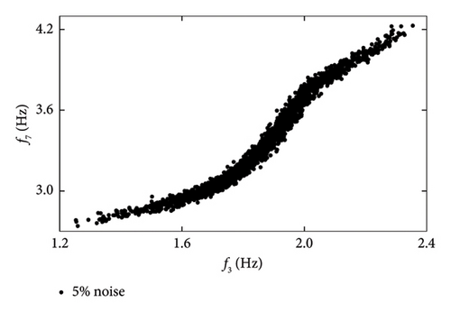
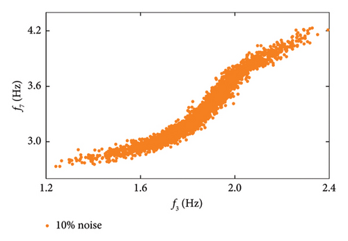
To assess the impact of measurement noise on the proposed method’s performance, frequency data with Gaussian white noise levels of 5%, 8%, and 10% were employed for damage detection. As illustrated in Figure 13, the correlation between frequencies f₃ and f₇ varies significantly at noise levels of 5% and 10%. Specifically, the correlation diminishes as the noise level increases from 5% to 10%, indicating that measurement noise adversely affects frequency correlation. To evaluate the effectiveness of the proposed method under varying noise levels, this study employs two key metrics: the false positive rate (FPR) and the false negative rate (FNR). These metrics provide insight into the method’s performance based on the following classifications: true positives (TPs), FPs, FNs, and true negatives (TNs). In the SHM context, a “positive” outcome indicates a damaged state, while a “negative” outcome signifies an undamaged state. A TN occurs when the structure is undamaged, and the method accurately identifies it. A FN arises when the structure is damaged, yet the method fails to detect it. Conversely, a FP happens when the structure is undamaged, but the method mistakenly identifies it as damaged. Lastly, a TP indicates that the structure is damaged, and the method successfully detects this, with NIs surpassing the threshold in the damaged state.

Table 2 displays the confusion matrix, offering a clear summary of TP, FP, FN, and TN. The FPR and FNR are defined in equations (17) and (18). To ensure reliable detection results, the damage detection process was conducted 20 times at each noise level. Table 3 presents the averaged FPR and FNR from these 20 detection trials across different noise levels. At a noise level of 5%, both FPR and FNR are low, indicating minimal false alarms during both the undamaged and damaged states. Although the FNR slightly increases at a 10% noise level, the overall performance remains strong, affirming the effectiveness of the proposed method. Therefore, it can be concluded that the method is capable of reliably distinguishing between damaged and undamaged states, even in the presence of high measurement noise.

()

Table 2. The confusion matrix for evaluating the performance of the damage detection method.

Detected results	Actual state
Detected results	Undamaged	Damage
Undamaged	TN	FN
Damage	FP	TP

Table 3. FNR and FPR obtained for different nonlinearly correlated data with varying levels of noise.

	5%noise		8%noise		10%noise
	FPR	FNR	FPR	FNR	FPR	FNR
Case 1	1.5% (32/2189)	0% (0/239)	1.7% (37/2189)	2.9% (7/239)	1.7% (38/2189)	5.9% (14/239)
Case 2	1.4% (31/2189)	0% (0/239)	1.6% (34/2189)	0% (0/239)	1.5% (33/2189)	3.5% (8/239)
Case 3	1.6% (35/2189)	0% (0/239)	1.5% (33/2189)	0% (0/239)	1.5% (33/2189)	0.8% (2/239)
Case 4	1.5% (33/2189)	0% (0/239)	1.5% (32/2189)	0% (0/239)	1.5% (33/2189)	0.4% (1/239)

6. An Application to the Z24 Bridge

Experimental data from the Z24 bridge is used in this study to validate the feasibility of the proposed method further. In the SHM community, the Z24 bridge is a well-known benchmark structure for damage detection under nonlinear EOV effects. It was a three-span prestressed highway bridge located in Switzerland, constructed between 1961 and 1963 to connect the villages of Koppigen and Utzenstorf. Although it was operating normally, the bridge was demolished at the end of 1998 to make way for a new bridge with a larger side span. Before its demolition, the bridge underwent nearly a year of monitoring by the De Roeck G team from Leuven University, which recorded environmental variability (such as temperature and humidity) and dynamic responses (acceleration) [20]. In addition, progressive damage tests were conducted shortly before its complete demolition to collect realistic damage data of the structure.

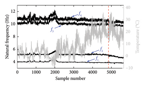
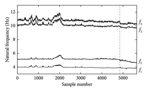
Using the stochastic subspace method, the long-term dynamic features of the Z24 bridge were identified in four modes [41]. Figure 14 illustrates the changes in air temperature and the identified natural frequency series over time, with the vertical dashed line indicating the onset of damage. Due to environmental variability, especially when the air temperature is below 0°C, the amplitude of frequency variations is significant, far exceeding the relative variation of frequencies during the damaged state. Such variability may induce erroneous damage detection, underscoring the necessity of removing environmental influences from the frequency data.

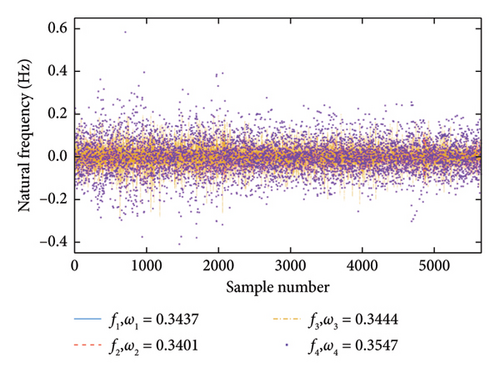
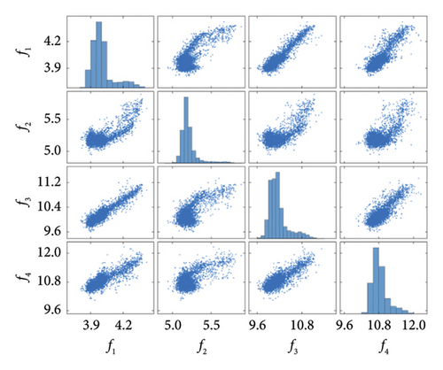
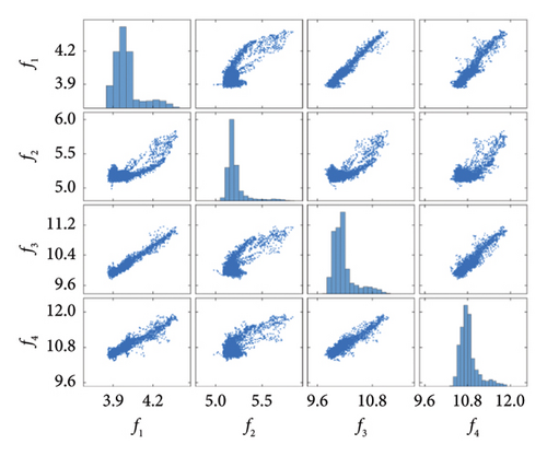
Before damage detection, the natural frequency time series is decomposed into two IMFs using VMD. Figure 15 shows the decomposed IMF results and their center frequencies. Note that the center frequency of the IMF1 signals here is also all zero, corresponding to nonstationary environmental influences. The average center frequencies of the IMF2 signals are approximately 0.346, corresponding to seasonal environmental influences. Therefore, the IMF2 signals were removed, and only IMF1 signals were utilized for damage detection. Figure 16 illustrates the distribution and mutual codistribution of the modal frequencies of the Z24 bridge both with (Figure 16(a)) and without (Figure 16(b)) the VMD method. Similar to the 7-DOF system in the numerical simulation, nonlinear relationships between the modal frequencies are observed, particularly the bilinear relationship between f₂ and other frequencies. In addition, the main diagonal entries indicate that the distribution of frequencies is non-Gaussian.

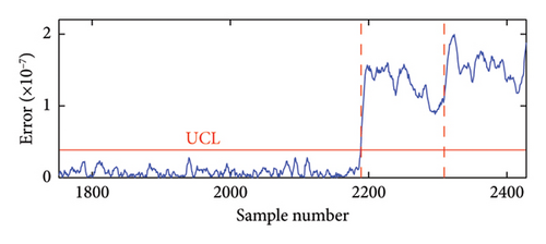
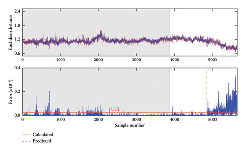
Following the damage detection procedure described in Section 3, the damage detection result obtained by the proposed method is shown in Figure 17. An enlarged view is provided to better illustrate the prediction error in the undamaged state. As observed from Figure 17, two important conclusions can be drawn. First, there are no sudden jumps or significant increases in prediction error in the undamaged state, particularly around the 2000th sample point. This indicates that the proposed method can effectively handle strong environmental variability. Second, since almost all prediction errors exceed the UCL line and there is a significant difference between the prediction errors of the damaged and undamaged states, it confirms that the proposed method not only accurately detects normal conditions but also has high damage detectability with almost no false alarms in the damaged state.

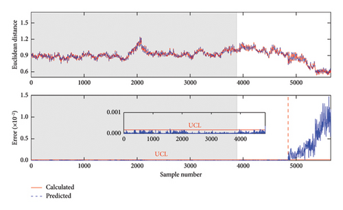
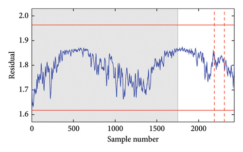
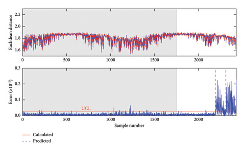
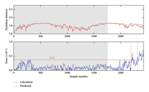
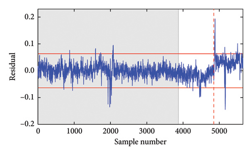
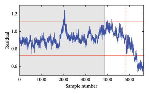
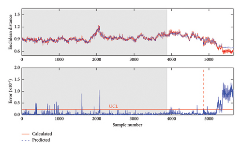
To further demonstrate the superiority of the proposed method, it is compared with VMD-cointegration, VMD–PCA, VMD–PCA–LSTM, and PCA–GPR methods similar to the preceding structure. The comparison results of these methods are shown in Figure 18, where the gray shading indicates the offline training phase. As the comparison between Figures 17 and 18 reveals, the proposed method achieves the best performance with the minimum false alarms. After that, the two methods, VMD–PCA–LSTM and PCA–GPR, outperformed VMD-cointegration and VMD–PCA. This is because the VMD–PCA–LSTM and PCA–GPR are nonlinear methods that can remove nonlinear environmental effects to a certain extent. However, due to the insufficient prediction accuracy of LSTM and the lack of noise removal using VMD, the damage detection results obtained by the two methods, VMD–PCA–LSTM and PCA–GPR, are still not accurate enough. Finally, the methods VMD-cointegration and VMD–PCA perform the worst in damage detectability. This suggests that due to the linear nature of the PCA and cointegration methods, they fail to remove the nonlinear environmental influences and accurately identify damage effectively.

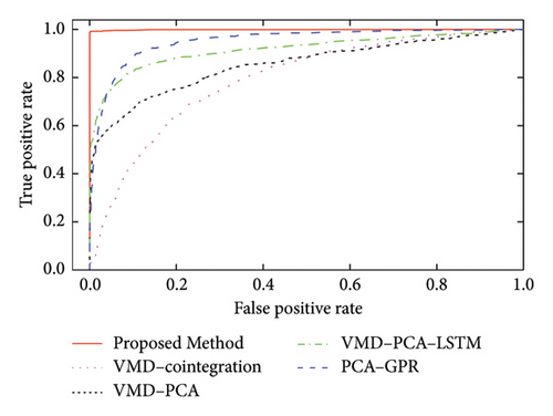
To compare the damage detection results of different methods in a single graph, the receiver operating characteristic (ROC) curve [68] widely used in machine learning, was introduced in this study. The ROC curve is a graphical representation, which is used to evaluate the performance of a binary classification model. It plots the TP rate (TPR) against the FPR at various threshold settings. In the context of SHM, “positive” and “negative” refer to the damaged and undamaged states, respectively. On the ROC curve, each point represents a TPR/FPR pair corresponding to a particular decision threshold. TPR is the ratio of correctly identified damage samples to all actual damage samples, while FPR is the ratio of incorrectly identified damage samples to all actual undamaged samples. The area under the roc curve (AUC) is a single scalar value summarizing the performance of the damage detection method. An AUC of 1 indicates perfect damage detection, while an AUC of 0.5 suggests no discriminative power (equivalent to random guessing). Therefore, a curve closer to the top-left corner indicates better performance, as it implies a higher TPR for a lower FPR; the diagonal line from (0, 0) to (1, 1) represents the performance of a random detection.

With these descriptions, Figure 19 shows the ROC curves of the proposed method and the VMD-cointegration, VMD–PCA, VMD–PCA–LSTM, and PCA–GPR methods. As can be observed, the best performance belongs to the proposed method. In contrast, the VMD-cointegration method has the worst damage detection performance, exhibits high FPR and low TPR across all thresholds, and has the smallest AUC. The main reason for this poor performance is the negative impact of nonlinear environmental effects, which cannot be effectively removed by the linear cointegration method. This conclusion also confirms the effectiveness of the proposed method in mitigating such nonlinear environmental effects.

7. Conclusion

In this paper, a nonlinear PCA method for structural damage detection under varying environmental conditions is proposed. The method employs VMD as a preprocessing algorithm, PCA to calculate the Euclidean distance of the reconstruction residual, and a GPR model to learn the underlying rules behind the calculation of the PCA Euclidean distance. Due to the linear nature of PCA, nonlinear EOV effects are retained in both the PCA Euclidean distance and its GPR–predicted values. By subtracting the GPR–predicted Euclidean distance from the PCA Euclidean distance, their common nonlinear environmental effects are eliminated. Consequently, the prediction error can be used as a damage feature insensitive to nonlinear EOVs.

The performance of the proposed method was first tested on a numerical example and further validated using long-term measurements of the Z24 bridge. The detailed conclusions are as follows:

1.
Despite the nonlinear environmental influences, the proposed VMD–PCA–GPR method clearly detected the occurrence of damage. The results indicate that the method has a high damage detectability even with a small number of frequency data and high data nonlinearity. However, the performance is affected by the size of the training dataset
2.
Comparative studies demonstrated that the proposed method outperforms several state-of-the-art techniques, such as PCA, cointegration, VMD–PCA–LSTM, and PCA–GPR methods. It was observed that VMD plays a crucial role in the success of the proposed method by effectively removing seasonal patterns and noise.

Conflicts of Interest

The authors declare no conflicts of interest.

Funding

This research work was jointly supported by the National Natural Science Foundation of China (Grant nos. 52078284 and 52308318), the Natural Science Foundation of Guangdong Province (Grant nos. 2023A1515012230 and 2021A1515011770), the Guangdong Province Special Fund for Science and Technology (“Big Project + Task List”) Project (Grant no. STKJ2023043), the STU Scientific Research Foundation for Talents (Grant nos. NTF18012 and NTF21019), the Anhui International Joint Research Center of Data Diagnosis and Smart maintenance on Bridge Structures (Grant no. 2022AHGHYB01), and the Open Fund for the State Key Laboratory of Coastal and Offshore Engineering (Grant no. LP2407).

Acknowledgments

This research work was jointly supported by the National Natural Science Foundation of China (Grant nos. 52078284 and 52308318), the Natural Science Foundation of Guangdong Province (Grant nos. 2023A1515012230 and 2021A1515011770), the Guangdong Province Special Fund for Science and Technology (“Big project + task list”) Project (Grant nos. STKJ2023043 and STKJ2024058), the STU Scientific Research Foundation for Talents (Grant nos. NTF18012 and NTF21019), the Anhui international joint research center of data diagnosis and smart maintenance on bridge structures (Grant no. 2022AHGHYB01), and the Open Fund for State Key Laboratory of Coastal and Offshore Engineering (Grant no. LP2407).

Open Research

Data Availability Statement

The research data will be available from the corresponding author upon reasonable request.

References

1 Zonzini F., Malatesta M. M., Bogomolov D., Testoni N., Marzani A., and De Marchi L., Vibration-Based SHM With Upscalable and Low-Cost Sensor Networks, IEEE Transactions on Instrumentation and Measurement. (2020) 69, no. 10, 7990–7998.
Web of Science® Google Scholar
2 Liu J. L., Wang S. F., Li Y. Z., and Yu A. H., Time-Varying Damage Detection in Beam Structures Using Variational Mode Decomposition and Continuous Wavelet Transform, Construction and Building Materials. (2024) 411, https://doi.org/10.1016/j.conbuildmat.2023.134416.
10.1016/j.conbuildmat.2023.134416
Web of Science® Google Scholar
3 Zhang H., Cheng X., Li Y., He D., and Du X., Rapid Seismic Damage State Assessment of RC Frames Using Machine Learning Methods, Journal of Building Engineering. (2023) 65, https://doi.org/10.1016/j.jobe.2022.105797.
10.1016/j.jobe.2022.105797
Web of Science® Google Scholar
4 Fan W. and Qiao P., Vibration-Based Damage Identification Methods: A Review and Comparative Study, Structural Health Monitoring. (2011) 10, no. 1, 83–111, https://doi.org/10.1177/1475921710365419, 2-s2.0-79751492551.
10.1177/1475921710365419
Web of Science® Google Scholar
5 Hou R. and Xia Y., Review on the New Development of Vibration-Based Damage Identification for Civil Engineering Structures: 2010–2019, Journal of Sound and Vibration. (2021) 491, https://doi.org/10.1016/j.jsv.2020.115741.
10.1016/j.jsv.2020.115741
Web of Science® Google Scholar
6 Avci O., Abdeljaber O., Kiranyaz S., Hussein M., Gabbouj M., and Inman D. J., A Review of Vibration-Based Damage Detection in Civil Structures: From Traditional Methods to Machine Learning and Deep Learning Applications, Mechanical Systems and Signal Processing. (2021) 147, https://doi.org/10.1016/j.ymssp.2020.107077.
10.1016/j.ymssp.2020.107077
Web of Science® Google Scholar
7 Ceravolo R., Coletta G., Miraglia G., and Palma F., Statistical Correlation Between Environmental Time Series and Data From Long-Term Monitoring of Buildings, Mechanical Systems and Signal Processing. (2021) 152, https://doi.org/10.1016/j.ymssp.2020.107460.
10.1016/j.ymssp.2020.107460
Web of Science® Google Scholar
8 Anastasopoulos D., Reynders E. P., Francois S. et al., Vibration-Based Monitoring of an FRP Footbridge With Embedded Fiber-Bragg Gratings: Influence of Temperature vs. Damage, Composite Structures. (2022) 287, https://doi.org/10.1016/j.compstruct.2022.115295.
10.1016/j.compstruct.2022.115295
Web of Science® Google Scholar
9 Xia Y., Hao H., Zanardo G., and Deeks A., Long Term Vibration Monitoring of an RC Slab: Temperature and Humidity Effect, Engineering Structures. (2006) 28, no. 3, 441–452, https://doi.org/10.1016/j.engstruct.2005.09.001, 2-s2.0-29244439612.
10.1016/j.engstruct.2005.09.001
Web of Science® Google Scholar
10 Li H., Li S., Ou J., and Li H., Modal Identification of Bridges Under Varying Environmental Conditions: Temperature and Wind Effects, Structural Control and Health Monitoring. (2010) 17, no. 5, 495–512.
10.1002/stc.319
Web of Science® Google Scholar
11 Zhang Y., Kurata M., and Lynch J. P., Long-term Modal Analysis of Wireless Structural Monitoring Data From a Suspension Bridge Under Varying Environmental and Operational Conditions: System Design and Automated Modal Analysis, Journal of Engineering Mechanics. (2017) 143, no. 4, https://doi.org/10.1061/(asce)em.1943-7889.0001198, 2-s2.0-85015938437.
10.1061/(ASCE)EM.1943-7889.0001198
Web of Science® Google Scholar
12 Teng J., Tang D. H., Hu W. H. et al., Mechanism of the Effect of Temperature on Frequency Based on Long-Term Monitoring of an Arch Bridge, Structural Health Monitoring. (2021) 20, no. 4, 1716–1737, https://doi.org/10.1177/1475921720931370.
10.1177/1475921720931370
Web of Science® Google Scholar
13 Peeters B., Maeck J., and Roeck G. D., Vibration-Based Damage Detection in Civil Engineering: Excitation Sources and Temperature Effects, Smart Materials and Structures. (2001) 10, no. 3, 518–527, https://doi.org/10.1088/0964-1726/10/3/314, 2-s2.0-0035360486.
10.1088/0964-1726/10/3/314
Web of Science® Google Scholar
14 Figueiredo E., Peres N., Moldovan I., and Nasr A., Impact of Climate Change on Long-Term Damage Detection for Structural Health Monitoring of Bridges, Structural Health Monitoring. (2024) https://doi.org/10.1177/14759217231224254.
10.1177/14759217231224254
Web of Science® Google Scholar
15 Wang Z., Yang D. H., Yi T. H., Zhang G. H., and Han J. G., Eliminating Environmental and Operational Effects on Structural Modal Frequency: A Comprehensive Review, Structural Control and Health Monitoring. (2022) 29, no. 11, https://doi.org/10.1002/stc.3073.
10.1002/stc.3073
PubMed Web of Science® Google Scholar
16 Soo Lon Wah W., Chen Y. T., and Owen J. S., A Regression-Based Damage Detection Method for Structures Subjected to Changing Environmental and Operational Conditions, Engineering Structures. (2021) 228, https://doi.org/10.1016/j.engstruct.2020.111462.
10.1016/j.engstruct.2020.111462
Google Scholar
17 Huang J. z., Yuan S. J., Li D. s., and Li H. n., A Kernel Canonical Correlation Analysis Approach for Removing Environmental and Operational Variations for Structural Damage Identification, Journal of Sound and Vibration. (2023) 548, https://doi.org/10.1016/j.jsv.2022.117516.
10.1016/j.jsv.2022.117516
Web of Science® Google Scholar
18 Maes K., Van Meerbeeck L., Reynders E. P. B., and Lombaert G., Validation of Vibration-Based Structural Health Monitoring on Retrofitted Railway Bridge KW51, Mechanical Systems and Signal Processing. (2022) 165, https://doi.org/10.1016/j.ymssp.2021.108380.
10.1016/j.ymssp.2021.108380
Web of Science® Google Scholar
19 Moser P. and Moaveni B., Environmental Effects on the Identified Natural Frequencies of the Dowling Hall Footbridge, Mechanical Systems and Signal Processing. (2011) 25, no. 7, 2336–2357, https://doi.org/10.1016/j.ymssp.2011.03.005, 2-s2.0-79960049610.
10.1016/j.ymssp.2011.03.005
Web of Science® Google Scholar
20 Peeters B. and De Roeck G., One-Year Monitoring of the Z24-Bridge: Environmental Effects Versus Damage Events, Earthquake Engineering & Structural Dynamics. (2001) 30, no. 2, 149–171.
10.1002/1096-9845(200102)30:2<149::AID-EQE1>3.0.CO;2-Z
Web of Science® Google Scholar
21 Zhang Y. M., Wang H., Bai Y., Mao J. X., Chang X. Y., and Wang L.-B., Switching Bayesian Dynamic Linear Model for Condition Assessment of Bridge Expansion Joints Using Structural Health Monitoring Data, Mechanical Systems and Signal Processing. (2021) 160, https://doi.org/10.1016/j.ymssp.2021.107879.
10.1016/j.ymssp.2021.107879
Web of Science® Google Scholar
22 Laory I., Trinh T. N., Smith I. F. C., and Brownjohn J. M. W., Methodologies for Predicting Natural Frequency Variation of a Suspension Bridge, Engineering Structures. (2014) 80, 211–221, https://doi.org/10.1016/j.engstruct.2014.09.001, 2-s2.0-84907746933.
10.1016/j.engstruct.2014.09.001
Web of Science® Google Scholar
23 Han Q., Ma Q., Dang D., and Xu J., Modal Parameters Prediction and Damage Detection of Space Grid Structure Under Environmental Effects Using Stacked Ensemble Learning, Structural Control and Health Monitoring. (2023) 2023, no. 1, 1–24, https://doi.org/10.1155/2023/5687265.
10.1155/2023/5687265
Web of Science® Google Scholar
24 Worden K. and Cross E., On Switching Response Surface Models, With Applications to the Structural Health Monitoring of Bridges, Mechanical Systems and Signal Processing. (2018) 98, 139–156, https://doi.org/10.1016/j.ymssp.2017.04.022, 2-s2.0-85022219703.
10.1016/j.ymssp.2017.04.022
Web of Science® Google Scholar
25 Ni Y. Q., Zhou H. F., and Ko J. M., Generalization Capability of Neural Network Models for Temperature-Frequency Correlation Using Monitoring Data, Journal of Structural Engineering. (2009) 135, no. 10, 1290–1300, https://doi.org/10.1061/(asce)st.1943-541x.0000050, 2-s2.0-70349336497.
10.1061/(ASCE)ST.1943-541X.0000050
Web of Science® Google Scholar
26 Abbassi A., Römgens N., Tritschel F. F., Penner N., and Rolfes R., Evaluation of Machine Learning Techniques for Structural Health Monitoring Using Ultrasonic Guided Waves Under Varying Temperature Conditions, Structural Health Monitoring. (2023) 22, no. 2, 1308–1325, https://doi.org/10.1177/14759217221107566.
10.1177/14759217221107566
Web of Science® Google Scholar
27 Yan A. M., Kerschen G., De Boe P., and Golinval J. C., Structural Damage Diagnosis Under Varying Environmental Conditions—Part I: A Linear Analysis, Mechanical Systems and Signal Processing. (2005) 19, no. 4, 847–864, https://doi.org/10.1016/j.ymssp.2004.12.002, 2-s2.0-17644426027.
10.1016/j.ymssp.2004.12.002
Web of Science® Google Scholar
28 Dao P. B. and Staszewski W. J., Cointegration and How it Works for Structural Health Monitoring, Measurement. (2023) 209, https://doi.org/10.1016/j.measurement.2023.112503.
10.1016/j.measurement.2023.112503
Web of Science® Google Scholar
29 Hassani S., Mousavi M., and Dackermann U., Johansen Cointegration of Frequency Response Functions Contaminated With Nonstationary Colored Noise for Structural Damage Detection, Journal of Sound and Vibration. (2023) 552, https://doi.org/10.1016/j.jsv.2023.117641.
10.1016/j.jsv.2023.117641
Web of Science® Google Scholar
30 Wang X., Li L., Beck J. L., and Xia Y., Sparse Bayesian Factor Analysis for Structural Damage Detection Under Unknown Environmental Conditions, Mechanical Systems and Signal Processing. (2021) 154, https://doi.org/10.1016/j.ymssp.2020.107563.
10.1016/j.ymssp.2020.107563
Web of Science® Google Scholar
31 Rainieri C., Magalhaes F., Gargaro D., Fabbrocino G., and Cunha A., Predicting the Variability of Natural Frequencies and Its Causes by Second-Order Blind Identification, Structural Health Monitoring. (2019) 18, no. 2, 486–507, https://doi.org/10.1177/1475921718758629, 2-s2.0-85042523420.
10.1177/1475921718758629
Web of Science® Google Scholar
32 Diao Y., Sui Z., and Guo K., Structural Damage Identification Under Variable Environmental/Operational Conditions Based on Singular Spectrum Analysis and Statistical Control Chart, Structural Control and Health Monitoring. (2021) 28, no. 6, https://doi.org/10.1002/stc.2721.
10.1002/stc.2721
PubMed Web of Science® Google Scholar
33 Kullaa J., Eliminating Environmental or Operational Influences in Structural Health Monitoring Using the Missing Data Analysis, Journal of Intelligent Material Systems and Structures. (2009) 20, no. 11, 1381–1390, https://doi.org/10.1177/1045389x08096050, 2-s2.0-67650246038.
10.1177/1045389X08096050
Web of Science® Google Scholar
34 Liu A., Wang L. Z., Bornn L., and Farrar C., Robust Structural Health Monitoring Under Environmental and Operational Uncertainty With Switching State-Space Autoregressive Models, Structural Health Monitoring. (2019) 18, no. 2, 435–453, https://doi.org/10.1177/1475921718757721, 2-s2.0-85061002152.
10.1177/1475921718757721
Web of Science® Google Scholar
35 Hsu T. Y. and Loh C. H., Damage Detection Accommodating Nonlinear Environmental Effects by Nonlinear Principal Component Analysis, Structural Control and Health Monitoring: The Official Journal of the International Association for Structural Control and Monitoring and of the European Association for the Control of Structures. (2010) 17, no. 3, 338–354.
10.1002/stc.320
Google Scholar
36 Yang C. and Liu Y., Detecting the Damage of Bridges Under Changing Environmental Conditions Using the Characteristics of the Nonlinear Narrow Dimension of Damage Features, Mechanical Systems and Signal Processing. (2021) 159, https://doi.org/10.1016/j.ymssp.2021.107842.
10.1016/j.ymssp.2021.107842
Web of Science® Google Scholar
37 Prawin J. and Bhaskara G. V., Outlier Analysis Combined With Gaussian Mixture Model for Structural Damage Detection, Materials Today: Proceedings. (2023) .
10.1016/j.matpr.2023.03.533
Google Scholar
38 Peng Z., Li J., and Hao H., Structural Damage Detection via Phase Space Based Manifold Learning Under Changing Environmental and Operational Conditions, Engineering Structures. (2022) 263, https://doi.org/10.1016/j.engstruct.2022.114420.
10.1016/j.engstruct.2022.114420
Web of Science® Google Scholar
39 Shi H., Worden K., and Cross E. J., A Regime-Switching Cointegration Approach for Removing Environmental and Operational Variations in Structural Health Monitoring, Mechanical Systems and Signal Processing. (2018) 103, 381–397, https://doi.org/10.1016/j.ymssp.2017.10.013, 2-s2.0-85033605702.
10.1016/j.ymssp.2017.10.013
Web of Science® Google Scholar
40 Huang J. z., Li D. s., and Li H. n., A New Regime-Switching Cointegration Method for Structural Health Monitoring Under Changing Environmental and Operational Conditions, Measurement. (2023) 212, https://doi.org/10.1016/j.measurement.2023.112682.
10.1016/j.measurement.2023.112682
Web of Science® Google Scholar
41 Huang J. z., Liu Y. J., Qi H., Chen S. X., and Li D. s., A Novel Nonlinear ICA Method for Structural Health Monitoring Under Nonlinear Environmental or Operational Influences, Structures. (2025) 71, https://doi.org/10.1016/j.istruc.2024.108118.
10.1016/j.istruc.2024.108118
Web of Science® Google Scholar
42 Sarmadi H., Entezami A., and De Michele C., Probabilistic Data Self-Clustering Based on Semi-Parametric Extreme Value Theory for Structural Health Monitoring, Mechanical Systems and Signal Processing. (2023) 187, https://doi.org/10.1016/j.ymssp.2022.109976.
10.1016/j.ymssp.2022.109976
Web of Science® Google Scholar
43 Entezami A., Sarmadi H., and Behkamal B., Short-Term Damage Alarming With Limited Vibration Data in Bridge Structures: A Fully Non-Parametric Machine Learning Technique, Measurement. (2024) 235, https://doi.org/10.1016/j.measurement.2024.114935.
10.1016/j.measurement.2024.114935
Web of Science® Google Scholar
44 Mousavi M. and Gandomi A. H., Prediction Error of Johansen Cointegration Residuals for Structural Health Monitoring, Mechanical Systems and Signal Processing. (2021) 160, https://doi.org/10.1016/j.ymssp.2021.107847.
10.1016/j.ymssp.2021.107847
Web of Science® Google Scholar
45 Daneshvar M. H., Sarmadi H., and Yuen K. V., A Locally Unsupervised Hybrid Learning Method for Removing Environmental Effects Under Different Measurement Periods, Measurement. (2023) 208, https://doi.org/10.1016/j.measurement.2023.112465.
10.1016/j.measurement.2023.112465
Web of Science® Google Scholar
46 Sarwar M. Z. and Cantero D., Probabilistic Autoencoder-Based Bridge Damage Assessment Using Train-Induced Responses, Mechanical Systems and Signal Processing. (2024) 208, https://doi.org/10.1016/j.ymssp.2023.111046.
10.1016/j.ymssp.2023.111046
Web of Science® Google Scholar
47 Diord S., Magalhães F., Cunha Á., Caetano E., and Martins N., Automated Modal Tracking in a Football Stadium Suspension Roof for Detection of Structural Changes, Structural Control and Health Monitoring. (2017) 24, no. 11, https://doi.org/10.1002/stc.2006, 2-s2.0-85030703204.
10.1002/stc.2006
Web of Science® Google Scholar
48 Hu W.-H., Thöns S., Rohrmann R. G., Said S., and Rücker W., Vibration-Based Structural Health Monitoring of a Wind Turbine System. Part I: Resonance Phenomenon, Engineering Structures. (2015) 89, 260–272, https://doi.org/10.1016/j.engstruct.2014.12.034, 2-s2.0-84925218032.
10.1016/j.engstruct.2014.12.034
Web of Science® Google Scholar
49 Lakshmi K. and Rama Mohan Rao A., A Robust Damage-Detection Technique With Environmental Variability Combining Time-Series Models With Principal Components, Nondestructive Testing and Evaluation. (2014) 29, no. 4, 357–376, https://doi.org/10.1080/10589759.2014.949709, 2-s2.0-84907590299.
10.1080/10589759.2014.949709
Web of Science® Google Scholar
50 Mario Azzara R., De Roeck G., Girardi M., Padovani C., Pellegrini D., and Reynders E., The Influence of Environmental Parameters on the Dynamic Behaviour of the San Frediano Bell Tower in Lucca, Engineering Structures. (2018) 156, 175–187, https://doi.org/10.1016/j.engstruct.2017.10.045, 2-s2.0-85034237211.
10.1016/j.engstruct.2017.10.045
Web of Science® Google Scholar
51 Jin S. S., Cho S., and Jung H. J., Adaptive Reference Updating for Vibration-Based Structural Health Monitoring Under Varying Environmental Conditions, Computers & Structures. (2015) 158, 211–224, https://doi.org/10.1016/j.compstruc.2015.06.001, 2-s2.0-84933505124.
10.1016/j.compstruc.2015.06.001
Web of Science® Google Scholar
52 Xu M., Li J., Wang S., Hao H., Tian H., and Han J., Structural Damage Detection by Integrating Robust PCA and Classical PCA for Handling Environmental Variations and Imperfect Measurement Data, Advances in Structural Engineering. (2022) 25, no. 8, 1815–1828, https://doi.org/10.1177/13694332221079090.
10.1177/13694332221079090
Web of Science® Google Scholar
53 Ma Z., Yun C. B., Wan H. P., Shen Y., Yu F., and Luo Y., Probabilistic Principal Component Analysis-Based Anomaly Detection for Structures With Missing Data, Structural Control and Health Monitoring. (2021) 28, no. 5, https://doi.org/10.1002/stc.2698.
10.1002/stc.2698
PubMed Web of Science® Google Scholar
54 Fernandez-Navamuel A., Magalhães F., Zamora-Sánchez D., Omella Á. J., Garcia-Sanchez D., and Pardo D., Deep Learning Enhanced Principal Component Analysis for Structural Health Monitoring, Structural Health Monitoring. (2022) 21, no. 4, 1710–1722, https://doi.org/10.1177/14759217211041684.
10.1177/14759217211041684
Web of Science® Google Scholar
55 Yan A. M., Kerschen G., De Boe P., and Golinval J. C., Structural Damage Diagnosis Under Varying Environmental Conditions—Part II: Local PCA for Non-Linear Cases, Mechanical Systems and Signal Processing. (2005) 19, no. 4, 865–880, https://doi.org/10.1016/j.ymssp.2004.12.003, 2-s2.0-17644400142.
10.1016/j.ymssp.2004.12.003
Web of Science® Google Scholar
56 Zang J. G., Huang H. B., Sun Z. G., and Wang D.-S., Subdomain Principal Component Analysis for Damage Detection of Structures Subjected to Changing Environments, Engineering Structures. (2023) 288, https://doi.org/10.1016/j.engstruct.2023.116265.
10.1016/j.engstruct.2023.116265
Web of Science® Google Scholar
57 Santos A., Figueiredo E., Silva M., Sales C., and Costa J., Machine Learning Algorithms for Damage Detection: Kernel-Based Approaches, Journal of Sound and Vibration. (2016) 363, 584–599, https://doi.org/10.1016/j.jsv.2015.11.008, 2-s2.0-84949908086.
10.1016/j.jsv.2015.11.008
Web of Science® Google Scholar
58 Bro R. and Smilde A. K., Principal Component Analysis, Analytical Methods. (2014) 6, no. 9, 2812–2831, https://doi.org/10.1039/c3ay41907j, 2-s2.0-84898639050.
10.1039/C3AY41907J
CAS Web of Science® Google Scholar
59 Wang S., Wang H., Xu M., and Guo J., Identifying the Presence of Structural Damage: A Statistical Hypothesis Testing Approach Combined With Residual Strain Energy, Mechanical Systems and Signal Processing. (2020) 140, https://doi.org/10.1016/j.ymssp.2020.106655.
10.1016/j.ymssp.2020.106655
Web of Science® Google Scholar
60 Schulz E., Speekenbrink M., and Krause A., A Tutorial on Gaussian Process Regression: Modelling, Exploring, and Exploiting Functions, Journal of Mathematical Psychology. (2018) 85, 1–16, https://doi.org/10.1016/j.jmp.2018.03.001, 2-s2.0-85047623441.
10.1016/j.jmp.2018.03.001
Web of Science® Google Scholar
61 Dragomiretskiy K. and Zosso D., Variational Mode Decomposition, IEEE Transactions on Signal Processing. (2014) 62, no. 3, 531–544, https://doi.org/10.1109/tsp.2013.2288675, 2-s2.0-84893418756.
10.1109/TSP.2013.2288675
Web of Science® Google Scholar
62 Shi H. C., Worden K., and Cross E. J., A Cointegration Approach for Heteroscedastic Data Based on a Time Series Decomposition: An Application to Structural Health Monitoring, Mechanical Systems and Signal Processing. (2019) 120, 16–31, https://doi.org/10.1016/j.ymssp.2018.09.036, 2-s2.0-85055196354.
10.1016/j.ymssp.2018.09.036
Web of Science® Google Scholar
63 Hu W. H., Cunha Á., Caetano E., Rohrmann R. G., Said S., and Teng J., Comparison of Different Statistical Approaches for Removing Environmental/Operational Effects for Massive Data Continuously Collected From Footbridges, Structural Control and Health Monitoring. (2017) 24, no. 8, https://doi.org/10.1002/stc.1955, 2-s2.0-84991809185.
10.1002/stc.1955
Web of Science® Google Scholar
64 Das S. and Saha P., Performance of Hybrid Decomposition Algorithm Under Heavy Noise Condition for Health Monitoring of Structure, Journal of Civil Structural Health Monitoring. (2020) 10, no. 4, 679–692, https://doi.org/10.1007/s13349-020-00412-5.
10.1007/s13349-020-00412-5
Web of Science® Google Scholar
65 Bagheri A., Ozbulut O. E., and Harris D. K., Structural System Identification Based on Variational Mode Decomposition, Journal of Sound and Vibration. (2018) 417, 182–197, https://doi.org/10.1016/j.jsv.2017.12.014, 2-s2.0-85041500200.
10.1016/j.jsv.2017.12.014
Web of Science® Google Scholar
66 Lv Z., Tang B., Zhou Y., and Zhou C., A Novel Method for Mechanical Fault Diagnosis Based on Variational Mode Decomposition and Multikernel Support Vector Machine, Shock and Vibration. (2016) 2016, no. 1, 1–11, https://doi.org/10.1155/2016/3196465, 2-s2.0-84955509365.
10.1155/2016/3196465
Web of Science® Google Scholar
67 Sousa Tomé E., Pimentel M., and Figueiras J., Damage Detection Under Environmental and Operational Effects Using Cointegration Analysis-Application to Experimental Data From a Cable-Stayed Bridge, Mechanical Systems and Signal Processing. (2020) 135, https://doi.org/10.1016/j.ymssp.2019.106386.
10.1016/j.ymssp.2019.106386
Google Scholar
68 Figueiredo E., Park G., Farrar C. R., Worden K., and Figueiras J., Machine Learning Algorithms for Damage Detection Under Operational and Environmental Variability, Structural Health Monitoring. (2010) 10, no. 6, 559–572, https://doi.org/10.1177/1475921710388971, 2-s2.0-80455123889.
10.1177/1475921710388971
Web of Science® Google Scholar

All articles

A Novel Nonlinear Output-Only Damage Detection Method Based on the Prediction Error of PCA Euclidean Distances Under Environmental and Operational Variations

Abstract

1. Introduction

2. Contributions

3. PCA