Robust Damage Detection and Localization Under Varying Environmental Conditions Using Neural Networks and Input-Residual Correlations
Abstract
This study aims to evaluate sequences of raw time series using an autoencoder structure for unsupervised damage detection and localization under varying environmental conditions (ECs). When it comes to structural health monitoring (SHM) for real-world applications, data-driven models need to improve sensitivity and robustness toward damage due to the EC-dependent variance. For systems situated outdoors, changing ECs affects the stiffness properties without causing permanent alterations to the structure. Applying data normalization strategies to consider these natural variations is not easy to conduct and is unfavorable for sensitivity regarding damage. To address these challenges, the model’s input variables are non-standardized to avoid input-related modifications and to feature a higher sensitivity toward structural changes. The autoencoder’s ability to capture structural variations caused by ECs and to handle non-standardized time series data makes it favorable for real-world applications. By quantifying the input-residual correlations, sensitivity, and robustness can be improved; no adjustments to the model have to be made. The autoencoder’s black-box nature is inspected by analyzing a linear dynamic 8DOF system and the Leibniz University Structure for Monitoring (LUMO). The neural network’s structure is identified by tracking the residual correlation. Here, a common test statistic of a whiteness test is used to find an optimal choice of the bottleneck dimension. Significantly increased robustness and sensitivity toward damage when evaluating the input-residual correlations instead of the reconstruction error is observed. To capture the temperature-dependent structural response for experimental validation, 10-min data sets of different structural temperatures are given to the neural network during training. It was derived that for damage detection, an amplitude-related normalization is inevitable due to the different excitation intensities in real life, which was carried out using input-residual correlations quantified by a Pearson coefficient. Considering the results obtained, autoencoders with non-standardized time series and input-residual correlations demonstrate a potent tool for vibration-based damage identification.
1. Introduction
Recent events such as earthquakes [1] or failure of bridges [2, 3] have shown that constructions often do not correspond to the target conditions. Due to the constant increase in building sizes and the challenges of sustainability and efficiency, there are higher demands on engineers to ensure structural health while also considering changes in the material integrity or faulty construction processes that need to be observed [4]. Although it is often impossible to avoid building defects or construction faults, it is nevertheless important to be able to monitor them reliably as part of structural health monitoring (SHM). Observing and analyzing engineering structures over time and using periodically sampled vibration signals to monitor anomalies is classically referred to as vibration-based SHM. It is conventional to define the goals according to the five levels of the SHM to subsequently (i) detect, (ii) localize, (iii) classify, and (iv) quantify damage, as well as to (v) predict the remaining lifetime of the structure [5, 6]. In vibration-based SHM, it comes naturally to track modal parameters because damage alters the dynamic properties of the system [7] and modal parameters can be easily interpreted. The identification of the modal parameters can reliably reveal structural changes [8] and, given a dense sensor network, also provides information on the location of the damage [9, 10]. However, there is a prevailing opinion that these measures often lack sensitivity in detecting minor damages [11]. Additionally, almost all vibrating structures subject to monitoring undergo varying environmental and operational conditions (EOCs), which affect the structure’s response and its modal properties. Therefore, the detection and localization of structural damage under changing EOCs is an essential issue in the SHM research community [12].
In SHM, the models utilized can be divided by whether physical knowledge is incorporated into them. Physics-based models constitute scientific principles, whereas data-driven models strictly rely on measurements [11]. In model-based SHM, the results are limited by the accuracy of the underlying models, which may be challenging to develop for complex structures or in varying environmental conditions. In contrast, the dependence on the quality and representativeness of training data is crucial for data-driven models, and the “black-box” nature of some machine learning algorithms needs to be regarded. The latter is focused in this work to tackle the problem of damage detection and localization under varying environmental conditions in output-only vibration-based SHM. It is expected that alternations in structural systems significantly influence the estimated values derived from the trained model, and the evaluation of the model’s residuals enables damage identification.
The task of damage detection in unsupervised data-driven vibration-based SHM has been addressed by several works. In SHM, the term unsupervised specifies that information on the damaged state is not used during training [6]. Supervised methods that require labeled training data from both healthy and various damaged states of the monitored structure are generally impractical for civil infrastructure. This is due to the rarity, cost, and generally limited accessibility of data representing different damage states in these structures [13]. It is worth mentioning here that physics-based models can reach the highest levels of SHM in unsupervised vibration-based SHM. It has been clarified in [6] that the task of unsupervised damage localization represents the highest level to be achieved in data-driven SHM as the realization of higher levels needs prior insights. In data-driven SHM, deep learning approaches have generally gained much attention in the last decade due to their ability to process a lot of information simultaneously. An overview of various advanced deep learning operations and networks is given in [14]. A vision-based method by Cha et al. [15] enabled to substantiate the existence of cracks by utilizing a convolutional neural network automatically abstracting the image’s patterns. In [16], raw acceleration signals were first processed using the synchrosqueezed wavelet transform and fast Fourier transform, and features were subsequently extracted by a deep restricted Boltzmann machine from two sets of preprocessed signals: one representing the healthy state of a small-scale reinforced concrete building and the other corresponding to the unknown health conditions. The novel approach allows for assessing the global and local conditions. Silva et al. [17] suggested enhancing the extraction of critical structural patterns by employing a deep principal component analysis (PCA) framework. The methodology was implemented on a prestressed concrete bridge with increasing damage and a three-segment suspension bridge, both exposed to varying conditions due to environmental factors. In another interesting work, Hsu et al. [18] were able to continuously track the health conditions of the Sayano-Shushenskaya Dam under external factors influencing the system’s dynamics. With minimal alterations to the natural frequencies, the simulated crack remained challenging to accurately detect, implying the necessity for higher sensitivity toward damage. By employing a deep autoencoder combined with a one-class support vector machine to identify structural changes consistently, the authors in [19] investigated its functionality on a laboratory steel bridge and also on a 12-story numerical building model showcasing impressive performance abilities. Another interesting approach from the same authors involves exploring several machine learning methods and a deep autoencoder to monitor the changes correlated to the local weakening of a bridge [20].
Due to the increasing quality of sensor equipment and data acquisition systems, for vibration-based damage localization, the use of models relying solely on measurement data has increased in recent years. Anaissi et al. [21] used the frequency domain of standardized time series data as the inputs of a variational autoencoder to monitor the health state of two bridges and a three-story building. By advancing a clustering strategy, Cha et al. [13] presented detection and localization capabilities on a scaled-down steel model subjected to several damage scenarios. Ma et al. [22] acquired accelerometer signals to implicitly extract meaningful features employing a convolutional–variational autoencoder for persistent bridge monitoring. A similar work investigated the same model type to monitor a subway tunnel using wavelet packet energy [23]. Wernitz [11] addressed the problem of vibration-based monitoring under varying EOCs by implementing effective parametric autocovariance least-squares using Kalman filter-based damage localization. However, the effectiveness of accounting for varying external factors remains to be empirically validated, and further improvements for stable data normalization are needed. Römgens et al. [24] introduced an autoencoder-based approach for damage localization under slightly fluctuating EOCs. A pre-classified part of the measurement campaign was analyzed in order to demonstrate the basic application of the methodology. Further, the approach did not address damage detection using autoencoders with short-term sequences. This introduces the need for data normalization techniques as the excitation levels vary and temperature effects play a crucial role. The bottleneck dimensioning has been identified as the most important parameter of the hypertuning, which was simplified by approximation of the reconstruction error in frequency space. The underlying work builds on these aspects and investigates long-term analysis [25]. In general, two primary observations from the literature drive the present work. First, despite the literature review in the context of vibration-based SHM, to the best of our knowledge, there is still no purely data-driven method to reliably detect and localize damage under varying excitation intensities and temperature conditions in real-life validation. Most proposed methods lack robustness and sensitivity toward damage and struggle to properly account for the EOC-dependent variance. Second, several works [16, 19, 22, 23] limit their investigation to laboratory experiments (or numerical simulations), which involves keeping certain factors constant to not only isolate the effect of the variable under investigation but also reduce their applicability. In this work, the sensitivity of the method regarding real-life validation is given priority; therefore, no data preprocessing of the raw signals is applied. A neural network, which can handle the non-standardized inputs, is used. The structural variations caused by EOCs are captured by exploiting the autoencoder’s ability to learn different states and tested in a real-life validation case. Further, the input-residual correlations are evaluated to significantly improve sensitivity and robustness without adjusting the model. Additionally, a well-performing architecture can be found by automating the design process.
The contribution of this paper is fourfold: (i) The autoencoder’s inputs are non-standardized time series to be adopted for the task of robust damage detection and localization across diverse environmental conditions. (ii) In principle, training the autoencoder is the most time-consuming task of the methodology. To reduce computational costs during the neural architecture search, the smallest layer of the neural network (further referred to as bottleneck dimension or latent space) is determined by evaluating the PCA. It is shown that the common test statistics of whiteness property can narrow down the optimal-performing model to avoid under and over-fitting depending on the number of principal components. (iii) Significant improvement in damage detection performance is demonstrated by evaluating input-residual correlations of the autoencoder instead of the commonly used error metric. Amplitude-related normalization is provided by quantifying the correlations using Pearson correlation coefficients. (iv) We validate our method on an open-access benchmark to facilitate comparison to other methods. We also provide an overview of existing results obtained using data-driven approaches regarding Leibniz University Structure for Monitoring (LUMO).
This paper consists of five sections. The section on theoretical background gives a detailed description of the mathematical model to detect and localize potential structural damage using input-residual correlations. Following this, acceleration time series with different amplitudes are extracted from simulated measurements to derive a robust damage detection technique and localize the damage using the same model’s residuals. Experimental studies are further introduced in the next section, and herein considered varying environmental conditions are analyzed using the proposed neural network framework, which is then compared to existing contributions. The last section gives a summary and an outlook.
2. Theoretical Background
The autoencoder-based strategy leverages non-preprocessed sequences of time series data. The autoencoder’s process and structure are briefly described to give the reader an understanding of the basic approach. The detection of structural change can be carried out using the commonly employed reconstruction error of the model [26]. The innovative input-residual correlations quantified by a Pearson correlation coefficient are presented to improve the performance of the evaluation. The damage localization approach also consists of evaluating the residuals of the autoencoder under the consideration of the neural network’s inputs, which has been introduced in [27]. Lastly, the training process examined is described in detail, i.e., how the dimensioning of the autoencoder needs to be carried out.
2.1. Autoencoder
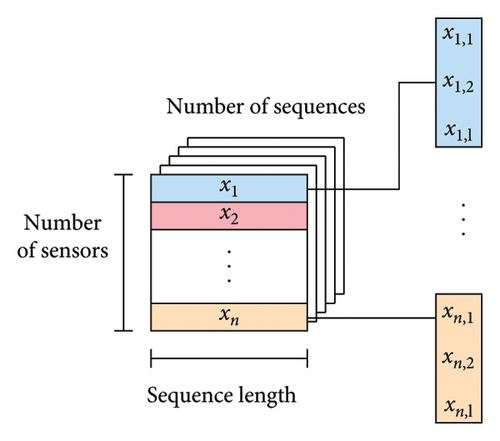
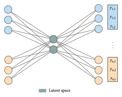
As illustrated in Figure 1, the basic idea is to extract features from the time sequences by reducing their dimension [27]. At its core, an autoencoder learns to create a lower-dimensional feature representation from the input data. This process begins by encoding the high-dimensional input data x[n × l], where n represents the number of sensors and l denotes the sequence length, into a lower-dimensional latent space d (with n × l > d). The encoded representation is then decoded back into the original input space [n × l], to reconstruct the input data, namely, the target data y as accurately as possible.
2.2. Residual Pearson Correlation for Damage Detection
Note that the error metric is very similar to the previously introduced neural network’s loss function in equation (2). The reconstruction error—in the given case defined as the MAE—can be used as an anomaly score because it is typically low when the model is well trained and the input data fit the model architecture. However, when the model encounters data that do not conform to the patterns it learned during training, the model struggles to accurately reconstruct the unknown signal characteristics. This process produces a sensitive indicator for structural anomalies based on shifts in residual behavior.
The covariances of the model’s inputs xi and the residuals er (cf. equation (5)) are divided by the product of their standard deviations (, ). The linear correlations of an input time series to each residual time series are calculated with the covariance to quantify the remaining relationship. It is assumed that due to the model’s structure information not mapped by the model is distributed over the residual terms of the outputs. If the model encounters data that do not match the patterns it has learned during training, the residual time series consists heavily of deterministic parts from the input signals. As a result, there is a high correlation between the inputs and the residuals of the model. In contrast, a well-trained model absorbs most of the input data when evaluating the same health state and, in consequence, the errors mostly consist of noise highly uncorrelated to any input signals. In this work, further metrics such as the evaluation of the bottleneck dimension [31] or using the Mahalanobis distance [32] instead of the MAE have been investigated but were not found to be applicable. The application of the original-to-reconstructed-signal ratio [19] has been particularly interesting as it features amplitude-related normalization. However, to highlight the effects of different excitation intensities and to compare the improvement driven by the input-residual consideration, the results obtained utilizing the MAE are presented.
2.3. Residual Covariance for Damage Localization
Notably, equations (7) and (8) are very similar. In equation (8), the amplitude-related normalization utilizing the product of standard deviations is not performed. In data-driven SHM, for damage localization, the position of damage is derived by comparing the anomaly scores of individual sensors, such that the highest outputs correspond to the location of structural degradation [11]. Thus, the absolute values of the damage index analyzing different channels within a given period do not affect the outcomes of the damage localization, as a relative measure is decisive.
The idea is to use the autoencoder to filter the most relevant information for the healthy state, leaving estimation errors consisting mainly of stochastic components highly uncorrelated to any input signal. When structural damage occurs, correlations quantified by the residual covariances increase locally, enabling localization. Autoencoders are advantageous due to their structure, which leads to (measurement) noise being distributed equally to the outputs of the model, giving an excellent baseline for robust damage localization [27].
2.4. Dimensioning of the Autoencoder
The whiteness test essentially detects residual correlations of the individual sequences. Small values for the estimated serial correlation in the case of discrete time (autocorrelation) mean that the model effectively captures the most important information. For a low number of principal components, there are strong linear dependencies within the time series error, which are quantified by the test statistics. Increasing the number of principal components improves the performance of the model up to the maximal uncorrelatedness of estimation errors. Crucially, the independence of estimation errors quantified by the test statistic reflects the worsening of the model when for a high number of principal components noise or random fluctuations in the data are learned. This non-conventional approach is mainly driven by the non-standardized inputs of the model. However, the autocorrelation approach is particularly valuable when dealing with time series.
To account for temperature-dependent varying states of the structure, the autoencoder’s ability to capture variabilities in its learned representation is utilized. To effectively train an autoencoder for different temperature conditions, the training phase is diversified by selecting data sets including various temperature states.
The proposed method defines boundaries for the neural network architecture by specifying its input dimension and information compression. Bayesian techniques enable effective configuration search completion. Notable, the training procedure has been focused on long training with varying learning rates to optimize the weights to the maximum. This reduces the dependency on the cost function used during training and the initial learning rate.
3. Simulation Studies
Simulation studies allow conclusions to be drawn about method development, independent of external influences such as field experiments. In particular, they can be used to improve the model’s performance and enable easy comparability with other methods. The 8DOF simulation model used in the given paper is first described, and the neural architecture search of the autoencoder is conducted. The benefits of input-residual correlations for damage detection regarding changing excitation intensities are demonstrated in the following. This research also addresses complex failure scenarios characterized by the coupled behavior of several interacting system parameters.
3.1. 8DOF System

| Name | Noise level (SNR) (dB) | Pos. | f1 (Hz) | f2 (Hz) | f3 (Hz) | f4 (Hz) |
|---|---|---|---|---|---|---|
| Healthy | 50 | — | 5.50 | 10.89 | 15.91 | 20.47 |
| Damaged | 50 | k1, k6 | 5.46 | 10.71 | 15.64 | 20.33 |
- Note: The signal-to-noise-ratio (SNR) is expressed to quantify the precision of the simulated signals.
In the present example, the test statistics for the whiteness property given in equation 10 can be effectively applied to find an optimal-performing architecture for the neural network. Low linear dependencies between estimation errors in the range of 100–150 principal components can be specially observed as shown in Figure 3. For the dimensioning of the autoencoder, a bottleneck dimension of 121 is determined based on the results obtained, as there is no large scatter in the test statistics of different channels. For a low number of principal components, the error terms still show significant linear dependencies demonstrated by the whiteness test statistics. This indicates that the model struggles to reconstruct the input data or abstract the most important dynamic properties due to an insufficient number of parameters and an underfitting of the model. Regarding 200 or more principal components, the test statistics for whiteness increase for a higher number of principal components, an overfitting of the model. The results are particularly appealing due to two observations. Firstly, there is a pronounced minimum of the test statistic, making it easy to derive an optimal model. Secondly, this minimum exists without introducing a penalty function regarding the model order.
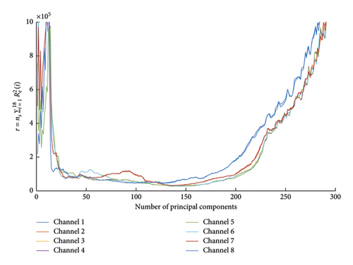
The course is not tracked as an average value over the number of principal components to recognize the effects of individual reconstructed signals. For example, the mean value for 90 principal components is relatively small, but the performance of channel 7 differs significantly from the other channels, indicating an underfitting of the model.
The number of inputs (320) is defined by the number of signals multiplied by the estimated sequence length determined earlier. Further, the latent representation (121) reveals the model’s degree of information compression. Subject to the boundary conditions, which in the given scenario are the input and bottleneck dimension of the dimension reduction model, the other parameters such as the learning rate and the number of neurons in the encoder and decoder can be optimized concerning the validation error’s performance. The batch size is consistently defined as 256, and early stopping is applied to prevent overfitting and improve generalization performance.
3.2. Damage Detection
In principle, it is natural to use the reconstruction error of the autoencoder as a damage-sensitive feature, i.e., to accumulate the absolute mean values of the residuals. However, when comparing time series with different vibration amplitudes, the damage-sensitive features require adaptation to eliminate the effects of fluctuating excitation levels. The autoencoder’s input variables are in most cases standardized but this is regarded as critical, due to spatial or temporal modifications. By using input-residual correlations as explained earlier (PCCinp−res), the residuals of the autoencoder are analyzed with greater expense, and no adjustments to the inputs have to be made.
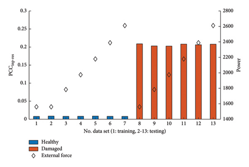
Figure 4 illustrates the results obtained when evaluating the resulting estimation errors, or more precisely the MAEs of the autoencoder for different magnitudes of excitation. With a similar excitation intensity, data set No. 2 has approximately the same reconstruction error as the learning file (data set No. 1), implying that the neural network is well trained.
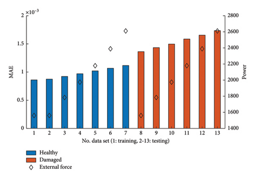
In principle, two findings can be derived from the results regarding the reconstruction errors of the model. Here, the anomaly score perfectly correlates with the average excitation intensity, making it unhelpful for anomaly detection. Secondly, the general differences between the damaged state and the healthy reference are also relatively small, making it difficult to discriminate health states. Impressive improvements in damage detection can be achieved when analyzing the input-residual correlations as shown in Figure 5. There is no dependence on the power of the excitation signals here. The reason is the amplitude-related normalization via the standard deviations, which was carried out by employing equation (7). Interestingly, the two damage indices (MAE and PCCinp−res) are evaluating the same autoencoders’ residuals and the results obtained differ significantly. These observations make the use of input-residual correlations a promising improvement for the application of autoencoders for damage detection.
3.3. Damage Localization
As mentioned earlier, the objectives of damage analysis in SHM are hierarchically structured, making higher levels more difficult to reach. Comparing measured signals for fluctuating excitation forces involves diverse excitation intensities. As presented, changes in amplitudes can lead to difficulties in detecting structural damage when evaluating the mean of the autoencoders’ errors. Therefore, similar excitation intensities must prevail for evaluation or the analysis must undergo some form of amplitude-related normalization. As described earlier, the normalization strategy is applied when evaluating the model’s residuals and dividing the input-residual correlations by their standard deviations. However, for damage localization, sensors are compared with each other to narrow down the damage position to adjacent sensors within a period, in which the system can be assumed to be stationary and time-invariant. Amplitude-related normalization is not mandatory here but the scaling of the absolute values can be applied to better illustrate the results, as carried out in this work.
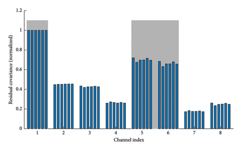
The six data sets classified as damaged are examined below for the associated damage positions. Changing excitation intensities are not affecting the outcome of the damage localization method as shown in Figure 6. When evaluating the residuals of the model using the residual covariances, the localization is not dependent on the power of the excitation. Although the absolute values of the residual covariance change, the relative correlations remain almost the same as shown in the figure. For better illustration, the values within a data set are normalized to 1. The results suggest that the model mainly learns the dynamic properties of the system and dependencies uncorrelated to the excitation force. As mentioned earlier, the underlying assumption is that the reconstructed signal of the sensor closest to damage differs most significantly from its actual measurements. In the given case, channel indices 1, 5, and 6 obtain the greatest values as they are closest to the two induced damages highlighted in gray.
Noteworthy, the method can be applied in a more complex failure mode such as two damage positions simultaneously. This is not a matter of course, as the changes in rigidity affect the entire system. Further damage positions are not included, as every possible damage position of the three-degree-of-freedom system for two different excitation positions has already been examined in [24].
4. Experimental Studies
Previously, the investigations focused on the proposed method for damage detection and localization using simulated data sets. While simulation studies and laboratory experiments provide valuable insights for method development, they do not fully capture the variability in real-world scenarios, such as nonlinearities, environmental factors, and measurement errors. The challenge lies in implementing this methodology in practical applications of SHM, where validation and insights into real-world feasibility are critical. By conducting this research in a realistic setting, the goal is to validate the proposed methodology and gain a quantified understanding of its potential in vibration-based SHM. To this end, the lattice tower equipped with a comprehensive monitoring system and subjected to varying environmental conditions [34] is described. The training of the autoencoder is depicted in the following. Over two weeks, structural changes were induced at three different locations to facilitate damage detection and localization. The results obtained are compared to different data-driven models and discussed for completing the validation studies.
4.1. Leibniz University Structure for Monitoring (LUMO)
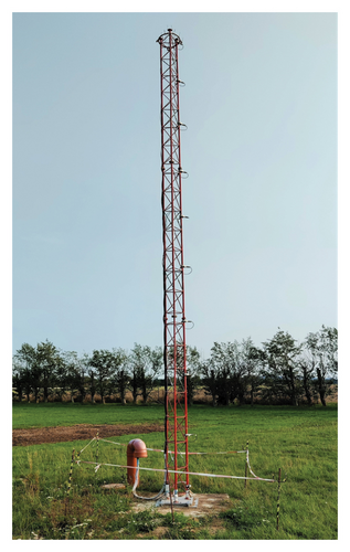
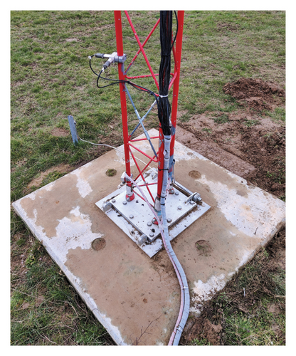
LUMO is situated in the state of Lower Saxony (Germany) near Hanover. The long-term monitoring-equipped lattice steel tower offers realistic environmental effects as it is located outdoors. Figure 7 illustrates an image of the experimental campaign, which comprises actively removing the lattice structure’s diagonal struts at several locations. Eighteen unidirectional accelerometers are strategically positioned across nine measurement levels (ML1–ML9) connected to a robust and protected acquisition system for response measurements. The damage positions (DAM1 through DAM6) are distributed over the tower’s height with the purpose of causing damage locally. Damage in the LUMO structure is induced by deliberately loosening M10 coupling nuts, causing targeted bracing elements to detach and thereby reducing overall stiffness. This setup allows for instant and repeatable removal of damage configuration when required. Figure 8 presents a detailed visualization of the damage mechanism associated with DAM6.

LUMO’s exposure to outdoor states contributes to its sensitivity to wind-induced aerodynamic forces. Thermal fluctuations, both diurnal and seasonal, significantly impact the structural characteristics of the dynamic system. For further interest, the reader is referred to the original publication in [34]. To provide a better understanding of the inspected damage patterns, Table 2 illustrates the identified natural frequencies utilizing the stochastic subspace identification initiated by Van Overschee and de Moor [35, 36]. The examined damages exhibit a significant reduction in stiffness, evident in the natural frequencies. As the height of the damage position increases, the change in natural frequencies generally decreases, as damage further down has a greater influence.
| Name | Noise level (SNR) (dB) | Pos. | B1-y (Hz) | B2-y (Hz) | B3-y (Hz) | B4-y (Hz) |
|---|---|---|---|---|---|---|
| Healthy | 20 to 60 | — | 2.77 | 15.98 | 40.89 | 69.21 |
| (a) | 20 to 60 | Level 6 | 2.75 | 14.30 | 33.90 | 61.16 |
| (b) | 20 to 60 | Level 4 | 2.76 | 15.90 | 37.49 | 64.95 |
| (c) | 20 to 60 | Level 3 | 2.76 | 16.07 | 36.72 | 65.63 |
- Note: Due to different excitation intensities, data sets have different noise levels. Within a data set, the noise levels also differ depending on the natural frequency under consideration, so that only a range is specified here.
4.2. Training of the Autoencoder
To effectively train an autoencoder for different temperature conditions, it is necessary to diversify the training data and use data sets that include input data corresponding to various temperature states. The neural network learns to encode the input data in a way that captures the underlying patterns or features associated with different temperature conditions. For every learning period, 20 × 10 min data sets were selected to map the structural temperature variations. For this purpose, the data sets were classified according to their mean temperature. Data sets were summarized at approximate intervals of 1.5°C (2.5, 4, 5.5, 7, …°C) so that the training data contain major parts of the temperature variations. Table 3 provides an overview of all data sets acquired from the structure and their corresponding temperature ranges. The three-stage damage analysis procedure is divided as follows: training and validation under healthy conditions, followed by testing under damaged conditions.
| Name | Training | Validation | Testing | No. of 10-min data sets |
|---|---|---|---|---|
| (a) | 7.1°C–27.4°C | 5.6°C–28.1°C | 2.2°C–26.4°C | 20/1201/1973 |
| (b) | −0.5°C–25°C | −0.5°C–25.1°C | −2.3°C–23.7°C | 20/1194/2133 |
| (c) | 7.1°C–27.4°C | −4.4°C–21°C | −3.1°C–22.4°C | 20/1199/1800 |
A longer sequence length is not advantageous in the numerical study due to the simulated permanent excitation by white noise with a constant power spectral density.
There is a fairly high linear dependency within the residual time series for a small number of principal components, as seen in Figure 9. As the number of principal components increases, the linear dependence between the residuals decreases and then increases again. For better differentiation, only eight of 18 sensors are visualized. The results imply that between 3500 and 4500, the errors consist mainly of highly uncorrelated noise components. Given these observations, the whiteness property is suitable for estimating the best number of principal components. It can be deduced that the test statistic of the common whiteness test increases more significantly with uniform excitation as seen in the simulation model. However, regarding real structures with variable environmental conditions, there is a larger range for optimal bottleneck dimensioning. The under- and overfitting due to the number of neurons in the smallest layer is particularly dominant for very large (1–50) or almost no data reduction (5300–5399).
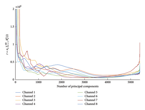
A meticulous approach is employed to determine the optimal bottleneck dimensions over three different periods used for training. In the scenario of damage case (a), analysis reveals a strikingly low correlation in estimation errors, particularly evident at 4055 neurons within the smallest layer, relative to an input size of 5400. Interestingly, beyond this threshold, the number of principal components—specifically, in channel 7—experiences a noteworthy surge (cf. Figure 9). Repeating the procedure for damage case (b), the neural network architecture search results in a bottleneck dimension estimated at 2631. Finally, for the third damage case, it is determined that the smallest layer of neurons for damage case (c) should comprise 2695 neurons, ensuring optimal performance and efficiency. Noteworthy, the identical trained model is utilized for both damage detection and localization purposes. Only the consideration of the residuals, by using two different input-residual correlations, changes depending on the level of SHM.
4.3. Damage Detection
Regarding the lowest level of SHM, the residuals of the trained autoencoder are analyzed and two damage indices are compared to validate the used methodology. Twenty data sets (200 min) are sufficient to train the model. Local stiffening due to the structure’s repair has been introducing unintentional irreversibilities so that the autoencoder’s training is repeated after each damage setup. Hence, the effort increases significantly because the learning process is the most time-consuming step of the calculation. Nevertheless, to mitigate redundancy, a more insightful validation of the vibration-based damage identification and localization under real-world conditions is executed. Each 10-min data set is evaluated using the autoencoders’ residuals by comparing their mean and the input-residual correlation quantified by a Pearson coefficient. In both cases, the evaluations result in a single value (or anomaly score) for every 10-min data set. The absolute value of each input-residual correlation (see equation (7)) is used to prevent negative and positive values from equalizing each other as described earlier. Thereby, the maximum value of the anomaly score does not exceed 1 and the lowest possible value is 0. The model’s evaluation period also presents the type I (false-positive) and type II (false-negative) error rates relevant for damage detection in SHM.
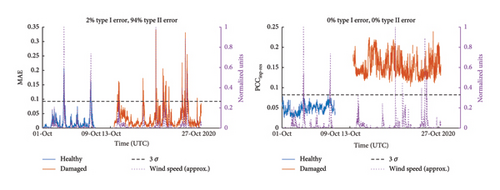
Figure 10 illustrates two damage indices—the reconstruction error of the autoencoder and the averaged input-residual Pearson correlation coefficients—when evaluating 10-min data sets of damage pattern (a). The damage-sensitive features reveal the changes related to the artificially introduced damage close to the platform. The figure consists of dots, each visualizing a different time step, which in the given case individually represents one 10-min data set. A dashed black line is added to highlight the three-sigma standard deviation of the healthy data. If the damage index exceeds this line, the corresponding 10-min data set is classified as damaged. In statistics, particularly in the context of a normal distribution, the mean (average) value plus or minus three standard deviations (3σ) encompasses approximately 99.7% of the data [6]. This range is used here to define normal variability and identify outliers. As the 3-sigma rule is straightforward to apply and easy to understand, it offers a comparison option between different models or damage indices. The horizontal axis represents the time in UTC, while the y-axis describes the damage indices. To identify the removal of all struts at damage level 6, the structural change can successfully be detected by comparing the linear correlations quantified by a Pearson coefficient PCCinp−res. Consistent with the simulation study, there is a clear improvement in contrast to the reconstruction error of the model. In the presence of changing environmental conditions, the variation in excitation in particular shows that an absolute value (MAE) is unsuitable for damage detection and that an amplitude-normalized damage indicator is necessary for compensation.
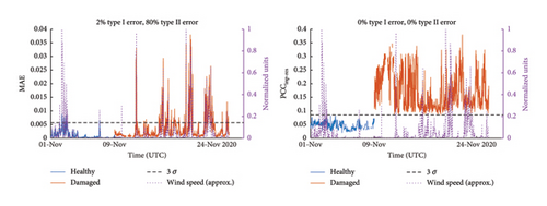
Damage pattern (b) involves the structural stiffness reduction in a higher position of the steel truss tower. The results obtained by computing both anomaly scores are visualized in Figure 11. Consistent with previous observations, the reconstruction error of the autoencoder evaluating raw time series is unsuitable for damage detection due to its dependencies on excitation intensities. In contrast, the structural change is detectable when considering the autoencoders’ inputs. It should be noted that the natural frequencies decrease less in the second than in the previous damage scenario (cf. Table 2) due to a higher positioning of the damage level. The overall stiffness of the system changes less than with damage pattern (a), but the local stiffness properties of the damage level, when removing all struts, are the same. The results thus imply that the autoencoder with input-residual considerations can reproduce this change correctly. The linear correlations quantified by Pearson coefficients have a mean value of 0.165, concurring with damage pattern (a), and an average value of 0.153 regarding all data sets from the damaged state. Notably, the variations of the PCCinp−res values obtained are quite strong and the quantification of damage needs to be investigated using varying severity at different damage levels.
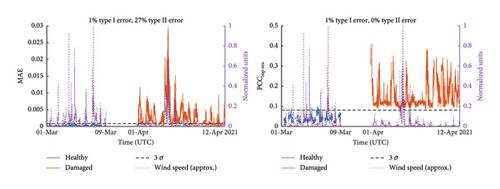
The findings pertaining to damage pattern (c) are depicted in Figure 12. The figure illustrates the damage-sensitive features for the damage-induced structural change between measurement levels 5 and 6. The reconstruction error of the autoencoder is unsuitable as a damage index, although the performance improves compared to the previous evaluations. Mainly due to the low wind speeds in March, the MAEs are generally quite small for the healthy state producing a smaller type I error rate. The separation of the two health conditions is again successful when looking at the PCCinp−res values. Despite the higher positioning of the damage level, the values quantified by a Pearson coefficient to detect the structural change have a mean of 0.15 and correspond to the previous damage patterns (0.165, 0.153). As mentioned before, these findings regarding the severity of the structural damage need further investigations, such as simulation studies and laboratory experiments, as EOC-dependent variance can be neglected here.
4.4. Damage Localization
The approach is based on the expectation that the sensors positioned nearest to the damage register the highest scores. With two acceleration sensors deployed at every measurement level, their residual covariances calculated as defined in equation (8) are averaged. Sensors farther from the damage position are expected to show no significant values. To consolidate the findings effectively, only the mean values of each measurement level are reported. If one measurement level has continuous highest values for each file, the residual covariance of the measurement level is 1 or 100%. Additionally, the frequency of maximal values for each measurement level is illustrated. A total of 1973 (a), 2133 (b), and 1906 (c) 10-min data sets are evaluated; accordingly, all available data sets in the induced structural change period—even those with very low wind speeds—are given to the autoencoder.
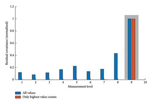
Figure 13 illustrates the autoencoder’s evaluation score (cf. equation (8)) when testing 10-min data sets of damage pattern (a), more precisely, the entire removal of damage mechanisms in the vicinity of the tower’s concrete foundation. The figure consists of bars each representing the values for a different measurement level. A gray box is manually embedded within the bar plot figure to explicitly highlight the position of the alteration. The horizontal axis represents the measurement levels (as defined in Figure 7), while the vertical axis represents the residual covariances. To identify the removal of all damage mechanisms at level 6, the residual covariances are normalized, so that the maximum absolute value is set to a value of 1 for each data set. The values are then averaged over the 10-min data records to assign one value to each measurement level; these values can have a maximum of 1 due to the previous normalization. The highest values are assigned to measurement level 9, closest to the location where the first damage occurred. Notably, without any exception, the value at measurement level 9 is highest for all 10-min data sets showcasing an excellent model’s performance. Measurement levels 2, 6, and 7 show exceptions to the decreasing pattern observed at increasing distances from the damage. However, these values obtained are comparatively small and are therefore not further to discuss.
As before, the dynamic response measurements change due to caused structural modifications. For damage pattern (b), the results of the time series-based model are visualized in Figure 14, in which the residual covariance serves as a damage position indicator by evaluating the autoencoder’s input-residual correlations. A steady increase in residual covariance emerges as the location becomes progressively closer to the damage site. This trend holds true, showcasing a gradual decline in values as one moves further away from the damaged area. Measurement level 6 appears to be much less dominant than level 7, which does not correspond to the damage mechanism being closer to measurement level 6. One possible explanation for this overemphasizing is LUMO’s constrained boundary condition below, which gives the dynamic system the opportunity for free vibrations at the top. This imbalance can introduce inconsistencies in the evaluation method, slightly overestimating higher measurement levels of tower structures.
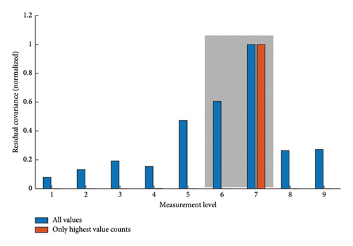
Figure 15 presents the results related to the third structural modification, located between ML5 and ML6, referred to as the study’s damage pattern (c). The damage position can be narrowed down to the adjacent sensors closest to the damage level 3, illustrating accurate localization results.
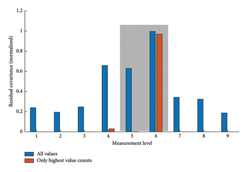
Consistent with earlier observations, the anomaly scores obtained are particularly high for signals acquired on levels that are near the removed struts. Interestingly, measurement level 6 dominates the evaluations conducted, although the damage is the second closest measurement level to damage level 3. As mentioned earlier, the boundary conditions of the structure seemingly influence the model’s output. Measurement level 4 rarely shows maximum values in the comparisons of residual covariance due to its close distance to damage level 3 (cf. Figure 7).
4.5. Comparison to Other Data-Driven Models on LUMO
Particularly appealing is the idea of comparing different data-driven models on identical measurement data to review the individual method’s performances. LUMO is well-suited for this task as it offers a free accessible benchmark. The monitoring structure was installed in mid-2020 for long-term data acquisition and has been continuously supplying data to the measuring system since then. The freely accessible data have been analyzed by various scientists, in particular, using data-driven models in vibration-based SHM. By mid-2021, three symmetrical and three asymmetrical damage scenarios had been investigated. Due to the low torsional stiffness of the structure, asymmetrical damage scenarios have played a subordinate role to date. Hence, the comparison with other data-driven methods focuses on symmetrical damage, the damage patterns (a) to (c) from this work, as described in Table 4. The table does not provide any information on the performance of the different data-driven methodologies in analyzing the damage patterns, only whether they were investigated. Regarding the table, this work can therefore best be compared to [11], as all damage scenarios for damage detection and localization were investigated.
| Author(s) | Damage patterns | Detection | Localization | Regression | Projection |
|---|---|---|---|---|---|
| Wernitz | (a)–(c) | ✓ | ✓ | (✓) | ✕ |
| Hofmeister | (a) | ✕ | ✓ | ✕ | ✕ |
| Römgens et al. | (a)–(c) | ✕ | ✓ | ✕ | ✕ |
| Kullaa et al. | (a) | ✓ | ✓ | ✕ | ✕ |
| This work | (a)–(c) | ✓ | ✓ | ✓ | ✓ |
- Note: The compensation of temperature effects is associated with a regression task; the amplitude-related normalization removes the influence of different excitation intensities by projection.
This study explores an innovative approach for damage localization within data-driven SHM, focusing on vibration-based techniques. By applying linear quadratic estimation theory, the authors present a method for identifying severe damage on LUMO. Only a third of the data was analyzed to shorten the long-term monitoring. Settings based on the frequencies and the Modal Assurance Criteria values were set, and a simple clustering algorithm for classification was applied. Precisely for damage pattern (a), the author used approx. 250 of 1973 data sets in the damaged state. A small number of incorrectly assigned data sets were found in both damage detection and localization. The method is especially valuable due to its physical derivation, but it needs improvements in the input-related normalization.
Hofmeister [37] investigated impulse response filters to identify the lowest induced structural change, namely, damage pattern (a) from this study, using the residual power as a damage-sensitive feature. The author aimed to extract more information from the measurement data by focusing on the performance of damage localization. The evaluation of the lattice tower included one 10-min data set for learning and one 10-min data set for testing the method during similar conditions, more precisely a temperature of 11°C and a wind speed of 5 m/s. The approach showed little robustness regarding damage localization, and it was advised to use a multi-stage scheme for practical monitoring applications.
By evaluating autoencoders with non-standardized time series data, Römgens et al. [24] were able to localize the damages for every damage pattern. The realization was successful for similar wind speeds and temperatures, showing that the method is in principle well suited. Small autoencoder structures were used, and the model was trained on one 10-min data set. Further, it was found that due to the low torsional stiffness, the torsional modes in particular react very sensitive to non-symmetrical damage. This disturbed the localization results, and there were large differences in the undamaged structure, particularly at the upper damage levels. Damage detection using the residuals of the autoencoder was not addressed in this study.
Autocovariance functions employed on different signals, as described in [38], exhibit spatiotemporal dependencies to detect abnormalities. Applying these functions for damage detection and localization on LUMO data is particularly challenging due to the closely spaced modes. It was concluded that increasing the number of sensors is advantageous. Of the six cases mentioned, the paper focused on the lowest induced symmetrical damage, damage pattern (a) from this work. The damage localization has been successful in most regarded cases.
The study examined an extended measurement campaign aimed at facilitating real-life validation of an autoencoder-based approach for damage identification in SHM. Notably, the autoencoder outperforms the existing approaches working on the LUMO data. The robustness of the proposed method has been ensured by analyzing the autoencoders’ input-residual correlations. To show the robustness of the damage position indicator, the localization has been conducted for all data sets. However, due to the dependence on excitation intensities, very low wind speeds have not been included in the damage detection procedure.
4.6. Discussion
This study aims to show the increased sensitivity and robustness of the autoencoder, evaluating a significantly higher number of data sets than the previously mentioned works. Excluding data sets based on arbitrary criteria may introduce limitations in the validation and calibration of the SHM system. It is essential to carefully consider the rationale for excluding specific data sets and ensure that it aligns with the overall objectives and requirements of the monitoring application. In our regard, very low wind speeds typically result in minimal structural response vibrations, and because the objective of the SHM system is to detect anomalies or changes in the structural behavior under dynamic loading conditions, data collected during these events may not provide enough useful information. Thus, very low wind speeds (< 0.5 m/s) were excluded in the evaluation of the damage detection, and, e.g., due to this criterion for the first induced damage, 193 of 3174 data sets were disregarded. Otherwise, no further adjustments have been made. For damage localization, sensors are cross-referenced to pinpoint the damage location by identifying deviations between sensor readings within a defined period. It can be assumed that during analysis, the structural system remains stationary and time-invariant; as such, all data sets are evaluated for the procedure.
By applying the methodology to a simulation study, it was shown that the MAEs of the autoencoder are sensitive to amplitude changes and accordingly also dependent on the excitation of the structure, which is varied by adjusting the power of the input signals (cf. Figure 4). Due to the additional consideration of the autoencoders’ inputs, as depicted in Figure 5, the robustness and sensitivity of the evaluation method increase significantly. It has been shown that the excitation intensity is compensated by the linear input-residual correlations, which are quantified by a Pearson coefficient. Interestingly, both damage detection features strongly differ although the model is not adapted and the same residual time series are analyzed. Consistent with these observations, it was possible to assign all 10-min data sets, using the input-residual correlations, to the correct health condition for real-life validation of the method, as illustrated in Figures 10, 11, and 12. Naturally, the changes within the state of the structure are mainly related to the modal parameters of the system. It is assumed that the smaller the changes in the natural frequencies and damping of the system, the smaller the fluctuations in the damage indices. The autoencoder may have difficulty capturing all the variations if the states being learned are complex or diverse. It has been observed that the lowest values for damage detection are exclusively attributable to low wind speeds; a specific connection to the identification of natural frequencies is assumed here.
Figures 13, 14, and 15 visualize the evaluations using the input-residual covariances to identify the corresponding damage positions. The results obtained indicate the practical use of the evaluating metric, allowing for consistent identification of the damage positions. Further, the autoencoder-based approach perfectly reproduces the expected decreasing tendency as the distance from the damage increases despite the challenging but realistic environmental conditions. The autoencoder’s benefit lies in its computational structure, which compresses the information within the latent representation and is equally distributed to the autoencoders’ outputs. As a result, the autoencoder exhibits an excellent baseline to localize minor defects.
In our opinion, three essential factors contribute to the successful and efficient realization of the method proposed. First, sequences of non-standardized time series are employed as input variables to achieve a high sensitivity toward structural changes. We consider input-related modifications as avoidable for the purposes of retaining spatiotemporal dependencies. Second, due to the complex nature of deep learning models, the information density can still be processed in such a way that features are automatically extracted. Moreover, as mentioned earlier, the autoencoder structure implies independence of the excitation position because information is compressed in the latent representation [24]. Third, the input-residual correlations improve the sensitivity and robustness of the method proposed. The anomaly detection using the reconstruction error would have resulted in a poorly performing model, although the same autoencoders’ residuals were analyzed as with the input-residual correlations. This improvement is particularly clear in the simulation model, as ambient conditions and measuring equipment do not play a role here.
5. Conclusion
This study explored the utilization of an autoencoder-based approach trained on sequences extracted from raw time series for damage analysis under changing environmental conditions in vibration-based SHM. The autoencoder was trained with learning files that mainly contained the temperature variances, as these are environmental factors that influence the response of the real-life structure. It has been shown that the autoencoder can process this information and create a complete separation between healthy and damaged data sets despite the fluctuating environmental conditions. For the damage detection purpose, it was devised to use the input-residual Pearson correlations, which showed significant advantages over the reconstruction error evaluating the same autoencoders’ residuals. The correlations were used to avoid any external adjustments to the model—such as input-related modifications—and can be interpreted as an amplitude-related normalization accounting for different excitation intensities. It has also been shown that input-residual correlations can be used consistently for identifying the damage position. Amplitude-related normalization is deemed unnecessary in using data-driven models for identifying the damage positions, as opposed to damage detection methodologies. One drawback of the method proposed is the non-physical interpretability of the model. Further, the training process requires a reasonable range of environmental conditions to capture the temperature-dependent structural responses. In summary, applying autoencoders with non-standardized time series data using input-residual correlations promises to be a strong tool for damage detection and localization in vibration-based SHM. The dependencies of the environmental conditions can be efficiently extracted using diverse data sets for the training process.
The input-residual correlations should be applied to different data-driven models to compare this to the commonly used error metric. The study’s results are interesting as the transfer from linear to nonlinear systems is easier to conduct as the neural network is already a nonlinear model. Accordingly, extending the framework to cover nonstationary and nonlinear systems represents a pivotal direction for future research. In population-based SHM, deep learning models show good transferability due to their capability of generalization and the potential of autoencoders with time series data should be investigated here.
Conflicts of Interest
The authors declare no conflicts of interest.
Funding
The authors greatly acknowledge the financial support provided by the Federal Ministry for Economic Affairs and Climate Action of the Federal Republic of Germany within the framework of the collaborative research project Grout-WATCH (FKZ 03SX505B) and SMARTower (FKZ 03EE2041C).
Open Research
Data Availability Statement
The data set is openly available under the Creative Commons Attribution 3.0 license and can be accessed through the LUIS data repository (https://data.uni-hannover.de/dataset/lumo).


