Prestressed bridges’ performance is strongly dependent on the health state of their prestressing cables, but unfortunately, these structural components are hidden and cannot be assessed through visual inspections. Moreover, conventional low-energy methods, like operational modal analysis, are inadequate due to their inability to detect the nonlinear effects of the prestressing force on the response under heavy travelling loads. In this paper, a methodology exploiting the Hilbert–Huang transform (HHT) is investigated in which the bridge’s nonlinear constitutive force–displacement relationship can be reconstructed by analysing the traffic-induced dynamic response, which has the features of a short-time nonstationary and potentially nonlinear signal. HHT, thanks to its adaptability to complex behaviours, is suitable for treating such type of signals and makes it possible to trace the response properties at each time instance, thus allowing to correlate instantaneous values of deformation with the simultaneous instantaneous (tangent) stiffness in a one-to-one relationship. Starting from a previous introductory study, and with the aim of making the proposed approach suitable for real structural health monitoring applications, a comprehensive investigation is performed considering a bridge with dynamical properties in the range of interest and realistic traffic scenarios adequately describing the time series of travelling loads and relevant internal actions. In particular, three main issues are considered: (i) development of a refined probabilistic response model (to be inferred from data collected under service loads) capable to overcome troubles induced by the nonhomogeneous distributions of data, generally consisting of frequent passages of light vehicles and rare passages of heavy vehicles; (ii) convergence analysis aimed at providing a relationship between the duration of the training period and the accuracy expected to infer the probabilistic model; and (iii) proposal and validation of a novel procedure to derive constitutive model of the bridge exploiting only deformation data recorded during vehicle passages and provide a tool for relating prestressing losses to variations in the dynamic response. The outcomes prove the potential of the proposed strategy paving the way for real-world experimental applications.

1. Introduction

This study focuses on the identification of the mechanical properties in post-tensioned reinforced concrete structures, with particular attention to bridges with decks composed of parallel beams connected by a reinforced concrete slab. These structures are prestressed using internal tendons encapsulated in protective sleeves, and later connected to the structure via grouting after the tendons are tensioned. The prestressing force significantly impacts the load capacity of post-tensioned reinforced concrete bridge decks, and its assessment is crucial because the degradation of these bridges [1–3], commonly built in the 1970–1980s, is often linked to the state of the precompression system.

While the prestressing force and cable path are designed to limit cracking under service conditions [4, 5], long-term effects like concrete creep, shrinkage, steel relaxation, and corrosion can reduce the prestressing force and introduce nonlinearity in the structure response under load.

The health state of the cables is difficult to be assessed through visual inspection alone [6–9], and moreover, monitoring the prestressing force is challenging, as conventional low-energy methods, like operational modal analysis [10], are insufficient due to their inability to detect the effects of the prestressing force on the system’s linear response. Indeed, as widely demonstrated in the past theoretical and experimental studies [11–16], the prestressing force does not affect the flexural stiffness in the linear response range, and a marginal influence can only be observed in more complex and higher (e.g., torsional) vibration modes.

The previous work carried out by the authors [17] established that the Hilbert–Huang transform (HHT) [18, 19] is potentially a powerful tool for the identification of the nonlinear behaviour of prestressed bridge from data obtained under service loads. The method does not simply detect deviations from a reference linear behaviour but makes it possible to recover the nonlinear relationship between deformation and internal actions, exploiting motion records only, without requiring information about the intensity of the travelling loads. It was observed that due to the local nature of the information provided by the Hilbert transform, with data showing significant irregularities in time, a statistical approach is needed for an unbiased interpretation of the results, and a generic approach was presented to define a probabilistic model from data.

However, although encouraging, these preliminary results called for a deeper investigation of the proposed method aimed at assessing its ability to identify the nonlinear response of prestressed bridges under more realistic traffic scenarios and to build up an effective monitoring system.

In this regard, the present paper pursues three main objectives: (i) the improvement of the accuracy and efficiency of the proposed probabilistic response model (to be inferred from data collected under service loads), taking into account the actual statistics of data coming from traffic and by overcoming troubles due to nonhomogeneous distribution of data, generally consisting of frequent passages of light vehicles and rare passages of heavy vehicles; (ii) the assessment of the convergence rate of the model parameters estimated from data series with different lengths in order to provide suggestions for the training period in realistic monitoring conditions; and (iii) the development and validation of a procedure to derive the nonlinear relationship between internal force and displacement of the structure exploiting only deformation data recorded during vehicle passages, with the final objective of providing a tool for relating cables’ prestress losses to changes in bridge’s dynamic response. The problem is approached by introducing a set of realistic traffic scenarios, where different vehicles typologies with diverse weights are considered, according to probabilistic models [20, 21].

A clustering method is proposed to recover homogeneous information at different amplitude of the dynamic response and balance the nonuniform distribution of the vehicle loads. Different parameters are considered for the clustering and relevant results are consequently compared.

Suggestions about the duration of the training period are also given by studying the convergence rate of the probabilistic model parameters under increasing numbers of vehicle passages, distributed according to their statistical models. Reported results concern the trend of the functions relating the instantaneous amplitude to the instantaneous circular frequency. The dispersion of estimated mean function and standard deviation function are reported and discussed, as well as the convergence rate of each model parameters.

Finally, the constitutive nonlinear behaviour of the system, describing the relationship between deformation amplitude and generalised internal action, is recovered from earlier analyses and the related results are discussed. Practical insights are also provided for a reliable usage of the proposed HHT-based monitoring approach, where typical drawbacks arising from the use of an empirical mode decomposition (EMD), such as the noise sensitivity and the so-called end-effects, are discussed and solutions tailored to the problem at hand are given.

The paper is structured as follows: Section 2 offers an overview on the existing literature concerning the structural health monitoring (SHM) of bridges and the typical time–frequency analysis techniques; the proposed novel methodology for the nonlinear response characterisation is recalled in Section 3; the considered benchmark case study is presented in Section 4 together with the traffic scenarios; the refined probabilistic model is presented in Section 5; results are presented and discussed in Section 6; practical recommendations to cope with typical drawbacks arising from the usage of the HHT-based monitoring approach are provided in Section 7; finally, the main conclusions are summarised in Section 8.

2. Overview on SHM and Time–Frequency Analysis Techniques

Bridges play a critical role within transportation and infrastructure networks. Their disruption can have significant socioeconomic consequences, and their failure can endanger people’s lives [22]. Maintenance thus plays a decisive role, and it is crucial to prevent bridges from developing damages or, at least, detect damages or anomalous behaviours at the early stages of their development. Traditional visual inspections are effective for spotting evident issues (shallow cracks, spalling, external corrosion), but they often fail to detect hidden or early-stage damage such as those interesting internal structural components (e.g., prestressing cables in bridges). To overcome these limitations, the field is shifting toward SHM, which leverages sensor technology and real-time data. With recent progress in sensing devices, data processing, and communication systems, SHM offers powerful tools for identifying damage, assessing structural conditions, and predicting future performance. This data-driven approach supports more informed decisions in areas like maintenance planning, structural design validation, and emergency response.

A thorough review of the most relevant and recent progresses in the field of damage identification methods for bridge structures within the last decade can be found in [23], where more than 200 articles are identified and discussed, the interested reader can refer to it for more details. Although the literature is rich of studies on SHM for bridges, studies focussing on the specific typology of prestressed concrete bridges are quite scarce, despite this represents a critical area of research, given the widespread use of these structures—prestressed concrete bridges constitute a significant portion of the existing infrastructure—and the potential for hidden damage, which can remain undetected until failure occurs. The most relevant studies on the topic are briefly recalled below. The main challenge when dealing with such type of bridges is the identification of prestressing losses, and various approaches have been developed to this aim (e.g., [24–29]) adopting methodologies which are based on the use of a wide variety of measures and each one of them is characterised by specific technical requirements that can hamper their use in real-world applications [30].

An efficient and noninvasive monitoring strategy able to provide information on the health state of prestressed bridges without recurring to specific instrumentations and without needing to close (even temporary) the bridge is to date not available, and this motivates the research presented within the current paper which exploits the ability of the HHT analysis to retrieve detailed information on the instantaneous variation of the system stiffness.

In order to clarify the reasons behind the choice of using HHT, a brief overview and comparison is provided upon the three main time–frequency analysis techniques commonly applied to SHM [31]. These are short-time Fourier transform (STFT) [32], wavelet transform (WT) [33], and HHT [19]. It is all about the capability of these tools to handle nonlinear and nonstationary signals. Starting from STFT, it tries to handle the nonstationarity by using a fixed window size, hence accepting a trade-off between time and frequency resolution (the larger the time window, the better the frequency resolution, the worse the time resolution). This means that STFT struggles to capture rapidly changing frequencies because it smears the frequency components over time.

Unlike the STFT, the WT uses variable-sized windows (multi-resolution analysis) and can better handle nonstationary signals, but it still assumes that within each window, the signal keeps some degree of stationarity (i.e., locally stationary) to accurately capture its frequency content.

As recalled in [34], also in the wavelet analysis, time and frequency resolution depends on the selected scale factor: small-scale factors (i.e., more compressed wavelets) are suitable for detecting rapidly changing details of the signal, while high-scale factors are able to identify the coarse features. Moreover, WT assumes predefined basis functions (wavelets) which may not perfectly match nonlinear real-world bridge vibrations.

On the other hand, HHT is fully adaptive, there is no assumption of stationarity and an adaptive decomposition—EMD—is used to extract oscillatory-like features (intrinsic mode functions [IMFs]) from the data, to which the Hilbert transform can be applied to estimate subtle changes in frequency (this is obtained via the first temporal derivative of the phase angle of each IMF). This means that, to perform the HHT analysis, no specific information about the signal of interest is required, contrary to STFT and WT approaches, which require a priori knowledge of the signal for tuning some specific parameters (as an example window width, mother wavelet, scale factor) to the desired application.

It is worth noting that, despite they are all widely used powerful tools, HHT (hence EMD), STFT and WT are not interchangeable. They are quite different from each other, and whether to use one or another depends completely on the question one is trying to answer: if an overview of the spectral changes in power over time are of interest, then WT (or STFT) may be recommended, because it is ideal for finding a nice balance between temporal and frequency precision. However, estimating instantaneous frequency from WT is suboptimal because of frequency smoothing, and because wavelet assumes frequency stationarity during the time span of the wavelet, so that the estimate of instantaneous frequency would suffer from the lack of resolution and would not be possible to fit the trajectory of its time evolution [34].

Specialising this discussion to the context of the study at hand, it should be noted that the present study does not simply aims at measuring frequency variations, but it aims at establishing a relationship between instantaneous frequency, related to tangent stiffness, and instantaneous vibration amplitude, in order to recover the system constitutive behaviour. For doing this, it is fundamental to know precisely how the instantaneous frequency varies by time; hence, a significant resolution both of time and frequency is required, and HHT reveals suitable for this purpose because it allows to evaluate the instantaneous amplitude and frequency of IMFs in each sampling instant, thus allowing to correlate instantaneous values of deformation with the simultaneous instantaneous stiffness (tangent stiffness) in one-to-one relationship. Once the tangent stiffness variation over time is available, the constitutive behaviour can be obtained by integration.

On the contrary, approaches based on STFT and WT would tend to average this information over few oscillations making it impossible to use them to recover a constitutive behaviour, intended as a relationship relating deformation to response.

Details about the proposed HHT-based analysis methodology are given in the next section.

3. Data Analysis Based on HHT

This paper exploits the methodology proposed by the authors in the previous work [17] that allows us to detect the nonlinear behaviour of the bridge under heavy traffic loads even if the travelling loads are unknown.

The approach exploits the capability of the HHT [35] in extracting the instantaneous frequencies (more precisely, the derivatives of the phase angles, which change over the travelling time due to the nonlinear behaviour) from the dynamic vibration mode characterising the bridge’s response. This local information is then correlated with the measured displacements, to recover information on the current nonlinear elastic response.

Finally, because the Hilbert transform provides quasi-local information, the output of the analysis (in the frequency–amplitude chart) usually shows irregularities in time and the nonlinear patterns may result difficult to be highlighted or recognised. Hence, to cope with this issue, the authors proposed to derive a probabilistic model from the data by inference procedures. A probabilistic model makes it possible to catch how the local frequency distribution changes at different displacement levels.

The methodology depicted above is thoroughly detailed in the paper [17]; however, for the sake of clarity, a short recall of the main stages of analysis is summarised through the following bullet points:

i.
EMD of the deformation history, required to adaptively decomposed into a number of IMFs the monitored nonlinear and nonstationary signal (i.e., the bridge deflection time history) and thus select the pseudomode of interest, i.e., the mode carrying information on the system dynamic properties;
ii.
Hilbert transform of the extracted dynamic component of the motion, required to enrich the signal with its imaginary part and compute the phase angle, whose time derivative provides the instantaneous angular frequency of the system;
iii.
Correlation between the instantaneous frequencies and the simultaneous response displacement within a chart providing information on the system response nonlinearity;
iv.
Construction of a probabilistic model inferred, via maximum likelihood estimation, from the data of step iii, useful to ease the results interpretation and the identification of nonlinear patterns of the response.

The main limits of the proposed HHT-based strategy are those intrinsic of EMD ([36]), i.e., the sensitivity to noise (responsible for mode mixing issues during EMD), the so-called end-effects, and the low computational efficiency. There are solutions to mitigate or eliminate the first two issues, and they will be discussed in the dedicated Section 7. Regarding the computational cost, this represents an aspect impacting the possibility of real-time monitoring with HHT, which is not however within the objectives of the work.

4. Case Study and Traffic Scenarios

4.1. Bridge Model

The selected case study is representative of real existing precast bridges: it has a span length L = 35.0 m and a deck (Figure 1(a)) 10.60 m wide composed of 4 parallel beams of 2.20 m height each, connected on the top through an R.C. slab 0.30 m thick. The bridge properties can be summarised as follows: elastic modulus E = 35·10⁶ kN/m², inner damping ratio ξ = 2%, inertial moment J = 3.11 m⁴, area A = 5.4 m², material density ρ = 2500 kg/m³ (mass per unit length m = 15, 500 kg/m). Overviews of bridge stocks and typology statistics can be found in [37, 38].

Details are in the caption following the image — **Figure 1 (a)**
Open in figure viewer PowerPoint

Case study: (a) bridge cross-section geometry; (b) nonlinear elastic force–displacement constitutive law.

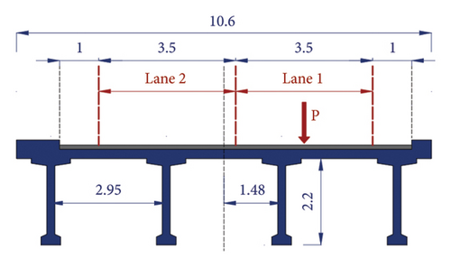
In this paper the response of the side beam on the right is analysed (Figure 1(a)), assuming a travelling loads sequence applied in the centre of the slow lane (Lane 1). Based on the deck geometry, and since transverse beams can be considered much stiffer than longitudinal beams, transverse load distribution can be studied through the classical Courbon–Engesser theory [39], according to which about 50% of the travelling load P is carried by the considered right-hand beam.

The dynamic problem governing the response of the beam under travelling loads is approached through the single degree of freedom formulation presented in [17], in which an approximate solution for the case of a system responding according to a nonlinear elastic constitutive law was derived. The solution is obtained under the assumption of a first mode-dominated response, which is generally acceptable when the midspan deflection is of interest, as in this case (in real applications, accurate measures of the bridge deflection could be achieved by remote monitoring via high-resolution cameras [40]). The fourth-order Runge–Kutta method [41] is used to provide a numerical solution of the problem. For further details on the formulation, the reader can refer to the work of [17].

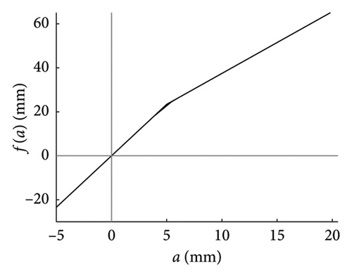
For what concerns the force–displacement law governing the beam response, the bilinear elastic one presented in Figure 1(b) is assumed in this study, as it can be seen as representative of a healthy prestressed beam under service loads close to the maximum considered design values.

The response amplitude is described by the midspan deflection a and the threshold governing the nonlinear transition is set equal to a^∗ = 5.0 mm The response is controlled by the stiffness ratio , with k₀ and k₁ identifying the first and second elastic stiffness, respectively. The sensitivity of the response with respect to the parameters a^∗ and k₁/k₀ has been discussed in [17].

As long as the system deflection maintains lower than a^∗, the first natural frequency of the bridge is ω₀ = 21.35 rad/s and the tangent stiffness is constant and proportional to ; the reduced natural frequency characterising the response in the second elastic branch is ω₁ = 16.54 rad/s.

4.2. Traffic Scenarios

Reliability and convergence rate of the model inferred by the maximum likelihood strongly depend on the statistical distribution of the available data. In order to discuss problems arising in a bridge monitoring and propose effective solutions, realistic traffic scenarios are considered.

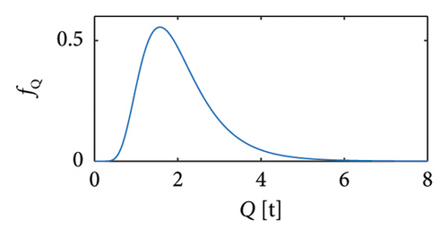
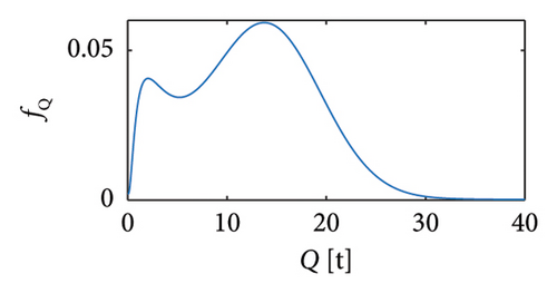
Sets of traffic scenarios are generated exploiting the mathematical distributions of random vehicle loads available in the literature (e.g., [20, 21]), i.e., stemming from the statistical processing of weight-in-motion (WIM) monitoring data relating to slow lanes of real highway infrastructures. In particular, the vehicle typologies listed in Table 1 are considered, each corresponding to a specific probability density function (PDF) (Figure 2) and characterising the whole traffic sequence proportionally to the values reported in column 2 of Table 1. To allow an explicit quantification of the minimum training period of a structural monitoring campaign, the inter-arrival times among vehicles are also modelled according to the Gamma distribution of Figure 3.

Table 1. Considered vehicle typologies and features.

Vehicle category	Vehicle typology	Proportions on the whole sequence	Relevant PDF (see correspondence in Figure 2)
Cat 1	2-axle car	0.5332	(a) Lognormal
Cat 2	2-axle bus	0.0642	(b) Lognormal + normal
Cat 3	2-axle truck	0.1597	(c) Lognormal + 2-peaks normal
Cat 4	3-axle truck	0.0958	(d) Lognormal + 2-peaks normal
Cat 5	4-axle truck	0.0833	(e) Lognormal + 2-peaks normal
Cat 6	5-axle truck	0.0738	(f) Lognormal + normal

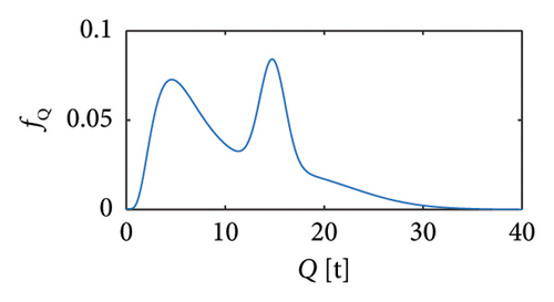
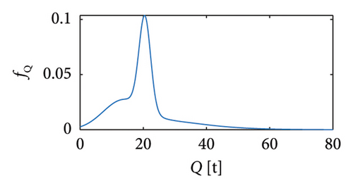
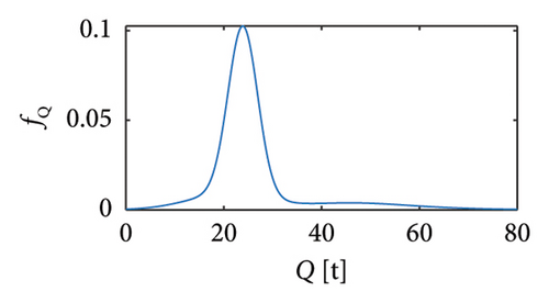
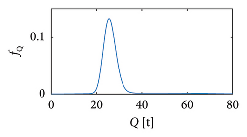
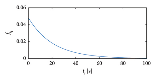
Regarding the velocities, they have been assumed as constant during the whole passage and according to the following assumptions: vehicles with gross weight Q < 3.5 t are considered travelling at the maximum velocity allowed by the National Highway Codes to date in force in Europe [9, 42], i.e., 130 km/h; vehicles with 3.5 t ≤ Q < 12 t travel at 90 km/h; the heaviest vehicles (Q ≥ 12 t) travel at 70 km/h.

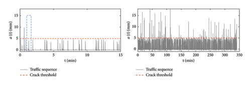
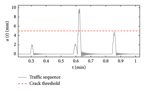
In Figure 4, two traffic scenarios are compared, one quite short consisting of 100 travelling vehicles (left charts) and a longer scenario consisting of 1000 passages. A detailed close-up of a typical response time history is shown in Figure 5.

5. Probabilistic Models (Improved) and Inference by Clusters

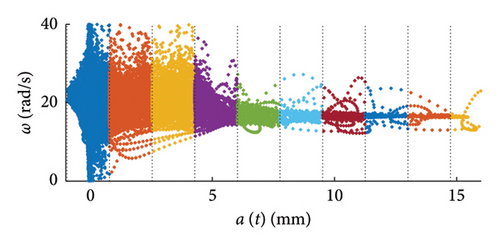
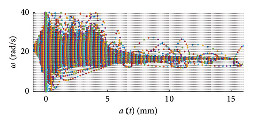
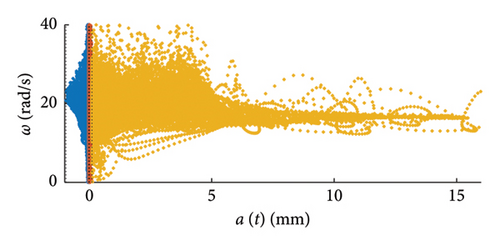
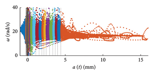
A frequency–amplitude correlation chart was proposed in [17] to highlight potential changes of the circular frequencies ω(a) with the amplitude a of the response, and in order to ease the reading of the plot (since Hilbert transform provides quasi-local information that may trace irregular paths), a probabilistic model was suggested. The model provides the PDF of the expected frequency conditional to amplitude a, and it can be inferred from the data to allow catching the changes of the frequency distributions with the displacement levels. This problem was solved in [17] exploiting a classic maximum likelihood optimisation, which revealed unsuitable in the current work because of the different structure of realistic traffic data, which consists of a majority of light vehicle passages producing low-amplitude responses which reflect in a unbalanced distribution of the dataset, showing a high density of points for low response amplitudes (left part of the chart) and a scarcity of data for high amplitudes (right part of the chart). This feature of the data can make the optimisation convergence harder and often biased results come out.

To cope with this issue a weighted maximum likelihood (WML) optimisation strategy is adopted, together with a clustering procedure of the data space. Furthermore, selected shape functions describing the variations of statistical parameters have been revised, according to outcomes from traffic data.

More in detail, defining the frequency and the response amplitude as random variables (RVs) (Ω, Y), their statistical features are described by the conditional PDF f_Ω|Y(ω|y; p), in which the pair (ω, y) represents the RV realisations while the vector p collects the characteristic parameters of the probabilistic model. Such model parameters can be inferred from the data by means of the maximum likelihood method, assuming the following, more expedient [43–45], log-likelihood objective functions L_ln(p):

()

where the pair (ω_m, y_m) denotes the m^th set of data observation from which the model provides the corresponding probability of occurrence.

The computation of the weights w_m to be applied to the objective functions of equation (1) is performed by dividing the dataset in a predefined number of clusters N_C (see Figures 6 and 7 for graphical examples), according to a predefined partitioning strategy [46], and by calculating the cluster weight w_Ci to be applied to all the pairs falling within the same cluster.

Two partitioning strategies have been proposed: (1) a uniform size partitioning approach and (2) and a uniform density partitioning approach (one could refer to this as quantile-based partitioning, being each cluster characterised by approximatively the same amount of data). Accordingly, the weights of equation (1) would assume the following expressions. For the uniform partition strategy:

()

where C_i represents the number of data points falling within the ith cluster.

For the quantile partition strategy:

()

where D_i represents the size of the ith equally dense cluster.

The weighted log-likelihood objective function defined in equation (1) can consequently be rewritten in its equivalent forms:

()

for the uniform partitioning approach, and

()

for the uniform density partitioning approach.

The two coefficients characterizing the PDF, i.e., the mean μ and the standard deviation σ of the distribution, are assumed to vary with the response amplitude according to properly selected shape functions, μ(y, p^μ) and σ(y, p^σ), being the model parameters collected in the vector p = [p^μ, p^σ].

The PDF of ω conditional to the amplitude y is assumed to be Gaussian, while the function adopted to describe the mean trend over the response amplitude y is a three-parameter Sigmoid function (equation (6)), which already revealed suitable in [17] to describe the particular nonlinear response of the system.

()

For what concerns the function describing the standard deviation, the linear relation (equation (7)) previously proposed in [17],

()

is now replaced with one of the following alternative nonlinear exponential relationships (denoted as Type 1 and Type 2, respectively):

()

which revealed both able (and equivalent) to follow the standard deviation changes, particularly in the transition interval between negative and positive displacements. Figure 8 offers a graphical comparison of the results provided by the three different standard deviation functions. Although the differences seem not significant, it shall be noted that the new proposed functions (equations (8) and (9)) allow to cope with the issue of negative standard deviations potentially induced by the use of the linear trend of equation (7), hence increasing the reliability of the probabilistic model.

6. Convergence Rate and Training Period

In this section, the convergence rate of the probabilistic model built via WML is assessed using a statistical approach.

For the purpose of these statistical assessments, a set of 100 independent simulations are performed for each case of analysis and the following metrics are introduced to assess the estimation error on the model parameters, specifically the mean (e_μ,i) and the standard deviation (e_σ,i) shape functions:

()

where μ_i(a) and σ_i(a) identify the mean and standard deviation functions for the ith case of analysis, while μ₀(a) and σ₀(a) denote the reference function for the mean and the standard deviation, respectively. These error measures are computed by numerical integration.

The results stemming from the probabilistic model can be used to reconstruct the nonlinear response of the bridge and provide insights into the prestress level of the beam. Indeed, the generalised internal force per unit mass of the system f(a)/m, corresponding (except for a scaling factor) to the term

in [17], can be found by integrating the ratio between the tangent stiffness k_t(a) = df(a)/dα and the unit mass m, which in turns coincides with the instantaneous angular frequency ω²(a), meant as the frequency of a small free vibration occurring in the neighbourhood of the deformation a. The integral can be expressed as follows:

()

This capability of the models will be assessed in the following and used as further metric to quantify the stability and convergence of the analysed scenarios.

The current section is organised as follows: in Section 6.1, a reference monitoring scenario is presented, made of an optimal choice in terms of time duration (number of passages over the bridge, N_V) and probabilistic model setting (i.e., number of clusters, N_C, for the likelihood function estimation); in Section 6.2, the influence of the partitioning strategy and related number of clusters, N_C, is assessed by keeping fixed all the other parameters at their reference conditions; in Section 6.3, the convergence rate of the probabilistic model under different traffic scenarios (in which the number of passages N_V is varied) is assessed; in Section 6.4, the capability of the model to reproduce the nonlinear relationship between internal forces and amplitudes is assessed; finally, in Section 6.5, insights for real monitoring applications are provided and the minimum training period for the model stabilisation is quantified.

6.1. Reference Optimal Solution

The reference scenario consists of a traffic sequence of N_V = 2000 vehicles. The number of clusters used in WMLE is set as N_C = 250, and a uniform partition strategy is used (despite identical results are obtained using a density-based partitioning approach with the same number of clusters).

The charts of Figure 9 show with thick red lines the average trends for the mean functions (a) and the standard deviation functions (b), while the related dispersions are identified through the grey dashed lines, representing the average ±one standard deviation. Moreover, two horizontal dashed lines are superimposed to the chart of Figure 9(b) to highlight the bounds of the expected variation interval of instantaneous frequencies ω.

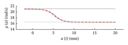
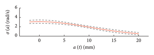
It can be observed how the dispersion of the mean functions is really low, while the fuse of the standard deviation functions is slightly wider.

Exploiting the probabilistic model, information about the changes of the instantaneous frequency can be inferred at any amplitude value of interest. For instance, using the average trends of the mean and standard deviation reported in the previous charts (Figure 9), the PDFs conditional to a set of increasing amplitude values can be estimated, as presented in Figure 10 (charts from a to f). From the inspections of these PDFs, the following points can be observed:

•
for low response amplitude values, the instantaneous frequency remains, on average, approximately constant and equal to the expected value ω₀ (i.e., the PDFs are centred on ω₀);
•
for rising displacements, the instantaneous natural frequency reduces below ω₀ and tends to stabilise on the value ω₁ for a > a^∗ = 5 mm;
•
the probabilistic model notably helps the graphical visualisation of such nonlinear pattern of the frequency–amplitude response;
•
the dispersion of the instantaneous frequencies decrease passing from small to high displacements.

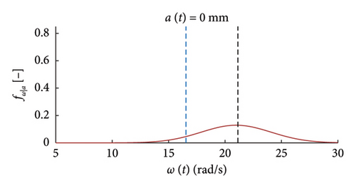
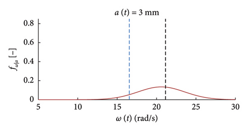
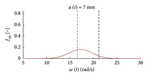
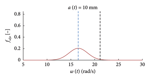
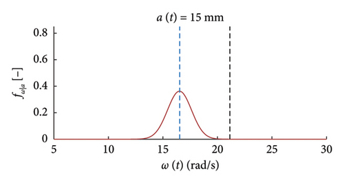
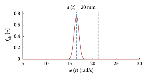
It can be seen how the probabilistic model provides a suitable tool for a clearer and faster extraction of information about the variations of the local dynamic properties with the response amplitude.

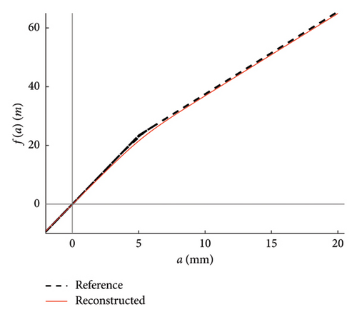
The advantage of the proposed tool is not limited to this, indeed the nonlinear constitutive law characterizing the system response can be retrieved by integrating the instantaneous frequencies (mean trend estimated through the probabilistic model) over the displacement amplitudes (according to equation (12)). For the case at hand, this result is shown in Figure 11 where the reconstructed response is compared to the expected reference law, testifying the goodness of the approach in terms of nonlinear response characterisation.

6.2. Influence of the Clustering Method on the Model Prediction

This section assesses the sensitivity of the probabilistic model to the clustering approach and, for the selected strategy, to the cluster size used to build the WML function. To this aim, the data generated from 100 simulations of traffic scenarios with N_V = 500 load passages is considered, while the number of clusters, N_C, is varied according to the following set of values: 10, 50, 100, 250, 500, 1000.

A box plot representation is proposed below to preliminary evaluate how the N_C values affect the results provided by the probabilistic models stemming from the 100 independent simulations, adopting a uniform clustering strategy or a density-based one. In particular, for what concerns the uniform clustering strategy, the statistics of the mean functions are presented in Figure 12, while those of the standard deviation functions are presented in Figure 13. For the alternative density-based partitioning method, results are shown in Figures 14 and 15.

Each chart shows, for different response amplitude levels (from −2 to 20 mm spaced 2 mm), a box plot representation of the interquartile range (IQR) (i.e., the distance between the third quartile and the first quartile), and a vertical black dashed line extending from the IQR indicating the range of frequency values exceeding the upper and lower quartiles; a red solid line shows the median trend, a red dashed line identifies the mean trend (these two curves are almost perfectly coincident in the majority of the cases).

In the charts of the mean functions only (i.e., Figures 12 and 14), two horizontal light grey dashed lines are added to highlight the bounds of the expected variation interval of instantaneous frequencies ω. This type of representation graphically aids to detect if the model provides biased results, indeed it is expected that, for low amplitudes, the frequencies are described by the upper dashed bound, while for high amplitudes, the frequencies should attain values equal to the lower dashed bound.

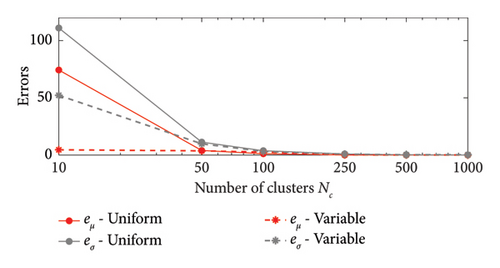
For a more quantitative assessment of the convergence rate, the error metrics defined by equations (10) and (11) are computed and reported in Figure 16 (red for the mean and blue for the standard deviation, solid lines for the uniform partitioning method, dashed line for the density-based one). Considering this and the previous charts, it can be observed that there are not macroscopic differences between the two partitioning approaches, and both are able to cope with the unbalanced distribution of data between low- and high-amplitude responses. More in detail, the density-based clustering shows a lower error rate associated to the estimation of the mean trend (good results can be obtained with less than 50 clusters), but the variance trends need at least 100 clusters to provide unbiased results; the uniform clustering approach has similar features, with a higher error rate for the mean trend estimation when less than 50 clusters are used. Overall, in order to produce stable results with both the uniform and density-based binning approaches, the use of N_C ≥ 100 clusters is recommended, with the optimal being N_C = 250.

Finally, the capability of the model to reproduce the internal force-amplitude constitutive law (equation (12)) using different clustering methods and cluster sizes is assessed. The results stemming from the use of a uniform size clustering approach with different N_C values are compared in Figure 17(a), where the reference theoretical solution is depicted in black dashed line. A similar comparison is made for the results stemming from the density-based clustering method in Figure 17(b).

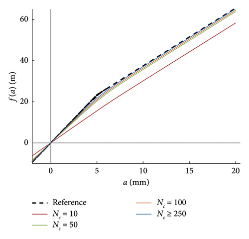
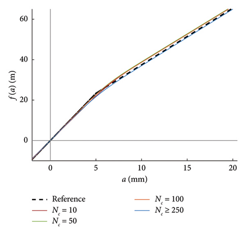
It is worth noting that, except for the case with 10 uniform clusters (Figure 17(a)), all the other cases provide reasonable approximations of the real nonlinear response, and particularly accurate is the outcome arising from cluster sizes equal to or higher than 250. N_C = 250 is thus assumed as best setting for the model within the following set of applications.

6.3. Convergence Rate of the Probabilistic Model

This section focuses on the assessment of convergence rate of the probabilistic model (estimated mean and variance functions) under different traffic scenarios, in order to quantify the model sensitivity to the duration of the traffic sequences and provide useful insights into its optimal training period (important for real monitoring applications). To this aim, different number N_V of vehicle passages are considered: 5, 20, 50, 100, 200, 500, 1000, 2000. The cluster size for the WML estimation is set equal to N_C = 250 according to the previous results, and again, in order to collect sufficient data for statistical analysis, 100 independent simulations are run for each selected traffic scenario.

The first assessment is performed mapping box plots at different response amplitude levels (from −2 to 20 mm spaced 2 mm), showing distribution/variability of mean (Figure 18) and standard deviation (Figure 19) functions estimates across 100 repeated simulations.

This plot summarises sample distributions providing, for each amplitude level, a box representation of the IQR (i.e., the distance between the 25th and 75th percentiles) and a vertical dashed line (whiskers) extending from the minimum to the maximum within that range (some whiskers are truncated by the upper and lower limits of the chart, to ease the reading of the plots). In these charts, the median and the average of the 100 estimated functions are reported using, respectively, red solid lines and red dashed lines. Moreover, to better check the stability of the solution, in the charts of the mean functions only (i.e., Figure 18), two horizontal light grey dashed lines are added to highlight the bounds of the expected variation interval of instantaneous frequencies.

Given that box plots do not provide confidence intervals (CIs) directly, a red shaded area is added to the charts to show the fuse within which the “true” result is expected to lie with 95% confidence, helping assess variability and stability of outcomes. Considered that a certain level of model instability arises when too short traffic sequences are adopted (N_V < 100 vehicles), and the outliers, even if a minority among the 100 simulations, notably affects the average trend (i.e., the mean of the simulations diverge pointing to systematic bias), the median of the estimated functions is used because of its higher robustness to extreme estimates and outlier runs, and for its capability to better reflect the central trend of the simulations. As a consequence, to reflect the uncertainty among the simulations, CIs are displayed around the median and are quantified using the order statistic method [47] (considered the nonparametric nature of the median) to ensure 95% confidence.

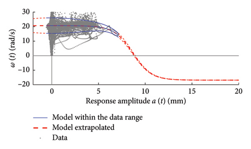
By analysing in detail the results of Figure 18, it can be observed how increasing the traffic size from N_V = 5 to N_V = 100 there is a visible improvement of the model predictions: the median trends tend to stabilise around the expected solution and the CI narrows considerably. Only for the shortest traffic scenario (N_V = 5), the pattern identified by the median is visibly incorrect, while for longer time series, it describes the correct patterns; on the contrary, as anticipated before and because of the nonnegligible sensitivity to outliers, the average trends reveal notably biased for traffic scenarios characterised by less than 100 passages, while they tend to stabilise on patterns very close to the median curves for longer traffic sequences (the two curves become identical for N_V ≥ 100). To understand the reasons of such an unstable trend of the average, an explicative case is presented in Figure 20, concerning a single specific simulation (an outlier among the 100 runs) from the traffic scenario with N_V = 50. From this figure, it appears clear that the estimated model (in blue solid lines) is well representative of the response within the interval of amplitudes of the raw data (grey circle markers), but it provides meaningless results (even negative frequencies) when extrapolated outside from this range (red dashed lines). The general conclusion stemming from this evidence is that too short traffic sequences, specifically traffic scenarios characterised by N_V < 100, are unlikely to contain vehicles sufficiently heavy to produce responses beyond the linear threshold, and as a consequence, the resulting model may be not robust enough to provide reliable estimation on a wide interval of amplitudes.

Considering this, and due to its higher stability, the median curves will be used in the following to assess the convergence rate of the models and capability to reconstruct the nonlinear constitutive laws of the system.

To recap, based on the information provided in Figure 18, N_V = 100 represents the minimum size of the traffic sequence size required to have sufficient stability of the model, with mean and median trends almost perfectly superimposed. However, traffic scenarios of at least N_V = 200 are needed in order to produce a significant reduction of the dispersion among repeated simulations. Higher traffic sequences (N_V ≥ 500) only produce beneficial reduction of the dispersion around the transition zone from the linear to the nonlinear branch of the curves (i.e., at amplitude levels around 5 mm).

Regarding the standard deviation functions (Figure 19), the dispersion regularly decreases as N_V increases and the trend of the median no longer changes (stabilises) from N_V = 100 onwards. The comments made above on median and average trends hold, and the N_V = 100 case represents the condition at which they start to be very close one each other.

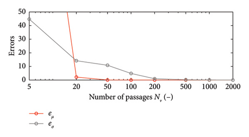
In order to quantify the convergence rate, the error metrics are computed according to equations (10) and (11) and reported in Figure 21 (red for the mean and blue for the standard deviation functions). Results confirm the conclusion that too short traffic sequences may affect the model stability, because the number of heavy vehicles collected within the data sample is not sufficient to catch the nonlinear response and the model built cannot be extrapolated outside the interval of calibration of the relevant parameters. Starting from 200 vehicles, the convergence rate is satisfactory (the errors are close to zero) for both the mean and the standard deviation functions.

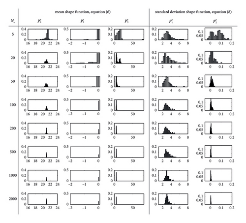
After having analysed in which way the traffic size affects the model global features (mean and standard deviation functions), the study is extended to explicitly assess the influence of N_V on the single model parameters. This is made in Figure 22 analysing how the model parameters distributions change varying the traffic size. In detail, the analysis is performed considering the three parameters (, , ) governing the (sigmoid) mean shape function (equation (6)) and the two parameters (, ) governing the standard deviation shape function (equation (8)). The outcomes of Figure 22 confirm the considerations made above according to which the real stabilisation of the model starts to become tangible for traffic sequences with N_V ≥ 100 vehicles, better if N_V ≥ 200. Moreover, it is worth noting that the dispersion of is generally larger than the dispersion of the other parameters, even if the dispersion regularly decreases by increasing the traffic size.

6.4. Constitutive Law Estimation

The capability of the models to reproduce the nonlinear relationship between internal forces and amplitudes is assessed exploiting the integration presented in equation (12).

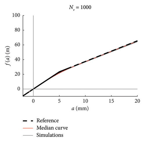
We can integrate the means of each of the 100 models, obtaining a bundle of curves, and discuss the median curve.

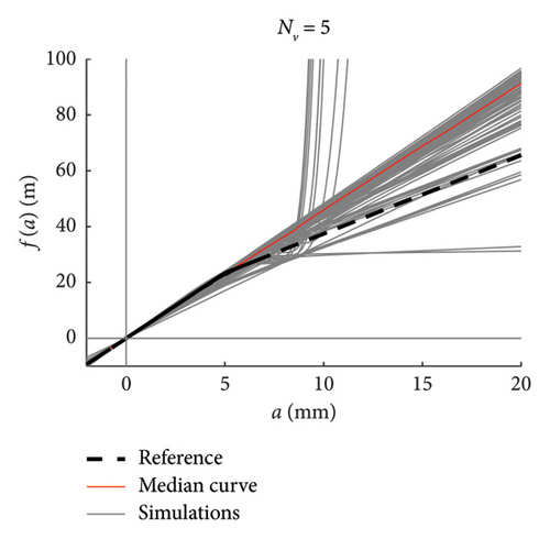
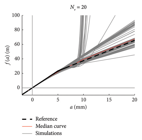
Recalling that there are 100 simulations performed for each traffic scenario (N_V), 100 constitutive laws are estimated by integrating the mean function of every model (100 models are available), hence a fuse of force–amplitude curves is made available for each case of analysis. These fuses are shown in Figure 23 using grey thin lines, and separated charts are presented for each case of analysis. The median curve is highlighted in red tick line and compared to the reference theoretical solution, depicted through a black dashed line. The following major comments arise from the observation of the figures. Traffic scenarios with 50 or less passages present curves with evident-biased trends, which are the direct consequence of the models’ weakness highlighted in the previous section and concerning the shortest traffic sequences. Despite this, the median curves are very close to the reference solution, with the only exception represented by the scenario with N_V = 5. From N_V = 100 on, the fuses are all regular and tend to tighten very quickly as N_V increases; indeed, from N_V = 500, all the fuses are hidden behind the median curve and their dispersion is almost null.

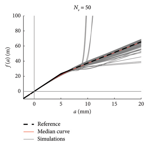
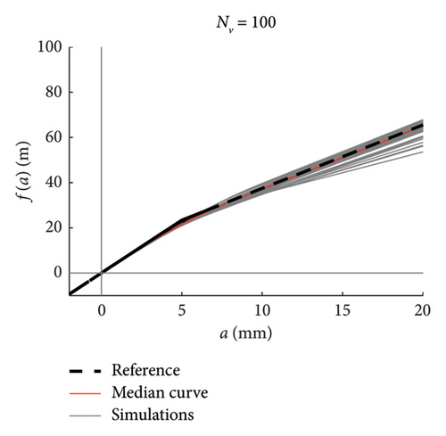
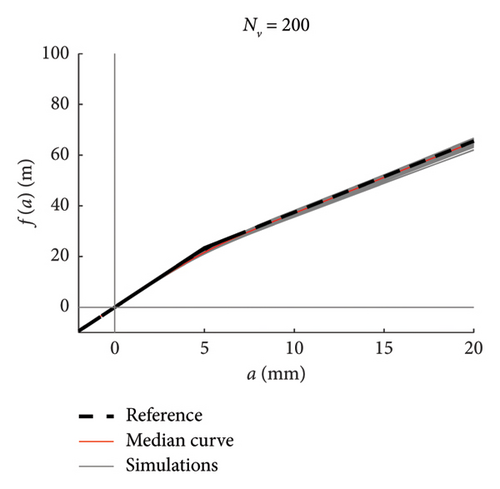
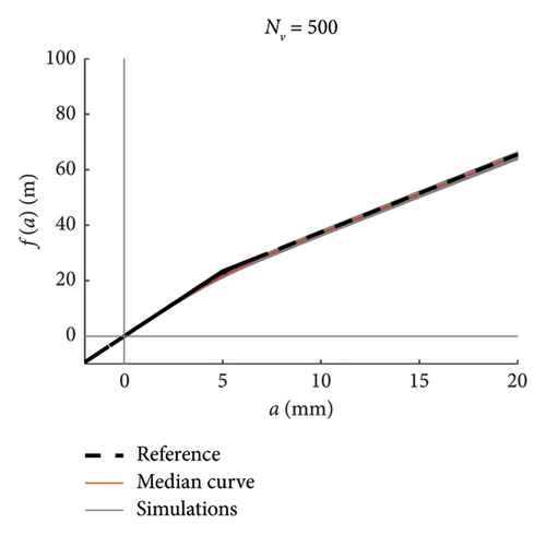
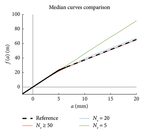
To ease the comparison between the median curves stemming from different traffic scenarios, these are superimposed in the chart of Figure 23(h).

It can be thus concluded that, in order to well reproduce the whole nonlinear behaviour in a stable and reliable manner, at least 100 vehicle passages are required, but N_V ≥ 200 is recommended to minimise the dispersion among repeated simulations (i.e., repeated measures in a real monitoring context).

As a final remark, it is worth noting that the internal force–amplitude relationships can be also derived from the integration of the raw data samples estimated from HHT, without passing through the probabilistic model. The outcome of a direct integration of the single simulated time histories is presented in Figure 24, where dedicated charts are provided for each considered traffic scenario.

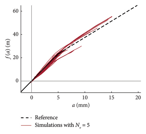
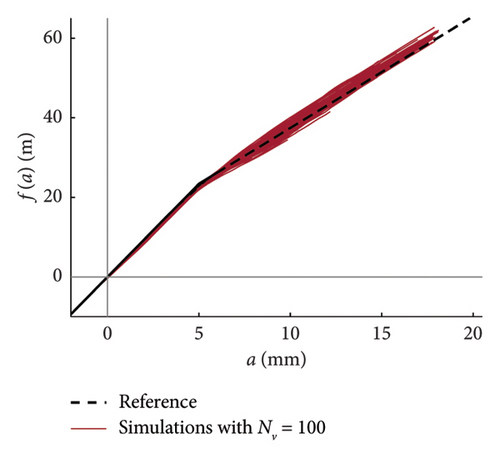
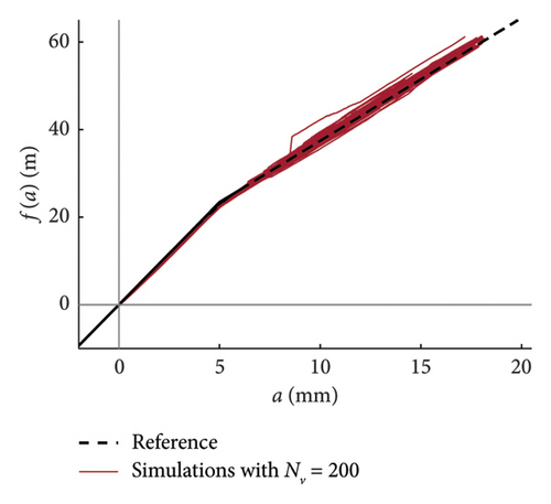
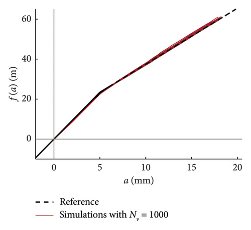
This strategy is particularly useful if the data sample is small (N_V ≤ 50), because it avoids biased estimation of the constitutive laws in those cases in which the observed responses are limited to the linear elastic range. On the other hand, passing through a robust probabilistic model would help avoid irregular trends and overcome the issue of having functions with different domains (the sample size changes at different amplitude levels). As said above for the curves derived from the model, N_V = 100 is the minimum traffic size required to adequately reproduce the system nonlinearity, with a quite regular fuse of curves and with a limited dispersion.

6.5. Training Period of the Model and Practical Recommendations

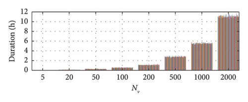
These results can be finally translated into recommendations about the minimum training period required to stabilise the model within a potential monitoring campaign of an existing bridge. To this aim, the correspondence between the temporal length and the number of vehicles characterizing each traffic sequence is provided in Figure 25. The recommended traffic size if N_V = 200, in order to produce stable and scarcely dispersed models, based on the outcomes extensively discussed before. Based on the durations reported in Figure 25 and in order to collect a sufficiently wide sample of response data from which extract a stable probabilistic model, the midspan deflection of the bridge should be measured for about 1 h, having care to choose the time window that presents the highest concentration of heavy traffic for the specific road section. It is worth noting that the value of observation time provided here is just an estimate based on the average traffic of a main road (i.e., approximately 200 vehicles/hour, for and average daily traffic of about 4000).

Although a single data recording, following the suggestion given above, can be sufficient to provide preliminary information on the system potential nonlinear response, it is advisable to repeat the measurements over a sufficiently long time frame in order to collect a set of independent measurements (let us say 100, to be consistent with the analysis setup proposed in this paper) on which calibrate a more robust probabilistic model (e.g., the median among the 100 responses could be used, as discussed above).

Based on these considerations and in order to set up a more robust monitoring campaign, the midspan deflection of the bridge could be measured for approximately 50 days by recording the data for about 2 h per day. A preliminary traffic analysis should be carried out to identify the daily hours with highest concentration of heavy traffic (this should be available if a WIM study has been performed on the road), otherwise, if a specific study is not available, the information may be derived from a direct observation (for a least one weak) of the daily traffic conditions. It is worth noting that the occurrence of anomalous traffic conditions might affect the convergence speed of the model, in particular the training time required to calibrate the model would slow down in case of very long light traffic periods. So, if particularly anomalous traffic periods are detected or expected (e.g., due to temporary bridge’s partial closures, road works, etc.), it might be better to temporarily interrupt the response recording waiting for a normal condition restoration.

To avoid collecting too long and heavy signals (the larger, the more computationally expensive to be processed, in particular via EMD procedure), the following recommendations could be followed: (i) the recorded time histories can be interrupted every hour, so that a pair of recorded signals would be made available every day; (ii) recordings can be limited to the working days only. Of course, there are other possible settings for the monitoring campaign which may differ from the one proposed above; in any case, the important aspect is that of ensuring a training period for the probabilistic model of about 100 h.

For what concerns the practical application of the suggested monitoring strategy, a cost-effective and noninvasive solution to perform the bridge deflections measurement, can be that exploiting high-resolution cameras whose accuracy proved to be competitive to that of classic transducers but with the advantage of eliminating any installation difficulty ([40, 48, 49]).

7. HHT-Based Analysis Challenges and Solutions

This section provides some practical insights for a reliable usage of the proposed HHT-based monitoring approach. In particular, the two main problems arising from the use of EMD are discussed in detail providing solutions and recommendations tailored to the problem at hand. The two issues regard the presence of noise in the recorded data (typical of real monitoring application) and the treatment of boundary effects during the empirical decomposition.

7.1. Handling Noisy Recordings

Noise can negatively affect the decomposition performed through EMD. Indeed, it is well known that mode-mixing problems (i.e., a single IMF consisting of signals of widely disparate scales or a signal of a similar scale living in different IMF components [50]) often occur when EMD is applied to nonstationary noise-containing signals, and this may negatively reflect on the subsequent Hilbert analysis.

Wu and Huang [51] proposed a noise-assisted data analysis method called ensemble empirical mode decomposition (EEMD), which suppresses the mode mixing problem of EMD by adding Gaussian white noise to the original data many times.

The capability of EEMD to deal with noisy signals has been evaluated extensively in the literature (e.g., [52]), and in this section, its suitability for the purposes of the current investigation is evaluated.

More specifically, two denoising techniques are tested in the following: a pre-processing approach via low-pass filter to denoise the signal before passing it through EMD, and the EEMD, which can be either applied to the filtered signal or to the original noisy one.

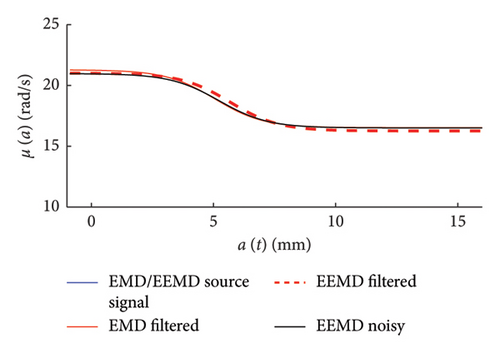
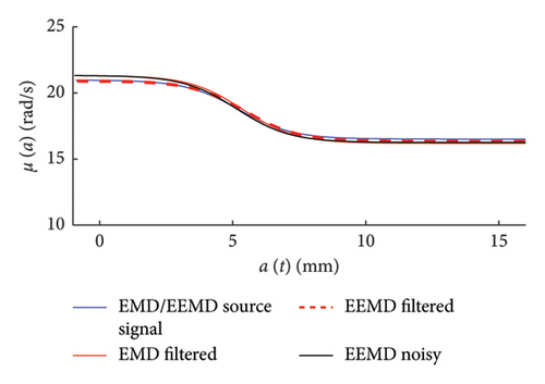
The low pass is built assuming a cut-off frequency of 10 Hz (62.83 rad/s) and a fourth-order filter. The EEMD is performed adopting a 10% noise level and a number of trials equal to 50, which provide a trade-off [53] between accuracy and computational time (the time required by EEMD-related algorithms increase when the number of trails is increased [54]).

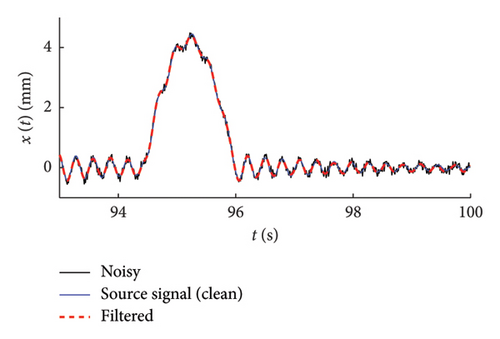
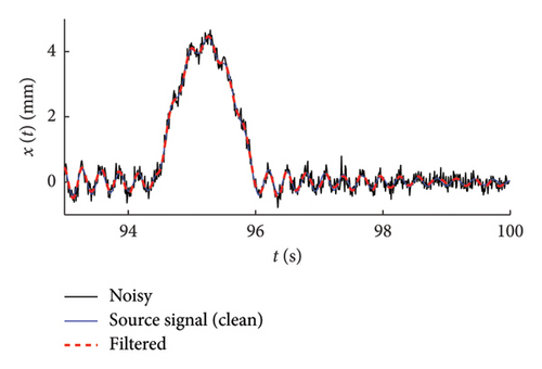
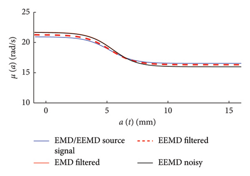
Three levels of noisy signals have been synthetically generated by adding a white-noise with different amplitude to an original source signal extracted from the traffic scenarios examined above (N_V 500 vehicles): low noise with a white-noise intensity equal to 0.1% of the maximum absolute response amplitude, medium noise (0.5%), high noise (1%). The set of noisy response time histories are shown in Figure 26 with specific close-up charts.

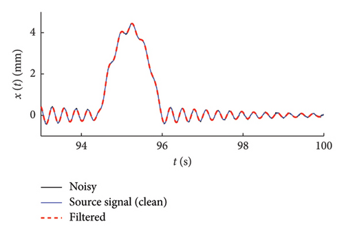
The effectiveness of the considered denoising strategies is assessed by comparing (Figure 27, right column charts) the mean functions of the frequency–amplitude probabilistic models built on the set of noisy signals. For the sake of completeness, in Figure 27 (left column charts), a close-up comparison is provided in the time domain between the noisy signal, the filtered one, and the original source signal (the one to which with noise has been added to produce the noisy time series).

Results can be summarised as follows:

•
Classic EMD procedure is not recommended for noisy signals due to the significant bias (mode mixing) occurring on the IMFs, even for very small level of noise (apparently negligible if observed in the time domain).
•
Traditional low-pass filtering approaches are able to solve this issue, so that the denoised signal can be safely processed through EMD or EEMD to obtain reliable results.
•
The EEMD procedure is an effective denoising alternative.

Other strategies could be considered to cope with noise in real bridge vibration problems, such as the combined usage of WT analysis as preliminary denoising means and HHT as core tool for the nonlinear response estimation of the system. However, this is out of the scope of the present work and will be investigated in future real-world applications.

7.2. Endpoint Problem Mitigation Strategies in EMD

One of the most significant challenges with the EMD approach is the treatment of end-effects. It is indeed recalled that, in EMD, IMFs are extracted by: (1) finding local maxima and minima of a signal; (2) interpolating the maxima to form an upper envelope, and minima to form a lower envelope, usually using cubic spline interpolation; (3) taking the mean of these envelopes to obtain a “trend”, which is subtracted to extract an IMF. But at the ends of the signal, there are no supporting points beyond the edges to properly anchor the spline. At the ends, indeed, one may only have a single local max or min, or no data exists beyond the boundaries to guide the spline shape, or also the spline may “swing” wildly to fit end points. In other terms, the existence of a signal at the application frontier of EMD has the potential to deviate the end-effects which may lead to a series of issues such as changing shapes of main envelopes, wrong and extra IMF, mode mixing, signal energy shifted toward the edges, and computational instabilities at the signal borders.

Among the existing strategies (e.g., see [55]), expanding the signal data is still the best basic approach for reducing end-effects. This expansion can be seen as a pre-processing of the signal according to one of the following strategies:

1.
Mirroring or symmetric extension, which consist of extending the signal by reflecting a few samples at each end, thus helping the spline interpolation by providing more data.
2.
Extrapolation, i.e., predicting values beyond the ends using local trends (e.g., polynomial or linear extrapolation).

An alternative way could be that using more stable interpolation techniques, e.g., switching from cubic spline to linear or monotonic piecewise cubic interpolation or others. Due to the relevance of the matter, the main methodologies to minimise distortions induced by boundary effects are discussed and compared with application within the context of the study at hand. The following strategies are considered: mirror padding (reflect start and end portions to extend boundaries), symmetric extension (reflect without inversion, smoother in some cases), linear extrapolation (add straight-line continuation at both ends). These three methods are also compared to the classic EMD procedure with no pre-processing of the signal.

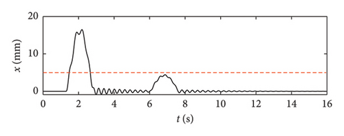
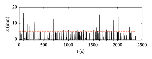
First, a very short-time nonlinear nonstationary signal is analysed, obtained by windowing a 16-s-long response time series from the database of bridge deflection responses analysed in this study. The signal is shown in Figure 28, and it is characterised by the exceedance of the crack threshold (shown by the red dashed line) for a limited interval of time (about 1 s).

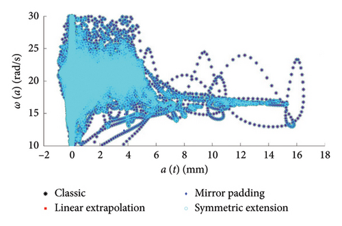
In Figure 29, the IMFs extracted adopting the classic EMD and the three alternative pre-processing strategies are presented, from which one can see how the boundary effects have a negligible influence on the first IMF, the only one of interest in this study. To further support this point, in Figure 30, the results obtained from the Hilbert processing of the IMF1, in terms of frequency–amplitude responses, are compared, and the differences among the datasets obtained using different pre-processing approaches are notably low.

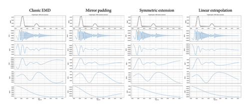
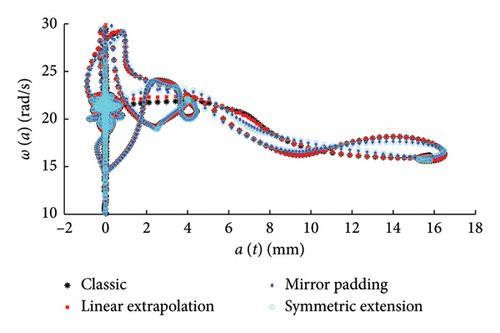
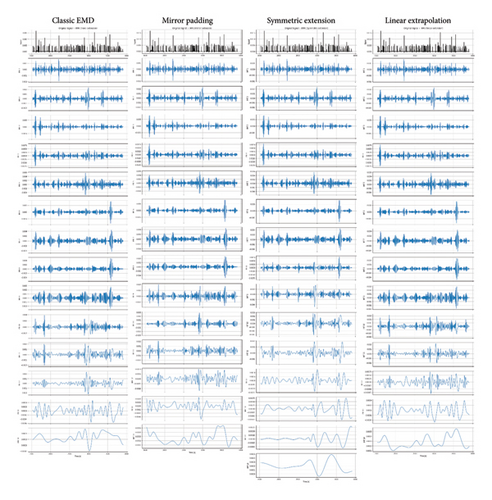
If rather than analysing small temporal windows, we do process the entire time series obtained from the traffic simulation with 500 vehicles (see Figure 31), we would further reduce the end-point effects: from Figure 32, it can be seen that only higher IMFs (from IMF 8 on) are affected by the adopted mitigation strategies, while the first 7 IMFs (and in particular the IMF1 of interest) are basically the same from all the compared strategies; this also reflects on the frequency–amplitude charts (Figure 33) where no differences can be appreciated among the four cloud of data estimated using different pre-processing approaches.

In conclusion, for the problem at hand in which only the first IMF is needed and by analysing long time series characterised by many vehicle passages, end-point effects induced by EMD are negligible. Moreover, approaching the problem through a statistical method (repeated measures and median extraction) might further reduce potential undesired distortion introduced by the EMD procedure. It has an outstanding performance in the processing of long nonlinear and nonstationary signals [6–8]. EEMD improves EMD by adding white Gaussian noise to the signal to eliminate mode aliasing because it could provide a relatively consistent distribution of referring size. After being averaged several times, the added noise will be offset, and the consistent scale component will be obtained. Wang et al. [56] had a detailed comparison between EMD and EEMD.

8. Conclusions

In this study, a methodology for the characterisation of the nonlinear behaviour of post-tensioned r.c. bridges is investigated. The approach exploits the abilities of the HHT in extracting the instantaneous properties of the dynamic response recorded on the bridge under service loads. With the aim of making the proposed tool available for real monitoring of existing bridges, this study performed some theoretical investigations where an analytical model of a bridge representative of the typology at hand is used and traffic scenarios are simulated according to statistical features derived from weight-in-motion records. The midspan deflection time histories are derived by numerically integrating the dynamic equations governing the problem of a nonlinear elastic beam under travelling loads. Considering that data collected through HHT-based approach typically present irregularities in time (because of the local nature of the information provided by the Hilbert transform), a refined probabilistic model is used to ease the results interpretation, whose parameters can be estimated via maximum likelihood estimation.

The main result of the present work is that the proposed approach can be effectively used to estimate the constitutive force–displacement relationship of the bridge by analysing the traffic-induced dynamic response. This reveals important for SHM of prestressed bridges because it allows retrieving information on the health state of their prestressing cables, which being hidden components cannot be assessed through visual inspections. Moreover, the proposed methodology overcomes the limits of conventional low-energy excitation methods, like operational modal analysis under environmental noise, which cannot be used for this purpose due to their inability to detect the effects of the prestressing force on the system’s linear response.

Based on the specific outcomes of the study, the following main general conclusions can be drawn:

•
The strategy proposed to identify a probabilistic model from real data coming from traffic scenarios is based on a clustering of collected measures which can be safely performed either through a uniform or density-based criteria (both the approaches are able to cope with the unbalanced distribution of data between low- and high-amplitude responses).
•
Parametric analyses show that at least 100 clusters are necessary to obtain satisfactory results, and further slight improvements can be obtained using an increasing number of clusters up to 250.
•
The shape functions selected for the probabilistic model are adequate and the model regularly converges increasing the data used for the inference problem or, more practically, increasing the time used for the training period.
•
Suggestions about the relationship between the duration of the training period and the accuracy expected for inferred probabilistic models are presented, and satisfactory results can be obtained with a number of vehicle passages larger than 100, while the model variability is negligible for larger number of passages.
•
A procedure to derive the nonlinear constitutive law between internal actions and bridge deformation is presented, and the result’s accuracy is discussed in a parametric analysis from which it is confirmed that with a number of vehicle passages larger than 100, the reconstructed response is very close to the expected reference one.
•
In order to implement the proposed procedures within a robust monitoring strategy of real bridges, a training period of about 100 hours is recommended to properly calibrate the probabilistic model parameters and have accurate predictions of the bridge’s nonlinear response.
•
A possible practical implementation could be that of recording the midspan deflection of the bridge 2 h per day (choosing the time window that presents the highest concentration of heavy traffic) for about 50 days.
•
To avoid collecting too long and heavy signals, the recorded time histories can be interrupted every hour and recordings can be limited to the working days only.
•
In the presence of noise, classic pre-treatment with low-pass filter or the use of a more efficient EEMD reveal both suitable strategies.
•
The proposed HHT-based methodology proved to have scarce sensitivity to the end-points effects potentially induced by the EMD; however, classic mitigation strategies can be used for preventive purposes.

Future works will be aimed at testing the proposed methodology in real-world experimental applications.

Conflicts of Interest

The authors declare no conflicts of interest.

Funding

The authors gratefully acknowledge funding from the Italian Ministry of University and Research through the PRIN Project “TIMING—Time evolution laws for IMproving the structural reliability evaluation of existing post-tensioned concrete deck bridges” (protocol no. P20223Y947), Prin PNRR, 2023-2026.

The work was also supported by “FABRE Research Consortium for the Evaluation and Monitoring of Bridges, Viaducts and Other Structures” through the project titled “SAFOTEB—a reviewed safety format for structural reliability assessment of post-tensioned concrete bridges”.

Open Research

Data Availability Statement

The data that support the findings of this study are available upon request from the corresponding author. The data are not publicly available due to privacy.

References

1 Wang L., Li T., Dai L., Chen W., and Huang K., Corrosion Morphology and Mechanical Behavior of Corroded Prestressing Strands, Journal of Advanced Concrete Technology. (2020) 18, no. 10, 545–557, https://doi.org/10.3151/jact.18.545.
10.3151/jact.18.545
CAS Web of Science® Google Scholar
2 Wang L., Strand Corrosion in Prestressed Concrete Structures, 2023, Springer Nature Singapore Pte Ltd.
10.1007/978-981-99-2054-9
Google Scholar
3 Podolny W., Corrosion of Prestressing Steels and Its Mitigation, PCI Journal. (1992) 37, no. 5, 34–55, https://doi.org/10.15554/pcij.09011992.34.55.
10.15554/pcij.09011992.34.55
Google Scholar
4 Hewson N. R., Prestressed Concrete Bridges: Design and Construction, 2003, T Telford.
10.1680/pcbdac.32231
Google Scholar
5 García-Segura T., Yepes V., and Frangopol D. M., Multi-Objective Design of Post-Tensioned Concrete Road Bridges Using Artificial Neural Networks, Structural and Multidisciplinary Optimization. (2017) 56, no. 1, 139–150, https://doi.org/10.1007/s00158-017-1653-0, 2-s2.0-85011880110.
10.1007/s00158-017-1653-0
Web of Science® Google Scholar
6 Federal Highway Administration-HRT-13-028: Guidelines for Sampling, Assessing, and Restoring Defective Grout in Prestressed Concrete Bridge Post-Tensioning Duts, 2013.
Google Scholar
7 Highways England, CS 465-Management of Post-Tensioned Concrete Bridges, 2020.
Google Scholar
8 Highways England, CS 464-Non-Destructive Testing on Highways Structures, 2020.
Google Scholar
9 Ministero Delle Infrastrutture e Della Mobilità Sostenibili, Linee Guida per la Classificazione e Gestione Del Rischio, La Valutazione Della Sicurezza Ed il Monitoraggio Dei Ponti Esistenti. (22A04700).
Google Scholar
10 Brincker R. and Ventura C., Introduction to Operational Modal Analysis, 2015, John Wiley & Sons.
10.1002/9781118535141
Google Scholar
11 Saiidi M., Douglas B., and Feng S., Prestress Force Effect on Vibration Frequency of Concrete Bridges, Journal of Structural Engineering. (1994) 120, no. 7, 2233–2241, https://doi.org/10.1061/(asce)0733-9445(1994)120:7(2233), 2-s2.0-0028467061.
10.1061/(ASCE)0733-9445(1994)120:7(2233)
Web of Science® Google Scholar
12 Dall’Asta A. and Dezi L., Discussion of “Prestress Force Effect on Vibration Frequency of Concrete Bridges” by M. Saiidi, B. douglas, and S. feng, Journal of Structural Engineering. (1996) 122, no. 4, https://doi.org/10.1061/(asce)0733-9445(1996)122:4(458).
10.1061/(asce)0733-9445(1996)122:4(458)
Google Scholar
13 Dall’Asta A. and Leoni G., Vibrations of Beams Prestressed by Internal Frictionless Cables, Journal of Sound and Vibration. (1999) 222, no. 1, 1–18, https://doi.org/10.1006/jsvi.1998.2066, 2-s2.0-0042706817.
10.1006/jsvi.1998.2066
Web of Science® Google Scholar
14 Dall’Asta A., Dynamics of Elastic Bodies Prestressed by Internal Slipping Cables, International Journal of Solids and Structures. (2000) 37, no. 25, 3421–3438, https://doi.org/10.1016/S0020-7683(99)00032-3, 2-s2.0-0033882457.
10.1016/S0020-7683(99)00032-3
Web of Science® Google Scholar
15 Noble D., Nogal M., O’Connor A., and Pakrashi V., The Effect of Prestress Force Magnitude and Eccentricity on the Natural Bending Frequencies of Uncracked Prestressed Concrete Beams, Journal of Sound and Vibration. (2016) 365, 22–44, https://doi.org/10.1016/j.jsv.2015.11.047, 2-s2.0-84955202461.
10.1016/j.jsv.2015.11.047
Web of Science® Google Scholar
16 Hamed E. and Frostig Y., Natural Frequencies of Bonded and Unbonded Prestressed Beams-Prestress Force Effects, Journal of Sound and Vibration. (2006) 295, no. 1-2, 28–39, https://doi.org/10.1016/j.jsv.2005.11.032, 2-s2.0-33646770340.
10.1016/j.jsv.2005.11.032
Web of Science® Google Scholar
17 Scozzese F. and Dall’Asta A., Nonlinear Response Characterization of Post-Tensioned RC Bridges Through Hilbert–Huang Transform Analysis, Structural Control and Health Monitoring. (2024) 2024, no. 1, https://doi.org/10.1155/2024/5960162.
10.1155/2024/5960162
Web of Science® Google Scholar
18 Huang N. E., Hilbert-Huang Transform and Its Applications, World Scientific. (2014) 16.
Google Scholar
19 Chen B., Zhao S. L., and Li P. Y., Application of Hilbert-Huang Transform in Structural Health Monitoring: A State-of-the-Art Review, Mathematical Problems in Engineering. (2014) 2014, no. 1, 1–22, https://doi.org/10.1155/2014/317954, 2-s2.0-84903584964.
10.1155/2014/317954
Web of Science® Google Scholar
20 Yang X.-Y., Gong J.-X., Wang Y.-H., Xu B.-H., and Zhu J.-C., Probability Model and Reliability Analysis of Cable Stress for Cable-Stayed Bridge, The Baltic Journal of Road and Bridge Engineering. (2017) 12, no. 4, 248–257, https://doi.org/10.3846/bjrbe.2017.31, 2-s2.0-85049742308.
10.3846/bjrbe.2017.31
Web of Science® Google Scholar
21 Lu N., Liu J., Wang H., Yuan H., and Luo Y., Stochastic Propagation of Fatigue Cracks in Welded Joints of Steel Bridge Decks Under Simulated Traffic Loading, Sensors. (2023) 23, no. 11, https://doi.org/10.3390/s23115067.
10.3390/s23115067
Web of Science® Google Scholar
22 G. Deodatis, B. R. Ellingwood, and D. M. Frangopol, Safety, Reliability, Risk and Life-Cycle Performance of Structures and Infrastructures, 2014, CRC Press, Boca Raton, FL, https://doi.org/10.1201/b16387.
10.1201/b16387
Google Scholar
23 An Y., Chatzi E., Sim S. H., Laflamme S., Blachowski B., and Ou J., Recent Progress and Future Trends on Damage Identification Methods for Bridge Structures, Structural Control and Health Monitoring. (2019) 26, no. 10, https://doi.org/10.1002/stc.2416, 2-s2.0-85069679288.
10.1002/stc.2416
PubMed Web of Science® Google Scholar
24 Hu W.-H., Tang D.-H., Teng J., Said S., and Rohrmann R. G., Structural Health Monitoring of a Prestressed Concrete Bridge Based on Statistical Pattern Recognition of Continuous Dynamic Measurements over 14 Years, Sensors. (2018) 18, no. 12, https://doi.org/10.3390/s18124117, 2-s2.0-85057150122.
10.3390/s18124117
Web of Science® Google Scholar
25 Sakiyama F. I., Veríssimo G. S., Lehmann F., and Garrecht H., Quantifying the Extent of Local Damage of a 60-Year-Old Prestressed Concrete Bridge: A Hybrid SHM Approach, Structural Health Monitoring. (2023) 22, no. 1, 496–517, https://doi.org/10.1177/14759217221079295.
10.1177/14759217221079295
Web of Science® Google Scholar
26 Abdel-Jaber H. and Glisic B., Monitoring of Prestressing Forces in Prestressed Concrete Structures—An Overview, Structural Control and Health Monitoring. (2019) 26, no. 8, https://doi.org/10.1002/stc.2374, 2-s2.0-85067423038.
10.1002/stc.2374
PubMed Web of Science® Google Scholar
27 Mariniello G., Pastore T., Asprone D., and Cosenza E., Spectral Anomaly Detection for Identifying Prestress Loss in Prestressed Concrete Bridges: The PSC-A16 Case Study, Mechanical Systems and Signal Processing. (2025) 229, https://doi.org/10.1016/j.ymssp.2025.112506.
10.1016/j.ymssp.2025.112506
Web of Science® Google Scholar
28 Zhang H., Xia J., Zhou J. et al., Prestress Monitoring for Prestress Tendons Based Onthe Resonance-Enhanced Magnetoelastic Method Considering the Construction Process, Structural Health Monitoring. (2023) 23, no. 2, 958–970, https://doi.org/10.1177/14759217231178453.
10.1177/14759217231178453
Google Scholar
29 Kim J.-T., Park J.-H., Hong D.-S., Cho H.-M., Na W.-B., and Yi J.-H., Vibration and Impedance Monitoring for Prestress-Loss Predictionin Psc Girder Bridges, Smart Structures and Systems. (2009) 5, no. 1, 81–94, https://doi.org/10.12989/sss.2009.5.1.081, 2-s2.0-56049087106.
10.12989/sss.2009.5.1.081
CAS Google Scholar
30 Jia J., Zhang L., Ou J., and Chen X., Nondestructive Testing and Health Monitoring Techniques for Structural Effective Prestress, Structural Control and Health Monitoring. (2023) 2023, no. 1, 1–30, https://doi.org/10.1155/2023/8940008.
10.1155/2023/8940008
Web of Science® Google Scholar
31 Pyayt A. L., Kozionov A. P., Mokhov I. I. et al., Time-Frequency Methods for Structural Health Monitoring, Sensors. (2014) 14, no. 3, 5147–5173, https://doi.org/10.3390/s140305147, 2-s2.0-84896443489.
10.3390/s140305147
Web of Science® Google Scholar
32 Ahmadi H. R., Mahdavi N., and Bayat M., A Novel Damage Identification Method Based on Short Time Fourier Transform and a New Efficient Index, Structures. (2021) 33, 3605–3614, https://doi.org/10.1016/j.istruc.2021.06.081.
10.1016/j.istruc.2021.06.081
Web of Science® Google Scholar
33 Kankanamge Y., Hu Y., and Shao X., Application of Wavelet Transform in Structural Health Monitoring, Earthquake Engineering and Engineering Vibration. (2020) 19, no. 2, 515–532, https://doi.org/10.1007/s11803-020-0576-8.
10.1007/s11803-020-0576-8
Web of Science® Google Scholar
34 Baccigalupi A. and Liccardo A., The Huang Hilbert Transform for Evaluating the Instantaneous Frequency Evolution of Transient Signals in Non-Linear Systems, Measurement. (2016) 86, 1–13, https://doi.org/10.1016/j.measurement.2016.02.018, 2-s2.0-84960104570.
10.1016/j.measurement.2016.02.018
Web of Science® Google Scholar
35 Huang N. E., Shen Z., Long S. R. et al., The Empirical Mode Decomposition and the Hilbert Spectrum for Nonlinear and Non-Stationary Time Series Analysis, Proceedings of the Royal Society of London. Series A: Mathematical, Physical and Engineering Sciences. (1998) 454, no. 1971, 903–995, https://doi.org/10.1098/rspa.1998.0193, 2-s2.0-5444236478.
10.1098/rspa.1998.0193
Web of Science® Google Scholar
36 Mandic D., Rehman N. u., Wu Z., and Huang N. E., Empirical Mode Decomposition Based Time-Frequency Analysis of Multivariate Signals: The Power of Adaptive Data Analysis, IEEE Signal Processing Magazine. (2013) 30, no. 6, 74–86, https://doi.org/10.1109/MSP.2013.2267931, 2-s2.0-85032750818.
10.1109/MSP.2013.2267931
Google Scholar
37 Pinto P. E. and Franchin P., Issues in the Upgrade of Italian Highway Structures, Journal of Earthquake Engineering. (2010) 14, no. 8, 1221–1252, https://doi.org/10.1080/13632461003649970, 2-s2.0-77957902069.
10.1080/13632461003649970
Web of Science® Google Scholar
38 Natali A., Cosentino A., Morelli F., and Salvatore W., Multilevel Approach for Management of Existing Bridges: Critical Analysis and Application of the Italian Guidelines with the New Operating Instructions, Infrastructure. (2023) 8, no. 4, https://doi.org/10.3390/infrastructures8040070.
10.3390/infrastructures8040070
Google Scholar
39 Victor J. D., Essentials of Bridge Engineering, 2017, 6th edition, CBS Publishers & Distributors.
Google Scholar
40 Micozzi F., Morici M., Zona A., and Dall’Asta A., Vision-Based Structural Monitoring: Application to a Medium-Span Post-Tensioned Concrete Bridge Under Vehicular Traffic, Infrastructure. (2023) 8, no. 10, https://doi.org/10.3390/infrastructures8100152.
10.3390/infrastructures8100152
Google Scholar
41 Munthe-Kaas H., High Order Runge-Kutta Methods on Manifolds, Applied Numerical Mathematics. (1999) 29, no. 1, 115–127, https://doi.org/10.1016/S0168-9274(98)00030-0, 2-s2.0-0032739660.
10.1016/S0168-9274(98)00030-0
Web of Science® Google Scholar
42 De Ceuster G., Breemersch T., Van Herbruggen B. et al., Effects of Adapting the Rules on Weights and Dimensions of Heavy Commercial Vehicles as Established Within Directive 96/53/EC, 2008, Final Report.
Google Scholar
43 Lallemant D., Kiremidjian A., and Burton H., Statistical Procedures for Developing Earthquake Damage Fragility Curves, Earthquake Engineering & Structural Dynamics. (2015) 44, no. 9, 1373–1389, https://doi.org/10.1002/eqe.2522, 2-s2.0-84931570585.
10.1002/eqe.2522
Web of Science® Google Scholar
44 Morici M., Canuti C., Dall’Asta A., and Leoni G., Empirical Predictive Model for Seismic Damage of Historical Churches, Bulletin of Earthquake Engineering. (2020) 18, no. 13, 6015–6037, https://doi.org/10.1007/s10518-020-00903-2.
10.1007/s10518-020-00903-2
Web of Science® Google Scholar
45 Gioiella L., Morici M., and Dall’Asta A., Empirical Predictive Model for Seismic Damage and Economic Losses of Italian School Building Heritage, International Journal of Disaster Risk Reduction. (2023) 91, https://doi.org/10.1016/j.ijdrr.2023.103631.
10.1016/j.ijdrr.2023.103631
Web of Science® Google Scholar
46 Han J., Kamber M., and Pei J., Data Mining: Concepts And. Techniques, 2012, Morgan Kaufmann Publishers.
Google Scholar
47 David H. A. and Nagaraja H. N., Order Statistics, 2004, John Wiley & Sons.
10.1002/0471667196.ess6023
Google Scholar
48 Peng Z., Li J., and Hao H., Computer Vision-Based Displacement Identification and Its Application to Bridge Condition Assessment Under Operational Conditions, Smart Construction. (2024) 1, no. 1, https://doi.org/10.55092/sc20240003.
10.55092/sc20240003
Google Scholar
49 Zona A., Vision-Based Vibration Monitoring of Structures and Infrastructures: An Overview of Recent Applications, Infrastructure. (2020) 6, no. 1, https://doi.org/10.3390/infrastructures6010004.
10.3390/infrastructures6010004
Google Scholar
50 Huang N. and Wu Z., A Review on Hilbert-Huang Transform: Method and Its Applications to Geophysical Studies, Reviews of Geophysics. (2008) 46, no. 2, https://doi.org/10.1029/2007RG000228, 2-s2.0-54949146599.
10.1029/2007RG000228
Web of Science® Google Scholar
51 Wu Z. and Huang N., Ensemble Empirical Mode Decomposition: A Noise-Assisted Data Analysis Method, Advances in Adaptive Data Analysis. (2009) 01, no. 01, 1–41, https://doi.org/10.1142/S1793536909000047, 2-s2.0-80052078099.
10.1142/S1793536909000047
Google Scholar
52 Han J. and van der Baan M., Microseismic and Seismic Denoising via Ensemble Empirical Mode Decomposition and Adaptive Thresholding, Geophysics. (2015) 80, no. 6, KS69–KS80, https://doi.org/10.1190/geo2014-0423.1, 2-s2.0-84929632539.
10.1190/geo2014-0423.1
Web of Science® Google Scholar
53 Zheng J., Cheng J., and Yang Y., Partly Ensemble Empirical Mode Decomposition: An Improved Noise-Assisted Method for Eliminating Mode Mixing, Signal Processing. (2014) 96, 362–374, https://doi.org/10.1016/j.sigpro.2013.09.013, 2-s2.0-84887305871.
10.1016/j.sigpro.2013.09.013
Web of Science® Google Scholar
54 Zhang W. W., Neighboring Adaptive Bayes Shrink Image Denoising in Dual-Tree Complex Wavelet Transform, Computer Engineering and Applications Journal. (2012) 48, 156–160.
Google Scholar
55 Zare M. and Nouri N. M., End-Effects Mitigation in Empirical Mode Decomposition Using a New Correlation-Based Expansion Model, Mechanical Systems and Signal Processing. (2023) 194, https://doi.org/10.1016/j.ymssp.2023.110205.
10.1016/j.ymssp.2023.110205
Web of Science® Google Scholar
56 Wang T., Zhang M., Yu Q., and Zhang H., Comparing the Applications of EMD and EEMD on Time -Frequency Analysis of Seismic Signal, Journal of Applied Geophysics. (2012) 83, 29–34.
10.1016/j.jappgeo.2012.05.002
Web of Science® Google Scholar

All articles

HHT-Based Probabilistic Model of Prestressed Bridges Inferred From Traffic Loads

Abstract

1. Introduction

2. Overview on SHM and Time–Frequency Analysis Techniques

3. Data Analysis Based on HHT

4. Case Study and Traffic Scenarios

4.1. Bridge Model

4.2. Traffic Scenarios

5. Probabilistic Models (Improved) and Inference by Clusters

6. Convergence Rate and Training Period

6.1. Reference Optimal Solution

6.2. Influence of the Clustering Method on the Model Prediction

6.3. Convergence Rate of the Probabilistic Model

6.4. Constitutive Law Estimation

6.5. Training Period of the Model and Practical Recommendations

7. HHT-Based Analysis Challenges and Solutions

7.1. Handling Noisy Recordings

7.2. Endpoint Problem Mitigation Strategies in EMD

8. Conclusions

Conflicts of Interest

Funding

Open Research

Data Availability Statement

References

Figures

References

Information

About Wiley Online Library

Help & Support

Opportunities

Connect with Wiley

HHT-Based Probabilistic Model of Prestressed Bridges Inferred From Traffic Loads

Abstract

1. Introduction

2. Overview on SHM and Time–Frequency Analysis Techniques

3. Data Analysis Based on HHT

4. Case Study and Traffic Scenarios

4.1. Bridge Model

4.2. Traffic Scenarios

5. Probabilistic Models (Improved) and Inference by Clusters

6. Convergence Rate and Training Period

6.1. Reference Optimal Solution

6.2. Influence of the Clustering Method on the Model Prediction

6.3. Convergence Rate of the Probabilistic Model

6.4. Constitutive Law Estimation

6.5. Training Period of the Model and Practical Recommendations

7. HHT-Based Analysis Challenges and Solutions

7.1. Handling Noisy Recordings

7.2. Endpoint Problem Mitigation Strategies in EMD

8. Conclusions

Conflicts of Interest

Funding

Open Research

Data Availability Statement

References

Figures

References

Related

Information