Structural Control and Health Monitoring

Volume 2025, Issue 1 2484661

Research Article

Open Access

Identification and Localization of Structural Damage Using the Second-Largest Eigenvalue of the Mutative-Scale Symbolic Matrix as the Damage Indicator

Shuang Meng,

Shuang Meng

orcid.org/0009-0003-2954-0596

Department of Civil Engineering , Dalian University of Technology , Dalian , Liaoning, 116024 , China , dlut.edu.cn

Search for more papers by this author

Dongsheng Li,

Corresponding Author

Dongsheng Li

[email protected]

orcid.org/0000-0001-8143-4449

MOE Key Laboratory of Intelligent Manufacturing Technology , Shantou Key Laboratory of Offshore Wind Energy , Guangdong Engineering Center for Structure Safety and Health Monitoring , Department of Civil Engineering , Shantou University , Shantou , 515063 , China , stu.edu.cn

Search for more papers by this author

Xiaoyu Bai,

Xiaoyu Bai

orcid.org/0000-0002-4867-6814

Department of Civil Engineering , Dalian University of Technology , Dalian , Liaoning, 116024 , China , dlut.edu.cn

Search for more papers by this author

Shuang Meng,

Shuang Meng

orcid.org/0009-0003-2954-0596

Department of Civil Engineering , Dalian University of Technology , Dalian , Liaoning, 116024 , China , dlut.edu.cn

Search for more papers by this author

Dongsheng Li,

Corresponding Author

Dongsheng Li

[email protected]

orcid.org/0000-0001-8143-4449

Search for more papers by this author

Xiaoyu Bai,

Xiaoyu Bai

orcid.org/0000-0002-4867-6814

Department of Civil Engineering , Dalian University of Technology , Dalian , Liaoning, 116024 , China , dlut.edu.cn

Search for more papers by this author

First published: 22 February 2025

https://doi.org/10.1155/stc/2484661

Academic Editor: Agathoklis Giaralis

Share a link

Email
Wechat
Bluesky

Abstract

Time series–related methods in structural damage detection have gained increasing recognition due to their effectiveness, yet they face limitations in accuracy and efficiency for data processing, particularly in damage localization. In this study, we propose a novel method that utilizes a mutative-scale symbolic matrix, which extracts the second-largest eigenvalue as a damage indicator, to address the difficult problems of damage detection under random excitation. Unlike the conventional symbolized time series method, the mutative-scale symbolic matrix method selects data from the virtual impulse response function series at specific intervals, based on the Pearson correlation coefficient, and uses these data with the intervals to construct the mutative-scale symbolic matrix through joint occurrence entropy. The second-largest eigenvalue of the matrix is identified as an effective damage indicator which significantly magnifies the variations in structural characteristics. Damage localization is achieved by exploring damage occurrence between different reference and measurement points, and the flexibility in selecting these points enables a more precise determination of the damaged area according to the technology process based on dichotomy. A 10-DOF numerical model subjected to random Gaussian white noise is initially employed to validate the accuracy of the damage indicator for damage identification and localization. Subsequently, upon experimental application to a testbed structure, the proposed method exhibited super robustness in data selection under different damage types, with higher computational efficiency than conventional methods.

1. Introduction

Due to the impact of material degradation, initial design flaws, or continuous environmental erosion, various damages manifest in the major parts or components of engineering structures throughout their service life. Consequently, it is crucial to prioritize structural health monitoring (SHM) [1–4], enabling timely identification and remediation of structural damage to prevent substantial economic and life expectancy losses. Recently, vibration-based methods for SHM have seen rapid development. Generally, vibration-based damage detection approaches are categorized into model-driven and data-driven methods [5]. In model-driven methods, high-fidelity structural models are initially established, followed by the application of finite element analysis to identify structural damage [6, 7]. This approach generally necessitates high precision in model details, entailing extensive computational demands, particularly for complex structures. In data-driven methods, various types of signals are collected, processed, analyzed, and evaluated for structural damage detection [8, 9]. Subsequently, damage indicators sensitive to structural impairments are developed by combining other necessary tools and methods [10–13], which can solve the difficult problems of evaluating the occurrence, degree, and location of different types of damage [14, 15]. As artificial intelligence advances, data-driven approaches rely more on machine learning, which is usually divided into supervised learning, semisupervised learning, and unsupervised learning [16], to solve complex problems on time signal processing. Entezami et al. [17, 18] have performed a lot of work on unsupervised learning methods. Among them, clustering is an important method in unsupervised learning [19, 20], which aims to divide time series data samples into partitions that contain data points with similar properties in SHM, thereby heightening the system’s sensitivity to noise pollution and necessitating more sophisticated data processing approaches.

Wavelet analysis has also been employed for damage recognition signal processing in various fields [21, 22]. However, the wavelet transform occasionally fails to meet high-accuracy requirements, as it solely decomposes the signal’s low-frequency band. In contrast, the wavelet packet transform (WPT) not only inherits the wavelet transform’s time-frequency analysis characteristics but also adopts varying resolutions for different frequencies at distinct layers, facilitating further decomposition in the high-frequency band. In damage identification applications, the integration of WPT and the virtual impulse response function (VIRF) markedly diminishes the excitation’s impact on structural models [23–25].

VIRF is commonly defined as the inverse Fourier transform of the frequency-response function, manifesting as a freely decaying real signal in the time domain. It relates solely to the structure’s inherent characteristics and is believed to encompass all the structure’s damage information. Consequently, VIRF also represents damage-sensitive information with high dimensionality, derived from the waveform. In signal processing, the initial step in damage identification involves the dimensionality reduction of VIRF.

Symbolized time series analysis (STSA) [26–29] relies on changes in the statistical behavior of symbol series, effectively capturing the main features of dynamic systems and mitigating the impact of detrimental noise. The symbol space is partitioned using the maximum entropy approach, and the precise number of partitions is determined based on the concept of modified Shannon’s entropy [30]. Shannon’s entropy effectively describes the complexity and uncertainty of dynamic systems. STSA generally preserves crucial information about the underlying time series, simultaneously capturing its main features from a broad perspective. Consequently, the statistical characteristics of the symbol sequences, which describe the system’s dynamic status, serve to reduce the dimensionality of information and its sensitivity to noise. Hu, Qian, and Yan [31] proposed a novel partitioning method, termed space partitioning for symbol-sequence generation, which has proven effective for information extraction and compression, particularly in multifield information processing. However, the robustness and efficiency of this method in damage identification still have difficulty in meeting the computational requirements of large structures, let alone accurately and efficiently capturing the location of damage. Furthermore, SHM necessitates the dissociation of adverse factors and the mitigation of various interferences, a task that requires auxiliary tools such as the VIRF and the Pearson correlation coefficient.

Pearson correlation coefficient, a prevalent measure for detecting linear dependence [32], has been extensively researched in modern statistics. Fisher [33–36] conducted extensive research, including deriving the exact sampling distribution for the coefficient and establishing its convergence to a normal distribution with increasing sample size. These contributions were pivotal in the discovery of variance-stabilizing transformations, sufficiency, and the maximum likelihood estimator. Recently, the application of Pearson correlation coefficients has expanded across various fields to examine associations between two observed variables and to assess the strength of these relationships [37].

Drawing inspiration from the existing achievements of the aforementioned theories, we propose a new method for damage identification and localization. In this study, the key innovation, distinguishing our approach from the conventional STSA method for damage detection, is the selection of the mutative-scale interval. Utilizing the second-largest eigenvalue of the mutative-scale symbolic matrix (MSM) as the damage indicator, this method markedly enhances the accuracy and efficiency of damage identification over other dimension reduction signal processing methods, while also substantially reducing computational requirements. Furthermore, this approach enables damage localization within a minimal range, utilizing various positions of measurement points (MPs) and reference points (RPs). Classical theories underpinning this study are detailed in Section 2, where the rationale behind the innovative MSM method is also thoroughly explained. In Section 3, numerical models validate the effectiveness of the proposed method, and the critical points selected prove the precision of damage localization. In Section 4, experimental data from a laboratory frame are employed to compare other damage indices with their counterparts. Results of damage identification and localization show that under different damage types, the MSM method can accurately identify structural damage like other methods and has better robustness in data selection. The comparison of calculation time verifies the better computational efficiency of the proposed method than conventional methods. Finally, the conclusions of this study are summarized in Section 5, and the limitations and prospects are discussed.

2. Theoretical Derivations

Initially, the theories underpinning the MSM method are comprehensively elaborated. Furthermore, several existing theories, including VIRF, Pearson correlation coefficients, STSA, and Shannon’s entropy, are employed to clarify the theoretical foundation of this study. In the damage identification and localization procedure, VIRF is first utilized to mitigate the effects of random excitation, while the Pearson correlation coefficient is applied to examine the impact of varying intervals of the time series on the system. To effectively capture the main features of the original time series data on a large scale, STSA is frequently referenced, which is known for its ability to significantly reduce the dimensions of the data and decrease their sensitivity to noise contamination. Concurrently, Shannon’s entropy plays a crucial role in STSA by facilitating the rational partitioning of the time series.

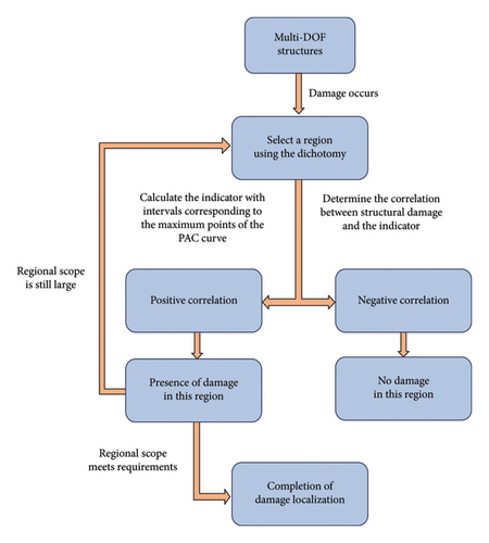
Unlike the conventional time series method, the MSM method selects data using the mutative-scale interval τ, as opposed to continuous intervals. Considering the stationary time series X = {x₁, x₂, …, x_N} and Y = {y₁, y₂, …, y_N−τ}, the time series Y is derived from X as Y(y_k = x_k+τ, k = 1, 2, …, N − τ). Here, N represents the length of the series X, which is substantially greater than τ and sufficiently extensive to ensure the validity of structural damage identification and localization. The interval τ specifically reflects the system’s properties [38]. Since the data are placed in a two-dimensional matrix, the joint occurrence entropy is then proposed as a corresponding two-dimensional entropy to help partition the original data, which makes the features of the signal better extracted. The procedural steps of the proposed methods are depicted in the flowchart presented in Figure 1. The damage localization methods incorporate an additional step beyond damage identification methods, which is elaborated in the subsequent introduction.

Details are in the caption following the image — **Figure 1**
Open in figure viewer PowerPoint

Flowchart of the proposed method.

2.1. VIRF

In this study, the series X = {x₁, x₂, …, x_N} represents the discrete VIRF at a specific sampling frequency. Differing from the impulse response function using an input impulse signal as excitation, VIRF can select any output responses to serve as the virtual excitation.

()

where F_zu(ω, i) is the frequency-response function, Z(ω, i) represents the Fourier transform of the structural vibration response z_i(t) at the MP i, and U(ω) denotes the Fourier transform of the excitation. Given that the Fourier transform U(ω) of the excitation is often unattainable in practical engineering applications, it becomes imperative to negate the influence of U(ω). Consequently the virtual frequency–response function F_zz(ω, i, j) is formulated as follows:

()

where Z(ω, j) is the Fourier transform of the virtual excitation z_j(t) at the RP j. This approach also reflects the intrinsic behavior of the structure, and F_zz(ω, i, j) has been demonstrated to be stable [39]. Consequently, the VIRF between z_j(t) and z_i(t), being the inverse Fourier transform of the virtual frequency–response function F_zz(ω, i, j), remains unaffected by the variations in excitation.

Acquiring and analyzing the VIRF constitute the initial step in the proposed study, ensuring that the collected acceleration signal solely reflects the characteristics of the structure. In damage identification methods, the selection of MP and RP can be arbitrary, but it is advisable to choose points distanced from each other, as this facilitates the belief that damage occurs between the two selected points. However, in damage localization methods, the selection of points becomes significantly more critical, as varying combinations of these points are utilized to ascertain the location of the damage.

2.2. Pearson Correlation Coefficient

To determine an appropriate τ for damage detection, the Pearson correlation function is utilized to investigate the impact of various τ values on the system. The Pearson correlation coefficient, which measures the linear relationship between two continuous variables, is defined as the quotient of the covariance and standard deviation between these variables [40], as delineated in the following equation:

()

where cov(X, Y) denotes the covariance of X and Y, and σ_X, σ_Y represent their respective standard deviations. E[X] signifies the mathematical expectation of X, and E[Y] signifies the mathematical expectation of Y. Generally, the Pearson correlation coefficient quantifies the correlation between variables X and Y, ranging from −1 to 1. For the given stationary time series X and Y defined before, the Pearson correlation function in equation (3) varies solely with τ, which means the Pearson correlation function C_X,Y here is a function of τ. Consequently, a new variable, C_τ, termed the Pearson autocorrelation coefficient (PAC), is utilized to depict the correlation of the same sequence with different starting points. To derive C_τ, C_X,Y values under adjacent damage states are subtracted, their absolute values are arranged in a row, and the largest row sum is calculated. In the subsequent verification results, it is observed that the extreme values of the proposed C_τ exhibit a high correlation with the structural damage state, thereby becoming crucial to damage identification. The specific details are elucidated in the following paragraphs.

The additional steps for damage localization are also based mainly on the PAC. The simulation and experimental results collectively indicate that if the damage is situated between the MP and the RP, the indicator associated with the τ corresponding to the maximum value of C_τ increases as the damage progresses; when the indicator is tied to the τ corresponding to the minimum value of C_τ, it decreases with increasing damage. Conversely, if the damage is not located between the MP and the RP, the indicator exhibits the opposite behavior. For unfamiliar structures, the MSM method can be employed for progressive damage localization utilizing a dichotomous approach. The approaching points are gradually selected as the MPs and RPs to ascertain if damage occurs between these points until the distance meets the standards. The procedural steps of the damage localization flowchart are presented in Figure 2. This dichotomous method can gradually reduce the range of possible damage at the fastest speed, and the minimum range is the distance between adjacent acceleration sensors. In this study, some critical points are selected to localize the predetermined damage as a validation of the proposed damage localization method.

2.3. STSA

STSA [41–43] represents a feature extraction method rooted in statistical analysis, capable of effectively extracting characteristic information from the original signal through rapid and straightforward computations. The implementation of symbolic time series analysis is depicted in Figure 3.

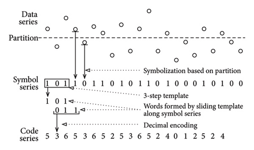
As shown in Figure 3, each generated partition is linked with a unique symbol, and the original time series data are mapped into the symbol space according to the partition they occupy. As a result, the raw time series is characterized by the corresponding series of symbols, and the code series is then computed by the binary algorithm, offering expanded possibilities for further exploration of the dynamical system [43]. The proposed MSM method retains this mode of symbolized data processing based on the new proposed joint occurrence entropy.

2.4. Joint Occurrence Entropy

Introduced by Shannon in 1948, Shannon’s entropy [44] measures the complexity and uncertainty of dynamic systems and also characterizes the statistical properties of symbol series. This metric helps to determine the partition number m, equivalently the number of rows and columns in the MSM. The classic expression of Shannon’s entropy for a given symbol series is formulated as follows:

()

where p_i represents the probability of a symbol occurring in the i^th partition, where i ranges from 1 to m. m signifies the number of partitions. In equation (4), a lower entropy typically indicates a more orderly system. Specifically, Shannon’s entropy reaches its minimum when p₁ = 1, p_i = 0(i ≠ 1) and attains its maximum when p₁ = p₂ = ⋯ = p_m [45].

In this study, the time series X is partitioned according to the maximum entropy principle, ensuring that the probability of data from series X is equally allocated to each partition. However, when the data from series Y are placed into these partitions, they should be as concentrated in one partition as possible corresponding to the minimum entropy. To solve this problem, the concept of joint occurrence entropy Q_m is proposed in equation (5) to offer quantitative statistics on the frequencies of various data within the matrix. The smaller the entropy value, the greater the probability of data at a specific location in the matrix, thereby more accurately reflecting the structure’s current state. Consequently, when Q_m reaches its minimum value, the corresponding m indicates the optimal number of partitions.

()

where p_ij represents the joint occurrence probability density of the symbols at the a_ij position in an m × m matrix, where i, j range from 1 to m; m denotes the number of partitions; and N is the length of the symbol series. Notably, an excessively large m can escalate computational costs; hence, an acceptable maximum value of m is 5 in this study, which is determined by analyzing the variations of Q_m with different m values.

2.5. MSM

The MSM is established to extract structural characteristics accurately with less amount of computation. Initially, the stationary time series X = {x₁, x₂, …, x_N} and Y = {y₁, y₂, …, y_N−τ} are discretized into m partitions following the maximum entropy principle, with each partition assigned a symbol from 1 to m. The probability density function of data from X in the i^th partition is represented by p_i and that of data from Y in the j^th partition by p_j, where i, j = 1, 2, …, m. For every possible pair of elements (x_k, y_k), the joint occurrence probability density that x_k and y_k, respectively, belong to the i^th and j^th partitions is given by p_ij. This forms the MSM A, with each entry comprising the joint occurrence probability density a_ij = p_ij. In addition, the joint occurrence probability density function is defined as

, and based on the maximum entropy principle,

()

It follows from this that the matrix A(τ) has the largest eigenvalue 1/m. The eigenvalues of matrix A(τ) can be denoted with Λ as

()

where 1/m = |λ₁| ≥ |λ₂| ≥ ⋯≥|λ_m|.

In this study, the second-largest eigenvalue D = |λ₂| has been selected as the damage detection indicator because of its particularity, which can be proved by QR iteration exploring the variation in A(τ) [46]. It is assumed that matrix A is diagonalizable such that U⁻¹AU = diag(λ₁, …, λ_m) with U = [u₁, …, u_m], and |λ₁| ≥ |λ₂| ≥ ⋯≥|λ_m|. A unit vector q⁽⁰⁾ is constructed to simulate the variation of A with τ.

()

There is nothing special about the choice of q^(τ), which is used only to discuss the properties of the matrix. If α₁ ≠ 0, then it follows that

()

Since q^(τ) ∈ span{A^τq⁽⁰⁾}, it can be concluded that

()

and furthermore,

()

where O represents an infinitesimal value. In the iterative process of the matrix, the eigenvalues λ₁ and λ₂ dictate the matrix’s convergence. Given that |λ₁| approximates 1/m, the matrix’s variation concerning τ is intrinsically linked to the second-largest eigenvalue λ₂ [47]. As is proved that it is able to reflect the characteristics of an iterative matrix by the above theoretical derivation, the second-largest eigenvalue is selected as the indicator for structural damage analysis. Furthermore, a large amount of simulation and experimental studies can demonstrate that the second-largest eigenvalue is an effective and reliable damage indicator that increases monotonically with escalating levels of damage severity with different damage types, and other eigenvalues do not have the same effect.

3. Numerical Studies

A simple 10-DOF model is constructed for damage identification and damage localization, which with its schematic is illustrated in Figure 4. The mass M, stiffness K, and damping ratio ζ for each DOF are set to 10 kg, 1200 N/m, and 0.05, respectively. Five damage scenarios are created by reducing the stiffness of the sixth DOF by 0, 10%, 20%, 30%, and 40% relative to its original stiffness. Random Gaussian white noise (20–150 Hz) acting as seismic excitation is applied at M 1. In addition, five independent trials are performed for each damage scenario to validate the simulation’s effectiveness. A total of 50 s of response data is sampled from each DOF at a sampling frequency of f_s = 100 Hz.

3.1. Damage Identification

3.1.1. Procedure

(1)
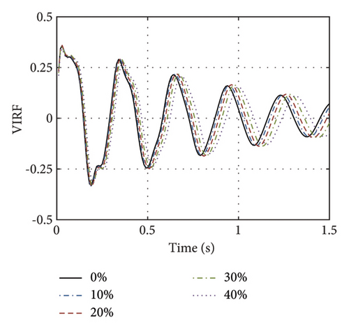
The acceleration response measured at the 1^st DOF serves as the virtual input to the structural frequency–response function, while the acceleration at the 10th DOF acts as the output, so the virtual frequency–response function of the structure F_zz(ω, 10, 1) is derived using the 1^st and 10^th DOF as the RP and MP (RP1 and MP10), respectively. Subsequently, the VIRF F(t) is determined via the inverse Fourier transform, and the mean value of the five trials is depicted in Figure 5(a), highlighting the first 3 s, where the attenuation is notably significant. The Figure 5(a) clearly shows that as the stiffness decreases, the attenuation of VIRF curves progressively slows down, which indicates that VIRF curves can effectively represent the severity of structural damage.
(2)
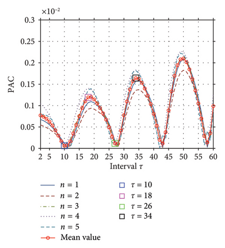
The correlation between PAC C_τ and the interval τ is analyzed and illustrated in Figure 5(b), where five gray curves represent the outcomes of five independent trials, and the average is depicted in red. It is observed that the extreme points on the curves are relatively concentrated at some specific points and alternate regularly, which means the trend of the curve follows a certain periodic law. Starting at the first minimum point, four points are selected to investigate whether the corresponding τ is the suitable interval for reflecting the structural damage condition. Ultimately, Intervals 10 and 26, corresponding to the minimum extreme values, and Intervals 18 and 34, corresponding to the maximum extreme values, are sequentially chosen to validate the method’s effectiveness. In theory, the PAC curves of a structure usually show a cyclical trend, and the choices of extreme values are arbitrary under the principle that N is substantially greater than τ. However, if a structure’s PAC curve does not exhibit a perfect cyclical trend due to factors such as environmental interference, there is still a high probability that the structural characteristic changes can be explored at the relatively concentrated extreme points on this PAC curve.
(3)
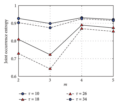
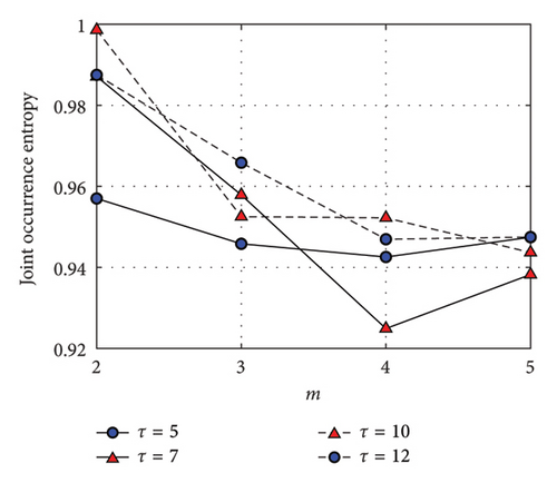
The VIRF F(t) undergoes partitioning and symbolization, guided by the joint occurrence entropy Q_m. Intervals 10, 18, 26, and 34 are integrated into Q_m curves plotted against m, as illustrated in Figure 6. The entropy curves for these four intervals reach their minimum values when the number of partitions m equals 3, indicating that this is the optimal partition number.
(4)
Partition number 3 selected above is also the row number and column number of the MSM. Subsequently, a 3 × 3 matrix A(τ) is constructed as
()

The damage indicator D is the second-largest eigenvalue of matrix A, D = |λ₂|. The identification of the structural damage can be realized by comparing damage indicators under different damage conditions.

3.1.2. Results

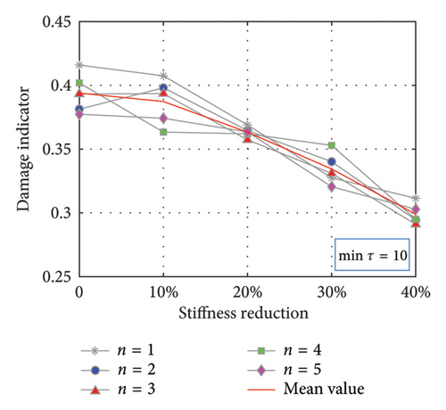
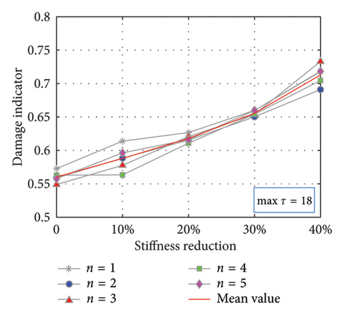
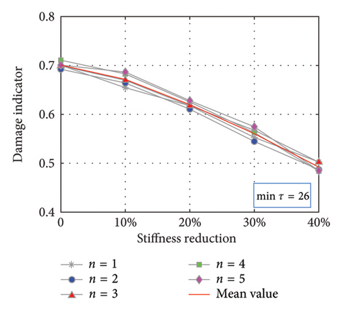
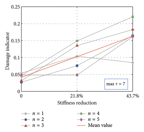
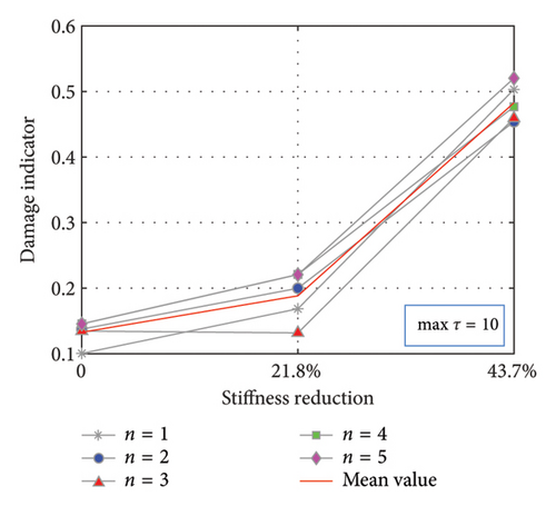
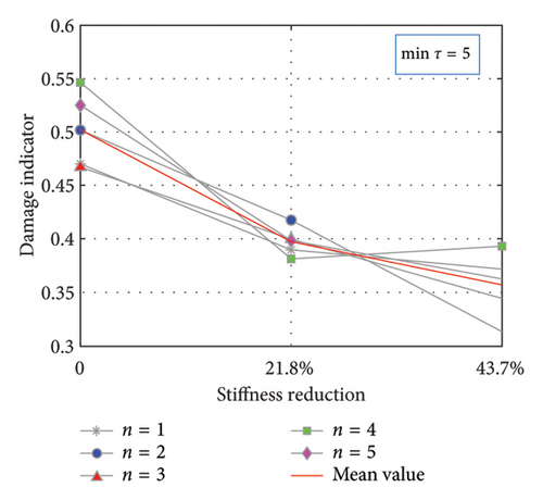
Figure 7 illustrates the correlation between the severity of damage and the damage indicator D, where the five gray curves represent the outcomes of five independent simulations, with their mean value shown in red. Figures 7(b) and 7(d), featuring Intervals of 18 and 34, correspond to the maximum extreme points on the C_τ curves. As the damage severity increases, the curves demonstrate a continuous upward trend. Conversely, Figures 7(a) and 7(c), with Intervals of 10 and 26 corresponding to the minimum extreme points on the C_τ curves, exhibit a downward trend. Therefore, when damage is present between the RP and MP, a positive correlation emerges between the damage indicator and the extent of damage, with intervals corresponding to the maximum extreme points on the C_τ curves. In addition, the damage indicator curves under 5 different excitations display mild fluctuations in some instances, suggesting the robustness of the damage identification method against variations in excitation.

3.2. Damage Localization

The same 10-DOF model, as described in the above section, is utilized for the numerical analysis of damage localization.

3.2.1. Principle

The pivotal step in damage localization is selecting the MP and RP of the structure, where different choices for RP and MP result in contrasting behaviors of the C_τ curves. The fundamental principle of damage localization is that if damage occurs between the RP and MP, and the intervals τ correspond to the maximum extreme points on the C_τ curves, the indicator rises with worsening damage and declines when the intervals correspond to the minimum extreme points. Conversely, if the damage is not present between the RP and MP, and the intervals correspond to the maximum extreme points on the C_τ curves, the damage indicator exhibits a negative correlation with damage severity, whereas a positive correlation is observed when the intervals correspond to the minimum extreme points.

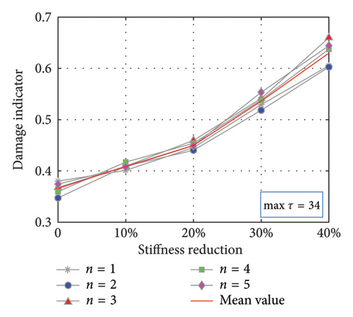
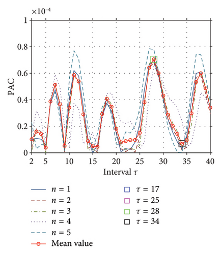
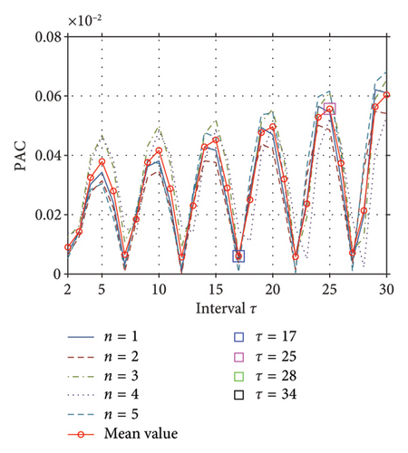
To validate the damage localization method, the critical points DOF5 and DOF7 are, respectively, selected to be the RPs as the control group, and the 10^th DOF is always the MP, and the results are compared together. The subsequent steps mirror those outlined in the previous section and the repetition is omitted. The Pearson correlation coefficient C_τ as a function of τ is illustrated in Figure 8. For the condition of RP5 and MP10 in Figure 8(a) that the damage occurs still between the RP and MP, the Maximum point 28 and the Minimum point 35 are arbitrarily chosen; on the contrary for RP7 and MP10 in Figure 8(b), the Maximum point 25 and the Minimum point 17 are selected. It is observed that the trend of the curves still presents a certain periodic law, in which every extreme point theoretically works. The partition number is still 3 and the second-largest eigenvalue D continues to serve as the indicator.

3.2.2. Results

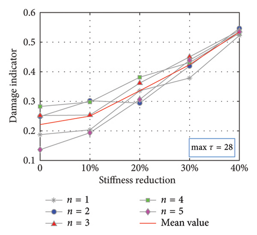
The results are depicted in Figure 9. As observed in Figures 9(a) and 9(b) for RP5 and MP10, when the C_τ curve reaches the maximum extreme points at Interval 28, the damage indicator escalates monotonically with increasing damage severity, in contrast to the behavior at Interval 34 corresponding to the minimum extreme point. Therefore, it is deduced that the damage occurred between the 5^th and 10^th DOFs. The opposite happens in Figures 9(c) and 9(d) for RP7 and MP10, where Interval 17 represents the minimum point on the C_τ curves, where the damage indicator rises with increasing damage severity. At the interval of 25 corresponding to the maximum point, the trend is reversed, which indicates that there is no damage present between the 7^th DOF and 10^th DOF. Consequently, combining this with the results of the RP7 and MP10 cases, it can be deduced that the damage is likely near the 6^th DOF.

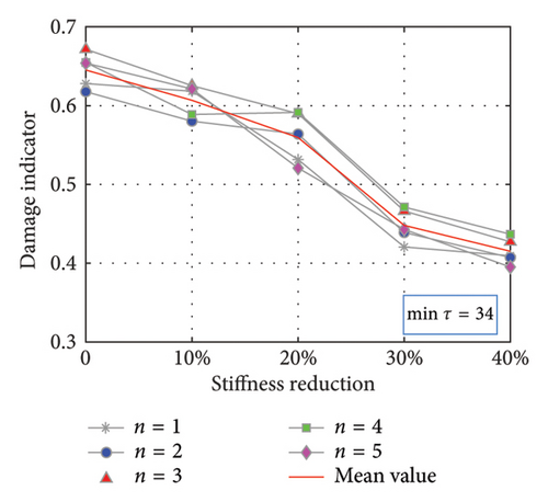
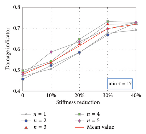
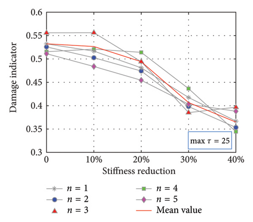
4. Experiment Validation

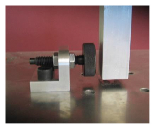
The experimental model used for damage identification and localization is a testbed structure located at the Los Alamos National Laboratory [48], as illustrated in Figure 10(a). An adjustable bumper mounted on the second floor is enlarged in Figure 10(b). This model is a 4-DOF structure (with the base as the 1^st DOF) comprising aluminum columns and plates with bolted joints. Each floor is interconnected by an aluminum plate (30.5 × 30.5 × 2.5 cm), supported by four aluminum columns (17.7 × 2.5 × 0.6 cm). Notably, the structure is designed to slide only in the x-direction, as can be observed in Figure 10(c).

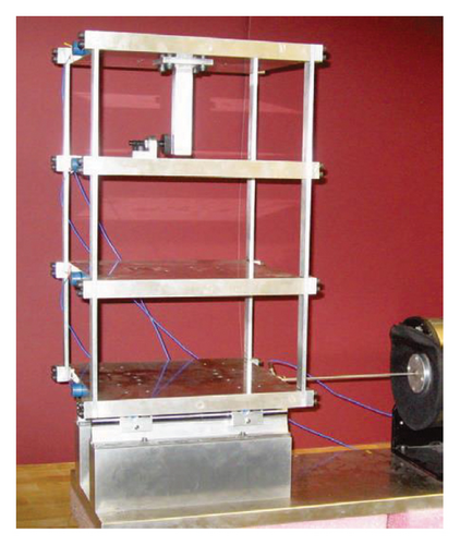
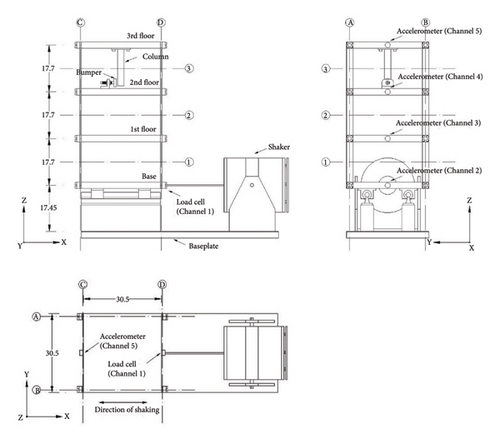
There are 17 structural states in the experiment, eight of which are utilized to validate the proposed method with damage caused by stiffness reduction and nonlinearity, as outlined in Table 1. In addition, band-limited random excitation ranging from 20 to 150 Hz is used to provide lateral excitation to the structure, and four accelerometers are mounted on each DOF to capture the structure’s acceleration responses, and the signal’s sampling frequency is set at 320 Hz, resulting in time histories covering 25.6 s.

Table 1. The structural state conditions.

State	Damage condition	Description
1	Undamaged	Baseline
4	Stiffness reduction 87.5% in column 1BD	21.8% equivalent stiffness reduction between DOF1 and DOF2
5	Stiffness reduction 87.5% in column 1AD and 1BD	43.7% equivalent stiffness reduction between DOF1 and DOF2
10	Gap (0.20 mm)	Nonlinear damage at DOF3 (the lowest level of damage severity)
11	Gap (0.15 mm)	Nonlinear damage at DOF3
12	Gap (0.13 mm)	Nonlinear damage at DOF3
13	Gap (0.10 mm)	Nonlinear damage at DOF3
14	Gap (0.05 mm)	Nonlinear damage at DOF3 (the highest level of damage severity)

4.1. Experimental Results of Stiffness Reduction States

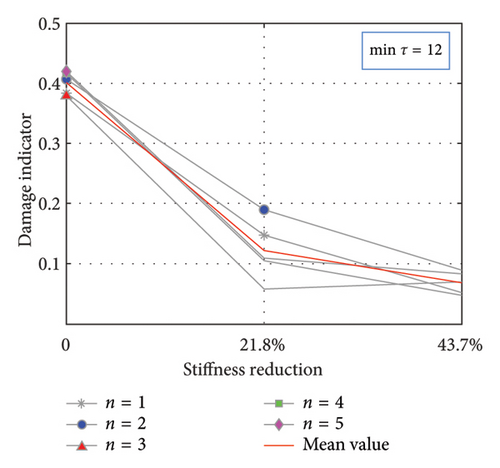
The damage caused by stiffness reduction is studied for damage identification with 3 damage cases as described in the Table 1 (State 1, State 4, and State 5). The acceleration responses of the 1^st and 4^th DOFs are chosen as the virtual excitation and output for damage identification (RP1 and MP4). Approximately 50 sets of independent data are available for each damage case, with 5 randomly selected from five separate trials to ascertain the effectiveness and robustness of the proposed method.

4.1.1. Damage Identification

First, the VIRF is depicted in Figure 11(a), and it is observed that the damage affects the attenuation of signals so that the damage identification is still reliable. Second, the PAC curves are generated in Figure 11(b). From the Figure 11(b), it is summarized that the low sampling frequency used in the test may lead to coordinate deviations of τ, namely, the abscissas of the extreme points may occur between two adjacent integers. Under this premise, it is proven that the damage condition can be better reflected at Intervals 5,7,10, and 12, which are taken as references to verify the damage identification for the structure. Third, the partition and symbolization based on the joint occurrence entropy are plotted in Figure 12 based on minimum and maximum intervals, respectively. Particularly, the partition number is set to 4 because the entropy Q_m is minimum at m = 4 for Intervals 7 and 12, while the entropy does not change significantly for Intervals 5 and 10 when m ≥ 3. Subsequently, the MSM is derived as

()

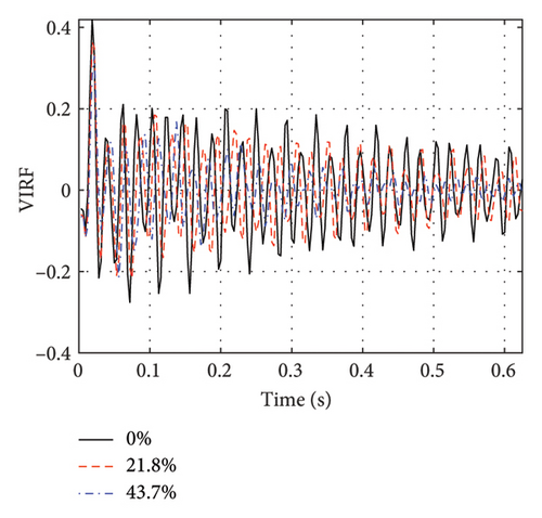
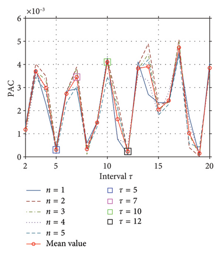
The damage indicator D, identified as the second-largest eigenvalue of the matrix, and its variation with damage severity for different extreme points are depicted in Figure 13. Essentially, the experimental results concerning the variation trend of the damage indicator for both maximum and minimum intervals align with the aforementioned numerical results, thereby corroborating the effectiveness of the proposed method for damage identification.

4.1.2. Damage Localization

For damage localization, the 2^nd and 4^th DOFs are chosen as the RP and MP (RP2 and MP4), respectively, to verify that the damage did not occur between them. In contrast, the choice of RP1 and MP2 was also explored. The operation procedure and parameter selection are the same as the damage identification (RP1 and MP4), and the data of a maximum point of the PAC curve were chosen to compare the results, as shown in Figure 14.

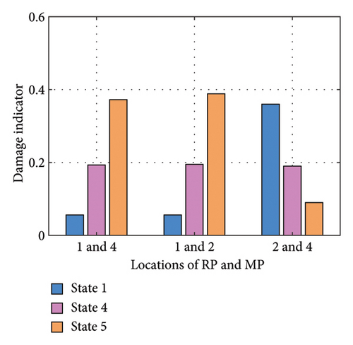
It can be intuitively seen from the bar chart that for RP1 and MP2 and RP2 and MP4, the damage indicators develop opposite with the increase of damage, but there is not much difference between the conditions RP1 and MP2 and RP1 and MP4, which verifies that the damage occurs between DOF1 and DOF2.

In addition, it can be inferred from several other choices of RP and MP that the sensitivity of the damage indicators is heightened when the damage is located between the RP and MP, leading to measured results that are less prone to interference. When the damage is not situated between and is distant from the RP and MP, errors are more likely to occur in the identification and localization of the damage.

4.1.3. Comparison With the WPT Method

Also, as a dimensionality reduction approach in damage identification, the WPT method is employed to facilitate a comparison with the proposed method, and the related conclusions have been drawn by Li and Li [25]. The average values from multiple calculations of the MSM indicator with RP1 and MP2 as well as RP1 and MP4 are displayed together. For a more intuitive comparison, the values from the three damage states collectively subtract the non-damaged state values, and the mean values of the damage indicators are normalized (the value of the non-damaged state is 0 and the value of the max-damaged state is 1), as illustrated in Figure 15(a). Similar procedures are applied to the WPT results, as depicted in Figure 15(b).

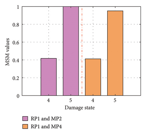
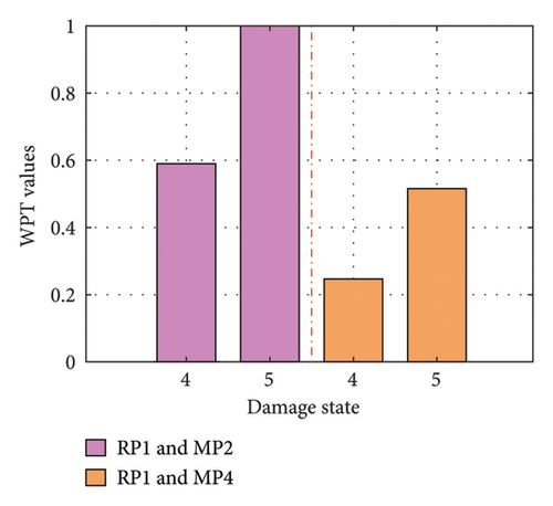
In damage identification, when the RP is RP1 and the MP shifts from MP2 to MP4, the MSM damage indicator remains relatively stable as the MP moves farther from the damage site. In contrast, the damage indicator for the WPT method noticeably decreases, leading to increased errors. Consequently, the proposed method demonstrates greater robustness in the selection of RP and MP locations.

In the context of damage localization, the WPT method relies on comparing the indicator values of different RP and MP; as in the example above, when the RP is fixed, the closer proximity between the damage and MP correlates with a higher damage indicator value. Therefore, the WPT method for damage localization demands extensive calculations, especially for complex structures, and is susceptible to error interference. In contrast, the proposed damage localization method offers better flexibility, as it provides more precise directivity in exploring the damage location.

4.2. Experimental Results of Nonlinear Damage States

The nonlinear damage is caused by the bumper in Figure 10(b). When the column contacts the bumper mounted on the second floor, damage can be simulated by inducing nonlinear behavior. The position of the bumper can be adjusted to vary the extent of impact that occurs at a particular excitation level to form 5 damage states (States 10–14) as outlined in Table 1, where the largest gap (0.20 mm) represents the lowest level of damage severity.

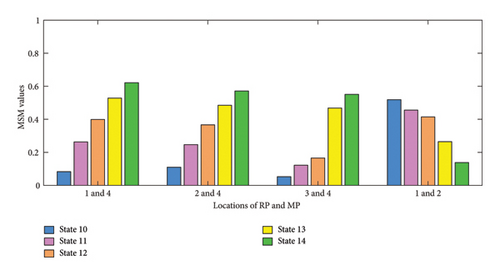
The proposed MSM method is also applicable in the cases of nonlinear damage, and the procedure of damage detection is the same as that of stiffness reduction cases. We select the locations of 4 RPs and MPs that are RP1 and MP4, RP2 and MP4, RP3 and MP4, and RP1 and MP2 as shown in Figure 16(a). The mean values of the indicators are then plotted with the intervals corresponding to the maximum points in the PAC in a bar chart. For the first three conditions, the damage indicators all increase gradually with the damage growth, but for the condition RP1 and MP2, the bar chart shows the opposite trend. Considering the above conditions, the damage may occur between DOF3 and DOF4.

4.2.1. Comparison With the RRC Method

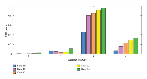
As a damage identification and localization method for damage identification extracting damage-sensitive features from time series models, the damage index residual reliability criterion (RRC) proposed by Entezami [17] was also verified to be reliable with nonlinear damage states in the same laboratory model. This method selected the signal from the accelerator sensors on each DOF for processing and drew a bar graph for all the cases as shown in Figure 16(b). The damage index RRC from DOF3 nearing the damage was significantly larger than other DOFs and increased with the deepening of the damage. However, except for DOF4, the development of damage could not be recognized at other DOFs.

In contrast, no significant attenuation of MSM values is observed with multiple locations of RP and MP which reflects the robustness of the MSM method in damage detection of multifreedom structures. In other words, when applied to a structure that has more degrees of freedom and the possible location of the damage is unknown, the effectiveness of the damage detection method will not deteriorate due to the different choices of signal channels. This allows for faster detection of damage occurrence and progression.

At the same time, MSM values for damage localization are also proven effective. While other methods still rely on comparing data from different locations, the method proposed can lock the scope of damage faster and use dichotomy to reduce this scope; the minimum scope is the distance between adjacent sensors. For example, damage localization on a 5-DOF structure (damage is between DOF4 and DOF5) by their method may need 5 times of calculation to process the signal of each DOF for comparison, while the MSM method only needs, RP1 and MP3 and RP3 and MP4, two steps to lock the location, thereby greatly improving the efficiency of calculation. These two ways can all realize damage localization effectively and will have different application values.

4.3. Computational Efficiency

In addition to the accuracy and robustness of damage detection, this method is also advanced in computational efficiency. Compared to the conventional STSA method [43], it can save more time in calculation because of the application of intermittent points and matrices. We use the stopwatch timer in MATLAB to calculate the time from the start to the indicator calculation of the two algorithms under the three models in Table 2, and the average of the five trials is taken. It can be seen from the Table 2 that for any model, the running time of the proposed method has a certain reduction compared to conventional STSA, which means that in the application of large structures with many DOFs, computing efficiency will be improved significantly.

Table 2. Comparisons of the computation time.

Model	Damage type	Computation time (s)
Model	Damage type	STSA	MSM
Simulation	Stiffness reduction	2.4673	1.5013
Experiment	Stiffness reduction	3.2822	1.9408
Experiment	Nonliner damage	3.7500	2.0917

5. Conclusions and Discussion

5.1. Conclusions

Time series–based methods for damage identification and localization consistently encounter challenges in the effective and efficient processing of the data in SHM. To address these issues, this study introduces a MSM method, offering an information-rich representation of the overall structural vibration performance for characterizing damage and establishing a reliable damage indicator: the matrix’s second-largest eigenvalue. Along with the corresponding joint occurrence entropy, the proposed MSM efficiently extracts valuable information from complex data with high accuracy.

In the process of MSM, the VIRF is initially employed to mitigate the effects of varying excitations. Subsequently, suitable intervals are selected based on the PAC C_τ, which is derived from the Pearson correlation coefficient, to construct the MSM. Concurrently, joint occurrence entropy, grounded in Shannon’s entropy, is introduced to analyze one-dimensional time series data within a two-dimensional matrix, significantly enhancing the efficiency of the calculations.

In damage localization, the flexibility in selecting MPs and RPs facilitates pinpointing the potential scope of damage and ultimately achieving damage localization by progressively narrowing the scope. In this paper, a detailed flowchart is given for damage location procedures of general structures. Both a 10-DOF numerical model subjected to random Gaussian white noise and a 4-DOF testbed structure under varying excitations have been employed to validate the method. Compared to WPT and RCC values, it is demonstrated that the innovative damage indicator is highly responsive to varying degrees of damage and is not significantly influenced by the choice of MP and RP, affirming that the refined method is more efficient and robust. The MSM method also shows advantages in comparison with the conventional method in computational efficiency.

In conclusion, the proposed method for damage identification and localization offers more precise damage detection outcomes with reduced computational effort. It possesses significant advantages in evaluating the degree of damage and ascertaining its extent, proving to be highly valuable for practical structural applications.

5.2. Limitations and Prospects

Due to the inherent limitation of the theory of VIRF, the research in this paper only considers single-point type random excitation, including the dependent ambient excitation. More validation of the MSM method on in-service structures is currently in progress.

At present, the proposed damage localization method can be applied to the one-dimensional structure that can be simplified into a chain model such as frame structures, long-span bridges, and high-level structures. For more complex spatial structures, some more complicated operations are required which will be shared in subsequent studies.

Conflicts of Interest

The authors declare no conflicts of interest.

Funding

This work was supported by the National Natural Science Foundation of China (Grant no. 52078284), the GuangDong Basic and Applied Basic Research Foundation (Grant nos. 2024A1515010090 and STKJ2023067), the Guangdong Provincial University Innovation Team Project (Grant no. 2020KCXTD012), and the Open Projects Foundation (Grant no. BHSKL20-10-KF) of the State Key Laboratory for Health and Safety of Bridge Structures. Their financial support is gratefully acknowledged. In addition, the authors would like to thank Jiezhong Huang for the invaluable guidance and support in managing the funding provided by the National Natural Science Foundation of China (Grant no. 52308318) and Tao Jiang for GuangDong Basic and Applied Basic Research Foundation (Grant no. 2022A1515010812).

Open Research

Data Availability Statement

The data are available from the corresponding author on reasonable request.

References

1 Avci O., Abdeljaber O., Kiranyaz S., Hussein M., Gabbouj M., and Inman D. J., A Review of Vibration-Based Damage Detection in Civil Structures: From Traditional Methods to Machine Learning and Deep Learning Applications, Mechanical Systems and Signal Processing. (2021) 147, https://doi.org/10.1016/j.ymssp.2020.107077.
10.1016/j.ymssp.2020.107077
Web of Science® Google Scholar
2 Hou R. and Xia Y., Review on the New Development of Vibration-Based Damage Identification for Civil Engineering Structures: 2010–2019, Journal of Sound and Vibration. (2021) 491, https://doi.org/10.1016/j.jsv.2020.115741.
10.1016/j.jsv.2020.115741
Web of Science® Google Scholar
3 Fan W. and Qiao P., Vibration-Based Damage Identification Methods: A Review and Comparative Study, Structural Health Monitoring. (2011) 10, no. 1, 83–111, https://doi.org/10.1177/1475921710365419, 2-s2.0-79751492551.
10.1177/1475921710365419
Web of Science® Google Scholar
4 Deng Z., Huang M., Wan N., and Zhang J., The Current Development of Structural Health Monitoring for Bridges: A Review, Buildings. (2023) 13, no. 6, https://doi.org/10.3390/buildings13061360.
10.3390/buildings13061360
Web of Science® Google Scholar
5 Farrar C. and Worden K., Structural Health Monitoring: A Machine Learning Perspective, 2013, John Wiley and Sons, Ltd, West Sussex, UK.
Google Scholar
6 Xia Z., Li A., Li J., Shi H., Duan M., and Zhou G., Model Updating of an Existing Bridge With High-Dimensional Variables Using Modified Particle Swarm Optimization and Ambient Excitation Data, Measurement. (2020) 159, https://doi.org/10.1016/j.measurement.2020.107754.
10.1016/j.measurement.2020.107754
Web of Science® Google Scholar
7 Yuen K., Beck J., and Katafygiotis L., Efficient Model Updating and Health Monitoring Methodology Using Incomplete Modal Data Without Mode Matching, Structural Control and Health Monitoring. (2006) 13, no. 1, 91–107, https://doi.org/10.1002/stc.144, 2-s2.0-33144461314.
10.1002/stc.144
Web of Science® Google Scholar
8 Zhang J., Huang M., Wan N., Deng Z., He Z., and Luo J., Missing Measurement Data Recovery Methods in Structural Health Monitoring: The State, Challenges and Case Study, Measurement. (2024) 231, https://doi.org/10.1016/j.measurement.2024.114528.
10.1016/j.measurement.2024.114528
Web of Science® Google Scholar
9 Peng Z., Li J., and Hao H., Data Driven Structural Damage Assessment Using Phase Space Embedding and Koopman Operator Under Stochastic Excitations, Engineering Structures. (2022) 255, https://doi.org/10.1016/j.engstruct.2022.113906.
10.1016/j.engstruct.2022.113906
Web of Science® Google Scholar
10 Entezami A., Shariatmadar H., and Mariani S., Early Damage Assessment in Large-Scale Structures by Innovative Statistical Pattern Recognition Methods Based on Time Series Modeling and Novelty Detection, Advances in Engineering Software. (2020) 150, https://doi.org/10.1016/j.advengsoft.2020.102923.
10.1016/j.advengsoft.2020.102923
Web of Science® Google Scholar
11 Heravi M. A., Tavakkoli S. M., and Entezami A., Structural Health Monitoring by Probability Density Function of Autoregressive-Based Damage Features and Fast Distance Correlation Method, Journal of Vibration and Control. (2022) 28, no. 19-20, 2786–2802, https://doi.org/10.1177/10775463211020198.
10.1177/10775463211020198
Web of Science® Google Scholar
12 Huang M., Ling Z., Sun C. et al., Two-Stage Damage Identification for Bridge Bearings Based on Sailfish Optimization and Element Relative Modal Strain Energy, Structural Engineering & Mechanics. (2023) 86, no. 6, 715–730, https://doi.org/10.12989/sem.2023.86.6.715.
10.12989/sem.2023.86.6.715
Web of Science® Google Scholar
13 Huang M., Zhang J., Li J., Deng Z., and Luo J., Damage Identification of Steel Bridge Based on Data Augmentation and Adaptive Optimization Neural Network, Structural Health Monitoring. (2024) https://doi.org/10.1177/14759217241255042.
10.1177/14759217241255042
Web of Science® Google Scholar
14 Alves V. and Cury A., A Fast and Efficient Feature Extraction Methodology for Structural Damage Localization Based on Raw Acceleration Measurements, Structural Control and Health Monitoring. (2021) 28, no. 7, https://doi.org/10.1002/stc.2748.
10.1002/stc.2748
PubMed Web of Science® Google Scholar
15 Huang M., Zhang J., Hu J., Ye Z., Deng Z., and Wan N., Nonlinear Modeling of Temperature-Induced Bearing Displacement of Long-Span Single-Pier Rigid Frame Bridge Based on DCNN-LSTM, Case Studies in Thermal Engineering. (2024) 53, https://doi.org/10.1016/j.csite.2023.103897.
10.1016/j.csite.2023.103897
Web of Science® Google Scholar
16 Bastanlar Y. and Orhan S., M. A. A. Fernandez and C. M. Travieso-Gonzalez, Self-Supervised Contrastive Representation Learning in Computer Vision, Artificial Intelligence Annual Volume 2022, 2022, IntechOpen, Rijeka, Croatia.
10.5772/intechopen.104785
Google Scholar
17 Entezami A. and Shariatmadar H., An Unsupervised Learning Approach by Novel Damage Indices in Structural Health Monitoring for Damage Localization and Quantification, Structural Health Monitoring. (2018) 17, no. 2, 325–345, https://doi.org/10.1177/1475921717693572, 2-s2.0-85040048191.
10.1177/1475921717693572
Web of Science® Google Scholar
18 Entezami A., Sarmadi H., Salar M., De Michele C., and Arslan A. N., A Novel Data-Driven Method for Structural Health Monitoring Under Ambient Vibration and High-Dimensional Features by Robust Multidimensional Scaling, Structural Health Monitoring. (2021) 20, no. 5, 2758–2777, https://doi.org/10.1177/1475921720973953.
10.1177/1475921720973953
Web of Science® Google Scholar
19 Entezami A., Sarmadi H., and Behkamal B., A Novel Double-Hybrid Learning Method for Modal Frequency-Based Damage Assessment of Bridge Structures Under Different Environmental Variation Patterns, Mechanical Systems and Signal Processing. (2023) 201, https://doi.org/10.1016/j.ymssp.2023.110676.
10.1016/j.ymssp.2023.110676
Web of Science® Google Scholar
20 Sarmadi H., Entezami A., and De Michele C., Probabilistic Data Self-Clustering Based on Semi-Parametric Extreme Value Theory for Structural Health Monitoring, Mechanical Systems and Signal Processing. (2023) 187, https://doi.org/10.1016/j.ymssp.2022.109976.
10.1016/j.ymssp.2022.109976
Web of Science® Google Scholar
21 Jiang X. and Mahadevan S., Wavelet Spectrum Analysis Approach to Model Validation of Dynamic Systems, Mechanical Systems and Signal Processing. (2011) 25, no. 2, 575–590, https://doi.org/10.1016/j.ymssp.2010.05.012, 2-s2.0-78649538519.
10.1016/j.ymssp.2010.05.012
Web of Science® Google Scholar
22 Xie D. and Tang H., Application of Wavelet Packet Transform and Neural Network to Detect Damage of Elastic Thin Plate, Advanced Materials Research. (2012) 594–597.
Google Scholar
23 Xu Q., Damage Identification Investigation of Retaining Wall Structures Based on a Virtual Impulse Response Function, Shock and Vibration. (2016) 2016, 1–13, https://doi.org/10.1155/2016/1346939, 2-s2.0-84985919255.
10.1155/2016/1346939
Web of Science® Google Scholar
24 Qu C., Yi T., and Li H., Mode Identification by Eigensystem Realization Algorithm Through Virtual Frequency Response Function, Structural Control and Health Monitoring. (2019) 26, no. 10, https://doi.org/10.1002/stc.2429, 2-s2.0-85069919372.
10.1002/stc.2429
PubMed Web of Science® Google Scholar
25 Li Q. and Li D., Structure Damage Identification Under Ambient Excitation Based on Wavelet Packet Analysis, Journal of Physics: Conference Series. (2017) 842, no. 1, https://doi.org/10.1088/1742-6596/842/1/012023, 2-s2.0-85021206318.
10.1088/1742-6596/842/1/012023
Google Scholar
26 Arroyo D., Latorre R., Varona P., and Rodriguez F. B., Application of Symbolic Dynamics to Characterize Coordinated Activity in the Context of Biological Neural Networks, Journal of the Franklin Institute. (2013) 350, no. 10, 2967–2981, https://doi.org/10.1016/j.jfranklin.2013.03.018, 2-s2.0-84887320718.
10.1016/j.jfranklin.2013.03.018
Web of Science® Google Scholar
27 Cammarota C. and Rogora E., Independence and Symbolic Independence of Nonstationary Heartbeat Series during Atrial Fibrillation, Physica A: Statistical Mechanics and its Applications. (2005) 353, 323–335, https://doi.org/10.1016/j.physa.2005.01.030, 2-s2.0-18844416137.
10.1016/j.physa.2005.01.030
Web of Science® Google Scholar
28 Xu M. and Xi D., Multi-Scale Analysis of Stock Volatility Based on Symbolic Time Series Method, Journal of Wuhan University of Technology. (2013) 35, 595–598, https://doi.org/10.3963/j.issn.2095-3852.2013.04.032.
10.3963/j.issn.2095-3852.2013.04.032
Google Scholar
29 Wu J., Meng Y., and Gao Y., Multi-Scale Symbolic Analysis of Instantaneous Velocity Time Series in the Static Mixer With Twisted-Leaves, Journal of Basic Science and Engineering. (2011) 19, 799–809, https://doi.org/10.3969/j.issn.1005-0930.2011.05.013, 2-s2.0-81555210063.
10.3969/j.issn.1005-0930.2011.05.013
Google Scholar
30 Daw C. S., Finney C. E. A., Nguyen K., and Halow J. S., Symbol Statistics: A New Tool for Understanding Multiphase Flow Phenomena, Heat Transfer: Volume 5-Numerical and Experimental Methods in Heat Transfer. ASME International Mechanical Engineering Congress and Exposition, 1998, 221–229.
Google Scholar
31 Hu S., Qian Y., and Yan R., Anomaly Detection Using Symbolic Time Series Analysis Based on Probability Density Space Partitioning, Journal of Vibration Engineering. (2014) 27, 780–784, https://doi.org/10.3969/j.issn.1004-4523.2014.05.019.
10.3969/j.issn.1004-4523.2014.05.019
Google Scholar
32 Ly A., Marsman M., and Wagenmakers E. J., Analytic Posteriors for Pearson’s Correlation Coefficient, Statistica Neerlandica. (2018) 72, no. 1, 4–13, https://doi.org/10.1111/stan.12111, 2-s2.0-85021828747.
10.1111/stan.12111
PubMed Web of Science® Google Scholar
33 Fisher R., Frequency Distribution of the Values of the Correlation Coefficient in Samples From an Indefinitely Large Population, Biometrika. (1915) 10, no. 4, 507–521, https://doi.org/10.2307/2331838.
10.2307/2331838
CAS Google Scholar
34 Fisher R., A Mathematical Examination of the Methods of Determining the Accuracy of Observation by the Mean Error, and by the Mean Square Error, Monthly Notices of the Royal Astronomical Society. (1920) 80, no. 8, 758–770, https://doi.org/10.1093/mnras/80.8.758.
10.1093/mnras/80.8.758
Google Scholar
35 Fisher R., On the “Probable Error” of a Coefficient of Correlation Deduced From a Small Sample, Metron. (1921) 1, 3–32.
Google Scholar
36 Fisher R., On the Mathematical Foundations of Theoretical Statistics, Springer Series in Statistics. (1992) 222, 11–44, https://doi.org/10.1007/978-1-4612-0919-5_2.
10.1007/978-1-4612-0919-5_2
Google Scholar
37 Liu X. and Tse C. K., A Complex Network Perspective of World Stock Markets: Synchronization and Volatility, International Journal of Bifurcation and Chaos. (2012) 22, no. 06, https://doi.org/10.1142/S0218127412501428, 2-s2.0-84863834869.
10.1142/S0218127412501428
Web of Science® Google Scholar
38 Yuan Q., Semba S., Zhang J., Weng T., Gu C., and Yang H., Multi-Scale Transition Matrix Approach to Time Series, Physica A: Statistical Mechanics and its Applications. (2021) 578, https://doi.org/10.1016/j.physa.2021.126116.
10.1016/j.physa.2021.126116
Web of Science® Google Scholar
39 Qu C., Yi T., and Li H., Modal Identification for Superstructure Using Virtual Impulse Response, Advances in Structural Engineering. (2019) 22, no. 16, 3503–3511, https://doi.org/10.1177/1369433219862951, 2-s2.0-85069505754.
10.1177/1369433219862951
Web of Science® Google Scholar
40 Schober P., Boer C., and Schwarte L. A., Correlation Coefficients: Appropriate Use and Interpretation, Anesthesia & Analgesia. (2018) 126, no. 5, 1763–1768, https://doi.org/10.1213/ANE.0000000000002864, 2-s2.0-85048115048.
10.1213/ANE.0000000000002864
PubMed Web of Science® Google Scholar
41 Xiang K. and Jiang J., Study on Symbolization Analysis of Time Series, Pattern Recognition and Artificial Intelligence. (2007) 20, 154–161, https://doi.org/10.3969/j.issn.1003-6059.2007.02.003.
10.3969/j.issn.1003-6059.2007.02.003
Google Scholar
42 Jin N. and Li W., Study on the Analysis Method of Nonlinear Symbolic Time Series, Journal of Dynamics and Control. (2004) 2, 54–59, https://doi.org/10.3969/j.issn.1672-6553.2004.03.011.
10.3969/j.issn.1672-6553.2004.03.011
Google Scholar
43 Daw C. S., Finney C. E. A., and Kennel M. B., Symbolic Approach for Measuring Temporal Irreversibility, Physical Review E. (2000) 62, no. 2, 1912–1921, https://doi.org/10.1103/PhysRevE.62.1912.
10.1103/PhysRevE.62.1912
CAS PubMed Web of Science® Google Scholar
44 Shannon C., A Mathematical Theory of Communication, Bell System Technical Journal. (1948) 27, no. 3, 379–423, https://doi.org/10.1002/j.1538-7305.1948.tb01338.x, 2-s2.0-84940644968.
10.1002/j.1538-7305.1948.tb01338.x
Web of Science® Google Scholar
45 Presse S., Ghosh K., Lee J., and Dill K. A., Principles of Maximum Entropy and Maximum Caliber in Statistical Physics, Reviews of Modern Physics. (2013) 85, no. 3, 1115–1141, https://doi.org/10.1103/RevModPhys.85.1115, 2-s2.0-84882279791.
10.1103/RevModPhys.85.1115
CAS Web of Science® Google Scholar
46 Golub G. H. and Van Loan C. F., Matrix Computations, 1996, 3rd edition, The Johns Hopkins University, Baltimore.
CAS Web of Science® Google Scholar
47 Zhang C. and Berry R., Time Autocorrelation Function Analysis of Master Equation and Its Application to Atomic Clusters, The Journal of Chemical Physics. (2005) 123, no. 9, https://doi.org/10.1063/1.2000243, 2-s2.0-33646398062.
10.1063/1.2000243
Web of Science® Google Scholar
48 Figueiredo E. and Flynn E., Structural Health Monitoring Algorithm Comparisons Using Standard Data Sets, 2009, Los Alamos National Lab.(LANL), Los Alamos, Technical Report.
Google Scholar

All articles

Identification and Localization of Structural Damage Using the Second-Largest Eigenvalue of the Mutative-Scale Symbolic Matrix as the Damage Indicator

Abstract

1. Introduction