Structural Control and Health Monitoring

Volume 2025, Issue 1 1806458

Research Article

Open Access

Generalized Gaussian Distribution Refined Composite Multiscale Fluctuation Dispersion Entropy and Its Application in Fault Diagnosis of Switch Machine

Deqiang He

Guangxi Key Laboratory of Manufacturing System & Advanced Manufacturing Technology , School of Mechanical Engineering , Guangxi University , Nanning , 530004 , China , gxu.edu.cn

Search for more papers by this author

Jinxin Wu,

Jinxin Wu

Guangxi Key Laboratory of Manufacturing System & Advanced Manufacturing Technology , School of Mechanical Engineering , Guangxi University , Nanning , 530004 , China , gxu.edu.cn

Search for more papers by this author

Yingqian Sun,

Yingqian Sun

Guangxi Transport Vocational and Technical College , Nanning , 530023 , China

Search for more papers by this author

Zhenzhen Jin,

Corresponding Author

Zhenzhen Jin

[email protected]

orcid.org/0000-0001-5003-811X

Guangxi Key Laboratory of Manufacturing System & Advanced Manufacturing Technology , School of Mechanical Engineering , Guangxi University , Nanning , 530004 , China , gxu.edu.cn

Guangxi Key Laboratory of Precision Navigation Technology and Application , Guilin University of Electronic Technology , Guilin , 41004 , China , gliet.edu.cn

Search for more papers by this author

Deqiang He,

Deqiang He

Guangxi Key Laboratory of Manufacturing System & Advanced Manufacturing Technology , School of Mechanical Engineering , Guangxi University , Nanning , 530004 , China , gxu.edu.cn

Search for more papers by this author

Jinxin Wu,

Jinxin Wu

Guangxi Key Laboratory of Manufacturing System & Advanced Manufacturing Technology , School of Mechanical Engineering , Guangxi University , Nanning , 530004 , China , gxu.edu.cn

Search for more papers by this author

Yingqian Sun,

Yingqian Sun

Guangxi Transport Vocational and Technical College , Nanning , 530023 , China

Search for more papers by this author

Zhenzhen Jin,

Corresponding Author

Zhenzhen Jin

[email protected]

orcid.org/0000-0001-5003-811X

Guangxi Key Laboratory of Manufacturing System & Advanced Manufacturing Technology , School of Mechanical Engineering , Guangxi University , Nanning , 530004 , China , gxu.edu.cn

Guangxi Key Laboratory of Precision Navigation Technology and Application , Guilin University of Electronic Technology , Guilin , 41004 , China , gliet.edu.cn

Search for more papers by this author

First published: 03 April 2025

https://doi.org/10.1155/stc/1806458

Academic Editor: Francesc Pozo

Share a link

Email
Wechat
Bluesky

Abstract

The switch machine (SM) is an important device for turnout conversion, which is of great significance to ensure the safety of train operations. Refined composite multiscale dispersion entropy (RCMDE) is a formidable nonlinear characterization tool for time series signals, which has been applied to the fault diagnosis (FD) of switch machines. In fact, the lack of nonlinear mapping ability of RCMDE and the inability to evaluate the volatility of the SM signal affect its ability to extract features. To overcome its inherent drawbacks, a generalized Gaussian distribution refined composite multiscale fluctuation dispersion entropy (GGRCMFDE) is proposed to measure the complexity of the SM signal. In GGRCMFDE, first, the nonlinear mapping ability of the algorithm is improved by replacing the normal cumulative distribution function (NCDF) with the generalized Gaussian distribution (GGD). The fluctuation theory is introduced to evaluate the fluctuation of the signal to better adapt to the phenomenon of nonperiodic fluctuation of the signal when the SM fails. Through the above improvement, the feature extraction capability of the algorithm is comprehensively enhanced. Second, an FD method for the SM is used by combining the fault features extracted by GGRCMFDE with the support vector machine (SVM) for fault classification. Finally, the algorithm’s performance is guaranteed by improving dung beetle optimization (IDBO) algorithm, and the superiority of the diagnosis method is improved by using IDBO to optimize SVM; we name this method GGRCMFE–IDBO–SVM. It is verified by the actual operation scene experiment of the switch machines. The experiment shows that compared to the other algorithms, the FD impact of GGRCMFE–IDBO–SVM is significant, and a taller fault identification precision can be obtained.

1. Introduction

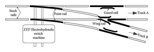
Rail transit has been widely used to resolve the problem of traffic jams because of its green, comfortable, and efficient advantages, and it has developed quickly [1, 2]. With the increasing number of rail transit lines and trains, the safe running of trains has also been under unprecedented pressure. The switch machine (SM) is an integral part of the railway signal system, and it is a critical equipment to realize the conversion of the running line of the rail vehicle [3, 4]. As shown in Figure 1, the SM can realize the switching between Track A and Track B, that is, the conversion of the line. However, the SM works in harsh environments such as rain, snow, and high temperatures for a long time, which aggravates the occurrence of its faults. Common faults include no-load faults, card gap faults, and multiple switching. Relevant research shows that [5] 40% of total signal unit faults of SM faults are incredibly high in fault frequency and risk. Therefore, it is of well-meaning to accurately grasp the state information of SM and carry out fault diagnosis (FD) research to ensure the safety of rail vehicles.

Details are in the caption following the image — **Figure 1**
Open in figure viewer PowerPoint

Schematic diagram of SM.

The core work of SM FD is extracting fault features from signals. The FD method based on vibration signal is a common method at present. Due to its nonlinear and nonstationary characteristics, it is difficult to accurately extract feature information. Therefore, it is necessary to use effective signal-processing methods to effectively extract feature information. For example, EMD, ICEEMDAN, VMD, and other[6–9] such methods usually show good performance in FD of rotating machinery, but the advantages in fault feature extraction of SM are not significant. With the continuous study of nonlinear dynamics, the nonlinear dynamics method based on entropy-based signal complexity measurement has received more attention. It is utilized to represent the feature in the vibration signals of switch machines and other mechanical equipment and extracts’ fault features [10]. The commonly used methods include permutation entropy (PE), sample entropy (SE), and fuzzy entropy (FE) [11–13]. However, the entropy of a single scale usually cannot fully reflect the irregularity of the signal, so the extracted features are not comprehensive. Based on this, multiscale PE (MPE), multiscale SE (MSE), and multiscale FE (MFE) have appeared one after another [14]. This kind of nonlinear dynamic method has achieved more results in fault detection. For instance, Lao et al. [15] applied MPE to signal measurement of the SM and combined it with the time-domain feature index to obtain a better feature extraction effect. Field experimental data verified the reliability of the MPE. Li et al. [16] used MSE to obtain the feature of the planetary reducer under nonstationary conditions for FD of the reducer. Zheng et al. [17] used MFE to reflect the intricacy of signals, and experiments verified the feasibility of MFE. Although this kind of nonlinear measurement method is multiscale, there are inherent defects in taking off the intricacy of vibration signals. For instance, the PE ignores the amplitude information, and the SE calculates the resource consumption. It is prone to mutation, and the membership function of the FE lacks physical meaning. In addition, the linear mean filtering will cause the above method to lose adequate signal feature information [18]. To conquer the shortcomings of the above models, Rostaghi [19, 20] developed a new nonlinear measurement model named dispersion entropy (DE). Compared to PE and SE, DE has strong antinoise ability, which considers the signal’s amplitude and has a faster calculation speed. In addition, DE is also combined with multiscale entropy to expand to multiscale DE (MDE). Wang et al. [21] used the synchrosqueezing window Fourier transform to decompose the transformer discharge signal and combine it with MDE to extract the characteristic information of the intrinsic mode components. The experiment’s consequences verify the ranking property of MDE under noise interference. Based on MDE, Hamed Azami et al. [22] developed the refined composite MDE (RCMDE). RCMDE has a more stable performance and can be applied to distinguish different types of dynamics. Zhao et al. [23] believed that FD ground on external magnetic flux leakage could identify various faults and proposed an engine FD method based on variational mode decomposition (VMD) and RCMDE. RCMDE is used to reconstruct the magnetic flux leakage signal, and experiments verify the superior performance of RCMDE. Liu et al. [24] proposed an optimized VMD and RCMDE model for chatter detection of thin-walled parts. RCMDE was used to detect milling chatter, and experiments determined the method’s feasibility. However, the average cumulative distribution function is used for mapping in RCMDE, and the nonlinear mapping ability needs to be improved. In addition, although RCMDE considers the absoluteness of the amplitude, it does not consider the relativity of the amplitude and cannot evaluate the fluctuation of the signal. In particular, the vibration signal of the SM has noticeable fluctuation when it fails, and the fault signal is a periodic signal, which is quite different from the signal of the rotating machinery. The above shortcomings restrict the feature extraction capability of RCMDE in the SM signal. Due to the shortcomings of RCMDE, this paper proposes a Gaussian distribution refined composite multiscale fluctuation DE (GGRCMFDE). Generalized Gaussian distribution (GGD) has attracted much attention in many noise modeling because of its flexible parameter form of the probability density function, and it is considered to be a substitute for cumulative normal distribution [25, 26]. In GGRCMFDE, the GGD is utilized to substitute the normal cumulative distribution function (NCDF) to improve the nonlinear mapping ability. Considering that RCMDE cannot analyze the fluctuation of signals, the fluctuation theory is introduced into GGRCMFDE [27] as a countermeasure to treating the fluctuation of time series.

When using GGRCMFDE to obtain the characteristics of time series signals, an intelligent FD method of an SM based on GGRCMFDE and an optimized support vector machine (SVM) is proposed. Considering that the performance of SVM is related to parameter setting [28], a fault identification method based on improving dung beetle optimization (IDBO)–optimized SVM is proposed. DBO is a new optimization algorithm proposed by Xue and Shen [29] in 2023, which has the strengths of solid optimization ability, fast convergence speed, and high solution precision. However, the algorithm still needs to focus on avoiding the local optimum [30]. Based on this, this paper introduces the Bernoulli chaotic map, golden section ratio strategy, and dynamic weight strategy [31–33] to improve the algorithm’s ability. An improved dung beetle algorithm is proposed, and standard test functions certify the practicability of IDBO. Finally, the proposed FD method of GGRCMFDE and IDBO–-SVM is utilized for the vibration signal data of the SM collected in the actual scene for analysis. The experiment conclusions show that the GGRCMFDE–IDBO–SVM has a more significant feature extraction quality. Compared to the comparison method, it can more clearly determine the fault type of the SM and has a more accurate fault recognition rate.

The rest of this paper is structured as follows. The theoretical knowledge of GGRCMFDE and IDBO–SVM is shown in Section 2. In Section 3, the superiority of IDBO is verified by using standard test functions. Section 4 determines the procedure of FD of the switch machine. In Section 5, the GGRCMFDE–IDBO–SVM is utilized for the switch machine’s experiment data and verification analysis. Section 6 draws conclusions based on the above research content.

2. Materials and Methods

2.1. GGRCMFDE

On the basis of RCMDE, GGRCMFDE is proposed by combining GGD theory and fluctuation entropy theory. The steps are as follows.

1.
For the time series x = {x_j, j = 1, 2, ⋅⋅⋅, N}, the GGD is utilized to map the time series to y, y = {y_j, j = 1, 2, ⋅⋅⋅, N}y_i ∈ (0, 1), that is,
(1)
where is the incomplete gamma function, Γ is the gamma function, is the given scale parameter, y is the possibility of random variables in GGD, and μ, σ are the mean and standard deviation (SD), respectively. β determines the shape of the distribution and β = 2 is the Gaussian distribution [26].
2.
By linear transformation, y is mapped to the scope of [1, 2, ⋯, e], that is,
(2)
where int is the rounding function and e is the number of categories.
3.
The embedding vector z_m,d,i is calculated according to the embedding dimension m and the delay d as
(3)
4.
By calculating the difference between adjacent elements of the embedding vector, the fluctuation vector F_m,d is obtained as
(4)
5.
By calculating all possible dispersion modes Ω corresponding to a fluctuation vector F_m,d, we get
(5)
where Ω is obtained by multiplying m-1 elements.
6.
Calculating the possibility of each dispersion mode as
(6)
where Num(Ω) is the number of wave vectors mapped to dispersion patterns.
7.
For the original data μ, the kth coarsening sequence is given by the following formula:
(7)
Then, the average possibility of the DE model is computed as
(8)
where is the probability of each possible distribution pattern at different starting points.
8.
For each scale τ, the GGRCMFDE entropy is defined as follows:
(9)

2.2. IDBO–SVM

2.2.1. DBO

The DBO is a new heuristic algorithm. The algorithm has superior performance. It mainly comes from the biological behavior process of dung beetles. The theory is as follows [29].

2.2.1.1. Rolling Ball Behavior

Dung beetles have a wonderful habit of making excrement into balls and then putting it to the ideal place. In the rolling process, the dung beetle needs to pass through the celestial clues. To maintain the dung ball rolling in a straight line:

(10)

where ς represents the current quantity of iterations; f_i(ς) is the place information of the i-th dung beetle at the ς-th iteration; k ∈ (0, 0.2] represents a permanent value, representing the betrayal coefficient; b is a permanent range of (0, 1); α is a ratio, taking −1 or 1; F^w represents the lowest place; and Δf is utilized to model the alter of light intensity.

2.2.1.2. Dancing Behavior

When the dung beetle meets a barrier and cannot go ahead, it must be repositioned by dancing to obtain a new path line. A tangent function is utilized to mimic the dance behavior to acquire a new orientation. Once the dung beetle triumphantly determines the other direction, it will keep on rolling the ball backward. So, the place update is established as follows:

(11)

where θ is the deflection angle pertaining to [0, π].

2.2.1.3. Reproductive Behavior

Dung balls are rolled to a safe place and hidden by dung beetles. Choosing the right spawning site is considerable for dung beetles to offer a great place for future generations. A boundary selection strategy is used to analog the spawning place of female dung beetles, which is defined as

(12)

where F^∗ is the present local best place, Pb^∗ and Qb^∗ represent the minimum and maximum borders of the spawning place, R = 1 − ς/ς_max, ς_max represent the maximum quantity of iterations, and Pb and Qb express the minimum and maximum borders of the optimization question, respectively.

Each female dung beetle only lays one egg in each iteration. In addition, the border scope of the spawning place is dynamically changed, which is mainly confirmed by R. Therefore, the place of the brooding ball is also dynamic during the iteration, which is defined as

(13)

where B_i(ς) is the place message of the i-th ball at the ς-th iteration. b₁ and b₂ are two unaided random vectors with a size of 1 × D and D is the dimension of the optimization question.

2.2.1.4. Foraging Behavior

It is required to build the best foraging place to direct small beetles foraging and simulate the foraging procedure of these dung beetles. Especially, the border of the best foraging region is defined as follows:

(14)

where Y^b represents the present local best place and Pb^b and Qb^b represent the minimum and maximum range of the best foraging place.

Thus, the location of the little dung beetle is updated as follows:

(15)

where M₁ denotes the random number that obeys the normal distribution and M₂ denotes the random vector pertaining to (0,1).

2.2.1.5. Stealing

Some dung beetles are considered thieves. In addition, F^b is the best food source. Therefore, it is presumed that the vicinity of F^b represents the best place to contest for food. The thief’s location information is renewed and can be defined as

(16)

where g is a random vector with a size of 1 × D, which obeys the positive distribution, and S is a constant.

2.2.2. IDBO–SVM

2.2.2.1. Bernoulli Chaotic Map

The traditional DBO algorithm generates random numbers to initialize the population position in the population initialization stage. The dung beetle in the population cannot traverse all the positions in the environment, resulting in poor optimization effects and low convergence speed. The Bernoulli map is a linear map with a uniform probability density distribution function and it has a good ergodicity. The iterative equation is as follows:

(17)

where A is a variable parameter, which usually takes 2.

2.2.2.2. Golden Section Ratio Strategy

The golden section ratio strategy is selected in the ball position update formula because the ball rolling process needs more accurate and stable control, and the algorithm needs a more globally effective search in the relatively early iteration stage. In addition, a more random and random search strategy is adopted when updating other locations, which can reasonably suit global exploration and local optimization and enhance the algorithm’s performance. The golden section ratio formula can be expressed as

(18)

where r₁ and r₂ represent the random numbers in the interval (0,1). It is utilized to calculate the new candidate solution of dung beetle. f₁ and f₂ are the current position information of the other two dung beetles in the algorithm, which is used to calculate the new candidate solution. Its selection can promote the exchange of information between individuals and accelerate the search process.

Therefore, the improved position update formula of the rolling ball dung beetle can be expressed as

(19)

(20)

2.2.2.3. Dynamic Weight Strategy

The position update formula of the stealing dung beetle will renew its place based on the current individual optimal value, which quickly falls into the local optimum. More attention is paid to local optimization and convergence in the subsequent iteration stage. At the same time, the dynamic weight strategy can adaptively adjust the global search intensity according to the current stage and adaptively adjust the total search and local development. The weight k₁ is more prominent in the early stage of iteration so that the dung beetle can explore a better area near the optimal dung beetle. The weight k₂ increases gradually in the later stage of the iteration so that the dung beetle can leap out of the local optimum. The two parameters can be expressed as

(21)

The enhanced place update formula is expressed as

(22)

The steps for using the IDBO to optimize the SVM are as follows:

1.
Initialization of dung beetles: randomly initialize the place of dung beetles (kernel function parameters and penalty factors) and IDBO algorithm parameters.
2.
The fitness value is computed: the place of each dung beetle is brought into the SVM for training and testing, and the classification precision of the train set is utilized as the fitness value of the dung beetle.
3.
Updating the location of dung beetles: the IDBO is utilized to renew the location of each dung beetle.
4.
Judge whether the boundary is crossed: check whether the updated dung beetle position is within the predetermined range and reinitialize if it exceeds the range.
5.
Update the optimal solution: compare the fitness values of all dung beetles and update the optimal dung beetle’s place and the optimal fitness value.
6.
Iteration and determine the end condition: duplicate Steps 2–5 until the maximum iteration algebra is achieved and the optimal dung beetle position and optimal fitness value are output.

3. SM FD Framework

GGRCMFDE is applied to acquire the fault feature of the vibration data of the SM. On this basis, a FD method for the SM is proposed in combination with IDBO–SVM. The steps are as follows:

1.
Assuming that the SM has N fault states, the quantity of samples for each state is consistent, and GGRCMFDE extracts the fault feature information of each state.
2.
The feature vector is constructed, and 70% of the data is randomly choosen as the training dataset to train IDBO–SVM, and the residual 30% of the samples are used as test samples to test IDBO–SVM.
3.
The training dataset is input into the IDBO–SVM for training, and the trained classifier is tested by using the test samples.
4.
The classifier’s output results realize the switch machine’s fault location.

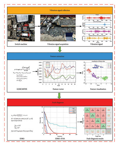
The proposed FD framework of the SM based on GGRCMFDE and IDBO–SVM is shown in Figure 2.

4. Simulation Analysis

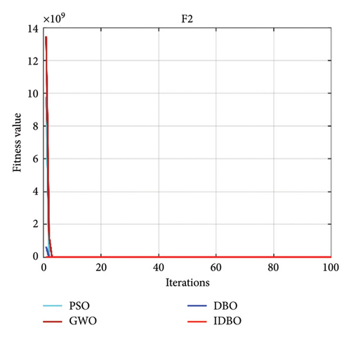
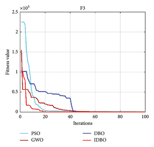
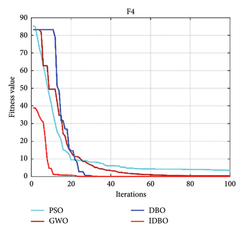
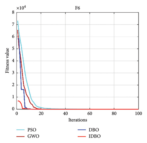
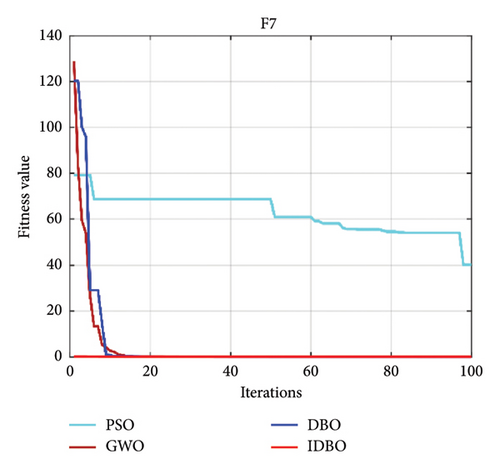
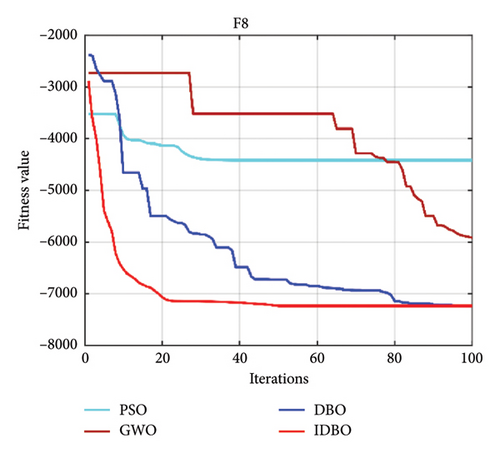
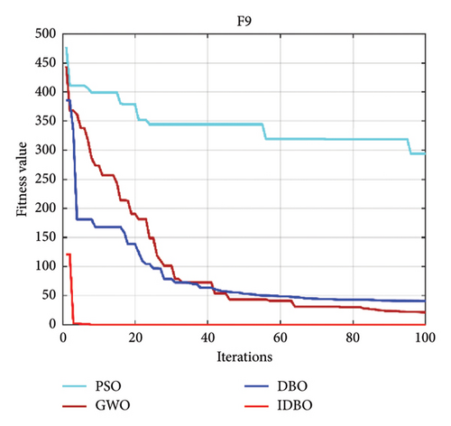
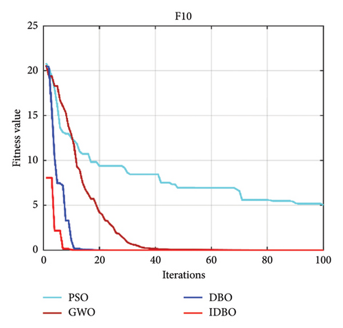
Intelligent optimization algorithms and their improved algorithms generally verify the algorithm’s performance through standard test functions. Here, we choose a standard test function used in the literature [34] to certify the feasibility of the IDBO. The standard test function is as follows (Table 1), where F1–F7 is an unimodal test function, and F8–F10 is applied to test the search quality of the IDBO. The quantity of iterations of the IDBO is set to 100, and the quantity of populations is 30. The property of the IDBO is realized by comparing it with other algorithms. Here, the particle swarm optimization (PSO) algorithm is selected as the representative of the classical method, the gray wolf optimization (GWO) algorithm is selected as the representative of the widely used algorithm, and the original DBO is selected as the representative of the latest algorithm. The property of the above algorithms is compared with that of IDBO. To prove the reliability of the test results, each optimization algorithm runs 10 times, respectively, and the optimal and average results of 10 experimental consequences are recorded. The test results of each algorithm among the 10 test functions [34] are shown in Figures 3(a), 3(b), 3(c), 3(d), 3(e), 3(f), 3(g), 3(h), 3(i), 3(j), and 3(k). Table 2 shows the results of 10 experimental records. In Figures 3(a), 3(b), 3(c), 3(d), 3(e), 3(f), 3(g), 3(h), 3(i), 3(j), and 3(k), we can see that no matter which test function is used, IDBO shows significant performance. The optimization speed is obviously better than other algorithms, and it also has good advantages in optimization accuracy, but it cannot be intuitively displayed. Through Table 2, we can see that IDBO has an irreplaceable advantage in optimization accuracy. Both the best results and the average results can confirm this conclusion.

Table 1. Standard test functions.

Function	V_no	Range
	30	[−100, 100]
	30	[−10, 10]
	30	[−100, 100]
F₄(x) = max_i{\|x_i\|, 1 ≤ i ≤ n}	30	[−100, 100]
	30	[−30, 30]
	30	[−100, 100]
	30	[−128, 128]
	30	[−500, 500]
	30	[−5.12, 5.12]
	30	[−32, 32]

Table 2. Comparison of algorithm’s results (10 times).

F	IDBO		DBO		PSO		GWO
F	Best	Ave	Best	Ave	Best	Ave	Best	Ave
F1	1.19E−44	5.46E−13	4.43E−35	5.39E−23	22.5915	26.99244	0.00024	0.000782
F2	3.08E−31	3.66E−24	1.38E−21	1.35E−10	18.4835	24.32147	0.0028	0.00505
F3	5.58E−42	1.41E−05	1.47E−23	0.00253	710.3255	901.1903	23.2278	147.0941
F4	4.21E−24	1.08E−12	1.61E−16	2.65E−05	2.7366	3.6006	0.2515	0.63096
F5	27.28553	27.88629	27.0564	27.47177	6079.394	12,832.56	28.1418	28.77026
F6	0.008305	0.934896	0.160268	0.489528	16.23034	24.47	1.316885	2.228565
F7	0.000113	0.000456	0.002201	0.009895	42.69871	69.75816	0.005073	0.009729
F8	−12548.1	−11297	−9233.517	−7827.664	−4050.88	−3581.26	−6965.37	−5884.2
F9	0	0	0	0.886518	224.3948	271.1002	12.6272	22.34901
F10	8.8E−16	8.8E−16	7.9E−15	1.24E−10	4.593725	5.221556	0.004038	0.006215

Note: Bold values represent the smallest values.

It needs to be more comprehensive to verify the performance of IDBO only by the optimal and average results. Here, we use the statistical test method to verify further. The Friedman test [35] is often utilized to test the quality of intelligent optimization algorithms. The statistical test results can effectively prove the rationality of the method. Table 3 shows the consequences of the Friedman test. The rank sum and average rank of IDBO are the best. Therefore, the performance of IDBO is also the most superior, followed by DBO, and the worst is PSO. Here, we combine Figure 3 to draw this conclusion accurately. Based on the above analysis, we are very confident that the performance of IDBO is superior, and it has unquestionable advantages in optimization accuracy and speed. It shows that introducing the Bernoulli chaotic map, golden section ratio strategy, and dynamic weight strategy to improve DBO is reasonable and practical.

Table 3. Friedman’s rank test.

Methods	Rank sum	Average rank	Rank
IDBO	16	1.6	1
DBO	18	1.8	2
PSO	38	3.8	4
GWO	28	2.8	3

5. Experimental Verification

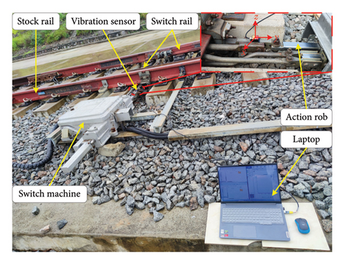
The ZYJ7 electrohydraulic SM is used in a vehicle section of the Nanning subway. Its structure mainly includes a power, conversion, and representation locking mechanism. To verify the reliability of the GGRCMFDE in the FD of the SM, we collected the vibration signal of the actual operation scene for verification. In Figure 4, we can see the SM and its data collection equipment. The switch is completed by the action bar, and the action bar can significantly sense the state of the SM. Therefore, we arrange the vibration sensor (HWT605) on the action bar of the SM. The HWT605 sensor transmits three orthogonal vibration acceleration signals to the laptop in real time through serial communication (RS-232). The normal switching action time of the switch is about 8 s, and the sampling frequency is set to 200 Hz. Four states of the SM are collected: normal, no-load fault, card gap fault, and vibration signal of multiple switches. Each state is continuously collected 50 times.

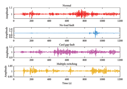
In Figure 5, we can see the acquired vibration data of the SM under different fault scenarios. There is a particular difference between the SM’s vibration data and the rotating machinery’s vibration signal, such as bearings and gears. The vibration data of the rotating machinery present the characteristics of periodic impact. In the three stages of the SM start-up process, switch rail implementation, and SM locking, there are generally three peaks, and the signal shows the characteristics of fluctuation, which is consistent with the operation status of the switch machine. There are some differences in the vibration data of each fault scene, indicating that the vibration signals of the SM contain rich feature information, and the reliable feature extraction method can realize the effective identification of the SM fault.

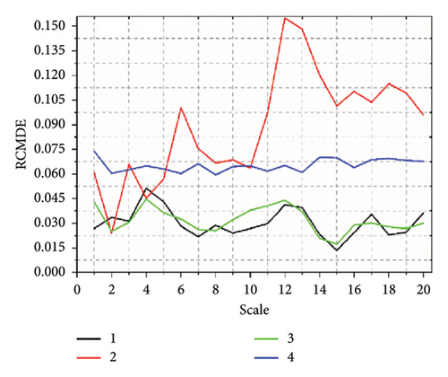
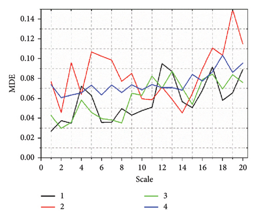
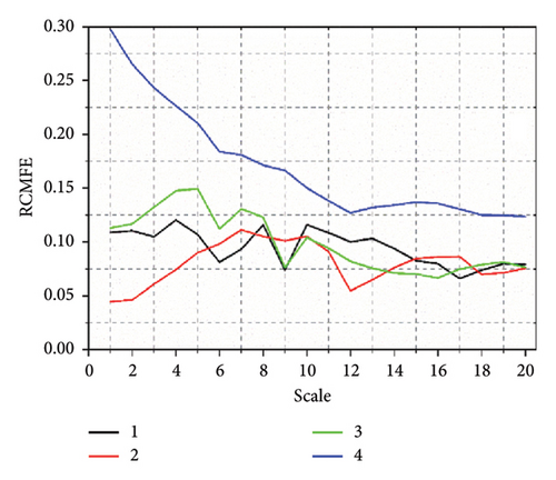
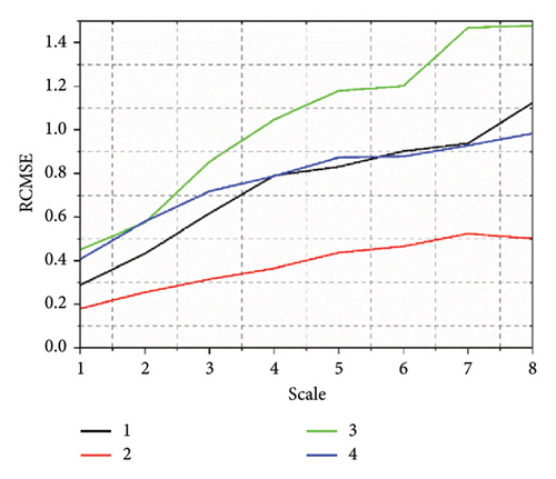
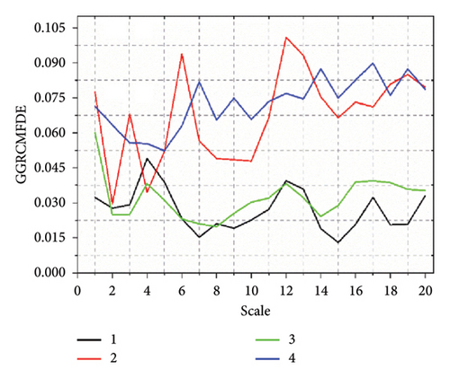
After collecting the vibration signal of the SM fault scene, the GGRCMFDE extracts the feature information. GGRCMFDE has six parameters: data length N, shape parameter β, embedding dimension m, class number e, time delay d, and maximum scale factor S. In fact, d = 1 is recommended because d > 1 may be aliasing [19]. According to the authors in [19], e = 6 is used for all signals, although the range 2 < e < 9 leads to similar results. For the choice of S, we choose S = 20 to ensure the number of entropy values. In most entropy-based nonlinear dynamics methods, the m range is generally 2–6 [36, 37], where we take the intermediate value. The length of the SM signal is related to the sampling frequency, where N is set to the actual sampling signal length. After setting the parameter values of GGRCMFDE, GGRCMFDE is utilized to obtain the characteristics of the four state scenarios of the switch machine. Each state scenario obtains a 50 × 20 eigenvalue. The difference in the collected data will lead to a change in the entropy value. Even the data in the same state scenario will also be different. To judge the effect of GGRCMFDE feature extraction, we calculated the SD of the entropy value in each state scenario. The lesser the SD is, the better the effect of feature extraction will be. Figure 6 is the SD of GGRCMFDE feature extraction under four fault scenarios, where 1, 2, 3, and 4 represent the normal state of the switch machine, no-load fault, card gap fault, and multiple switching faults, respectively. Here, the methods commonly used in the paper in recent years are choosen as contrast models to determine the properties of GGRCMFDE, including RCMDE [38], MDE [39], refined composite multiscale FE (RCMFE) [37], and refined composite multiscale SE (RCMSE) [40]. In Figure 6(e) the SD of each state entropy value is relatively small. The SD at most scales is less than 0.1, indicating that the effect of GGRCMFDE feature extraction is relatively stable. It also proved that GGRCMFDE performs superior in the SM signal feature extraction model. Compared to GGRCMFDE, the performance of the other comparison methods is significantly insufficient. RCMDE fluctuates wildly at State 2, with more data and with a SD greater than 0.1. Although the SD of MDE in state two is better than that of RCMDE, the SD of other states shows an upward trend, and the overall feature extraction ability is weaker than that of RCMDE, which is also consistent with the feature extraction ability of RCMDE in practical application due to MDE [38]. The SD of each state entropy value of RCMFE is more significant than that of GGRCMFDE, and more data are more significant than 0.1. The scale factor of RCMSE is set to 8, andso in the experiment, we find that the feature extraction ability of RCMSE for nonperiodic signals is weak. When the scale factor is too significant, effective information cannot be extracted. The corresponding feature is 0, and the scale factor is 8. Therefore, we set the scale factor of RCMSE to 8. However, the SD of each state entropy value is more extensive, indicating that the extracted features are significantly different, and the shortcomings of RCMSE in the feature extraction of SM signals are also judged. Based on the above comparative analysis, GGRCMFDE has irreplaceable advantages over RCMDE, MDE, RCMFE, and RCMSE in the feature extraction method of the SM signal.

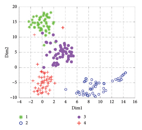
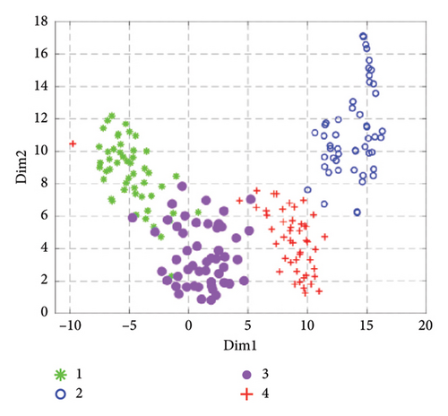
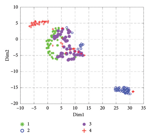
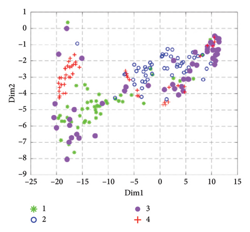
Although the SD can reflect the ability of GGRCMFDE feature extraction, it needs to be more comprehensive. t-Distributed stochastic neighbor embedding (t-SNE) is often utilized to characterize the effect of feature extraction [41–43]. Therefore, from the visualization perspective, we use t-SNE to map the extracted features to a two-dimensional space and obtain a visual image of the features as shown in Figure 7. In Figure 7(e), the features of the four states can be effectively separated and better aggregated together, indicating that feature extraction is effective and can provide a reasonable basis for accurate classification. In the comparison method, the features extracted by RCMDE in State 3 and State 4 are more dispersed, and the distinction between State 1 and state 3 needs to be more pronounced, which is easy to cause classification errors. The features extracted by MDE are scattered, and more samples of State 1 and State 3 are mixed together, showing that its feature extraction ability is weaker than that of RCMDE and GGRCMFDE. The features extracted by RCMFE are only effectively separated in the samples of State 2 and State 4, and the feature overlap degree of State 1 and State 3 is higher, so the probability of fault classification error is higher. The visualization effect of RCMSE is the worst. Although some samples can be aggregated together, more features are mixed together, indicating that its feature extraction ability in the SM signal is insufficient, which is in compliance with the consequence of the previous section analysis. On the basis of the above visual analysis of feature extraction methods, the significant ability of GGRCMFDE in the feature extraction of SM signals can be clearly proved.

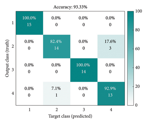
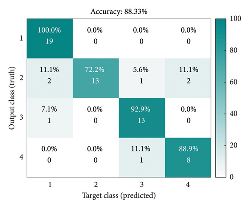
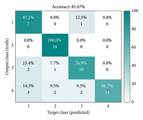
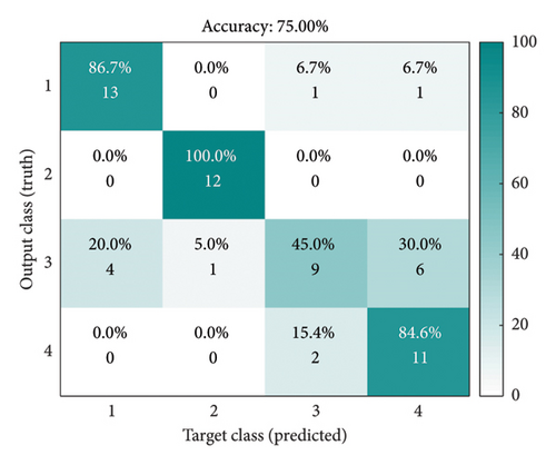
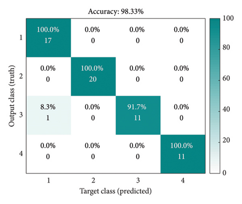
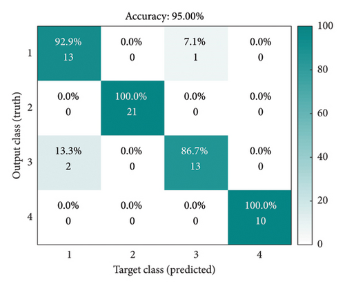
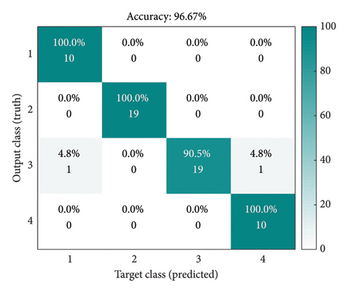
The above analysis only analyzes the method’s performance intuitively but cannot give a quantitative evaluation index. Therefore, we use IDBO–SVM as a classification method to classify the extracted features and accurately judge the method’s feasibility through the final FD accuracy. In the IDBO–SVM, the quantity of populations is set to 30 [44], and the quantity of iterations is 100, and this is mainly determined by the performance of IDBO in the F1–F10 test functions. The total sample of the FD of the SM is 200. Here, all the samples are disrupted; hence, 70% of the samples are chosen as training samples and the residual 30% are used as test samples to avoid the impact of inaccurate classification results due to sample contingency. At the same time, five experiments were carried out, and the average value of the five experiments was selected as the final diagnosis result. The confusion matrix obtained is shown in Figure 8, where we choose a confusion matrix similar to the average value of FD. The FD results obtained by combining GGRCMFDE with IDBO–SVM are 98.33%, and the diagnosis results obtained by (a), (b), (c), and (d) and the other four methods are 93.66%, 89.51%, 82.66%, and 74.21%, respectively. Compared to these four comparison methods, the precision of GGRCMFDE–IDBO–SVM is advanced by 4.67%, 8.82%, 15.67%, and 24.21%, respectively, and the precision is remarkably raised, which once again shows the reliable feature extraction capability of GGRCMFDE. In order to verify the feasibility of the proposed IDBO–SVM, the diagnostic effect of PSO–RF proposed in the literature [45] as a classifier is compared. The feature extraction method is still GGRCMFDE, and the average FD result is 96%, as shown in Figure 8(f). Compared to PSO–RF, the proposed method has a higher diagnostic accuracy of 2.33%. In addition, the FD method of the SM proposed in the literature [15] is selected as a comparison method to verify the superiority of GGRCMFDE–IDBO–SVM. The average FD result obtained in the literature [15] is 95.41%, as shown in Figure 8(g). The accuracy of GGRCMFDE–IDBO–SVM is 2.92% higher than that of the method proposed in the literature [15]. The superiority of GGRCMFDE in the FD of switch machines is powerfully demonstrated through the combination of quantitative analysis and intuitive qualitative analysis above. The GGRCMFDE–IDBO–SVM can offer academic support for the FD of SM.

6. Conclusions

The vibration signal of the SM shows the characteristics of nonperiodic fluctuation, and the signal contains less feature information. The traditional feature extraction method has been unable to fulfill the needs of the FD of the switch machine. Based on this, a new nonlinear dynamic model is developed to increase the signal feature extraction capacity of the switch machine. An FD method based on GGRCMFDE and IDBO–SVM is proposed. GGRCMFDE–IDBO–SVM is suitable for FD of SM and can provide good theoretical support for intelligent maintenance of switch machines. The conclusions are as follows:

1.
The GGD and fluctuation theory are introduced to develop GGRCMFDE, which has better feature extraction capability than the other four comparison methods and has strong applicability in the signal feature extraction of switch machines.
2.
The Bernoulli chaotic map, the golden section ratio, and the dynamic weight strategy are used to improve the DBO. The proposed IDBO has good optimization ability and can resolve the question of SVM parameter setting.
3.
The FD method of the SM based on GGRCMFDE and IDBO–SVM is proposed. The diagnostic accuracy of the GGRCMFDE–IDBO–SVM is 98.33%. It is more evident than comparison methods.

Although GGRCMFDE has good adaptability and superior feature extraction ability in the feature extraction of SM signals, its parameter setting problem is ground on experience. In the next step, GGRCMFDE parameter setting research will be carried out to improve the performance of GGRCMFDE further.

Conflicts of Interest

The authors declare no conflicts of interest.

Funding

The research was supported by the National Natural Science Foundation of China (Grant no. U22A2053), the Guangxi Natural Science Foundation (Grant no. 2024JJB160040), the Major Science and Technology Project of Guangxi Province of China (Grant no. Guike AB23062076), the Guangxi Manufacturing Systems and Advanced Manufacturing Technology Key Laboratory Director Fund (Grant no. 24-050-44-S015), the Innovation Project of Guangxi Graduate Education (Grant no. YCBZ2024013), the Major Talent Project in Guangxi Zhuang Autonomous Region and the Guangxi Key Laboratory of Precision Navigation Technology and Application (Grant no. DHKL2418), and the Guilin University of Electronic Technology.

Open Research

Data Availability Statement

Data are available on request from the authors.

References

1 Wu J., He D., Li J. et al., Temporal Multi-Resolution Hypergraph Attention Network for Remaining Useful Life Prediction of Rolling Bearings, Reliability Engineering & System Safety. (2024) 247, https://doi.org/10.1016/j.ress.2024.110143.
10.1016/j.ress.2024.110143
Web of Science® Google Scholar
2 He D., Zhao J., Jin Z., Huang C., Zhang F., and Wu J., Prediction of Bearing Remaining Useful Life Based on a Two-Stage Updated Digital Twin, Advanced Engineering Informatics. (2025) 65, https://doi.org/10.1016/j.aei.2025.103123.
10.1016/j.aei.2025.103123
Web of Science® Google Scholar
3 Cao Y., Ji Y., Sun Y., and Su S., The Fault Diagnosis of a Switch Machine Based on Deep Random Forest Fusion, IEEE Intelligent Transportation Systems Magazine. (2023) 15, no. 1, 437–452, https://doi.org/10.1109/mits.2022.3174238.
10.1109/MITS.2022.3174238
Web of Science® Google Scholar
4 Wen W., Liu Y., Bai Y., and Meng Q., A Feature Pseudo-Fusion Method for Intelligent Fault Diagnosis of Electro-Hydraulic Switch Machine Inspired by Contrastive Learning, Part F: Journal of Rail and Rapid Transit. (2023) .
10.1177/09544097231165093
Google Scholar
5 Sun Y., Cao Y., and Li P., Contactless Fault Diagnosis for Railway Point Machines Based on Multi-Scale Fractional Wavelet Packet Energy Entropy and Synchronous Optimization Strategy, IEEE Transactions on Vehicular Technology. (2022) 71, no. 6, 5906–5914, https://doi.org/10.1109/tvt.2022.3158436.
10.1109/TVT.2022.3158436
Web of Science® Google Scholar
6 Zou X., He D., Jin Z., Wei Z., and Miao J., Intelligent Diagnosis Method of Bearing Fault Based on ICEEMDAN and Ghost-IRCNN, Proceedings of the Institution of Mechanical Engineers-Part C: Journal of Mechanical Engineering Science. (2023) 237, no. 13, 3115–3130, https://doi.org/10.1177/09544062221144390.
10.1177/09544062221144390
Web of Science® Google Scholar
7 Feng K., Ni Q., Chen Y., Ge J., and Liu Z., A Cyclostationarity-Based Wear Monitoring Framework of Spur Gears in Intelligent Manufacturing Systems, Structural Health Monitoring. (2023) .
10.1177/14759217221147018
Web of Science® Google Scholar
8 He D., Wu J., Jin Z., Huang C., Wei Z., and Cai Y., AGFCN: A Bearing Fault Diagnosis Method for High-Speed Train Bogie Under Complex Working Conditions, Reliability Engineering & System Safety. (2025) 258.
10.1016/j.ress.2025.110907
Web of Science® Google Scholar
9 Jin Z., Chen D., He D., Sun Y., and Yin X., Bearing Fault Diagnosis Based on VMD and Improved CNN, Journal of Failure Analysis and Prevention. (2023) 23, no. 1, 165–175, https://doi.org/10.1007/s11668-022-01567-7.
10.1007/s11668-022-01567-7
Web of Science® Google Scholar
10 Tian J., Yi G. W., Fei C. W., Zhou J., Ai Y. T., and Zhang F. L., Quantum Entropy-Based Hierarchical Strategy for Inter-Shaft Bearing Fault Detection, Structural Control and Health Monitoring. (2021) 28, no. 12, https://doi.org/10.1002/stc.2839.
10.1002/stc.2839
PubMed Web of Science® Google Scholar
11 Tan H., Xie S., Zhou H., Ma W., Yang C., and Zhang J., Sensible Multiscale Symbol Dynamic Entropy for Fault Diagnosis of Bearing, International Journal of Mechanical Sciences. (2023) 256, https://doi.org/10.1016/j.ijmecsci.2023.108509.
10.1016/j.ijmecsci.2023.108509
Web of Science® Google Scholar
12 Delgado-Bonal A. and Marshak A., Approximate Entropy and Sample Entropy: A Comprehensive Tutorial, Entropy. (2019) 21, no. 6, https://doi.org/10.3390/e21060541, 2-s2.0-85068069891.
10.3390/e21060541
PubMed Web of Science® Google Scholar
13 Jin Z. and Sun Y., Bearing Fault Diagnosis Based on VMD Fuzzy Entropy and Improved Deep Belief Networks, Journal of Vibration Engineering & Technologies. (2023) 11, no. 2, 577–587, https://doi.org/10.1007/s42417-022-00595-9.
10.1007/s42417-022-00595-9
Web of Science® Google Scholar
14 Wang Z., Li G., Yao L., Qi X., and Zhang J., Data-Driven Fault Diagnosis for Wind Turbines Using Modified Multiscale Fluctuation Dispersion Entropy and Cosine Pairwise-Constrained Supervised Manifold Mapping, Knowledge-Based Systems. (2021) 228, https://doi.org/10.1016/j.knosys.2021.107276.
10.1016/j.knosys.2021.107276
PubMed Web of Science® Google Scholar
15 Lao Z., He D., Wei Z. et al., Intelligent Fault Diagnosis for Rail Transit Switch Machine Based on Adaptive Feature Selection and Improved LightGBM, Engineering Failure Analysis. (2023) 148, https://doi.org/10.1016/j.engfailanal.2023.107219.
10.1016/j.engfailanal.2023.107219
Web of Science® Google Scholar
16 Li Y., Feng K., Liang X., and Zuo M. J., A Fault Diagnosis Method for Planetary Gearboxes Under Non-Stationary Working Conditions Using Improved Vold-Kalman Filter and Multi-Scale Sample Entropy, Journal of Sound and Vibration. (2019) 439, 271–286, https://doi.org/10.1016/j.jsv.2018.09.054, 2-s2.0-85054556011.
10.1016/j.jsv.2018.09.054
Web of Science® Google Scholar
17 Zheng J., Cheng J., Yang Y., and Luo S., A Rolling Bearing Fault Diagnosis Method Based on Multi-Scale Fuzzy Entropy and Variable Predictive Model-Based Class Discrimination, Mechanism and Machine Theory. (2014) 78, 187–200, https://doi.org/10.1016/j.mechmachtheory.2014.03.014, 2-s2.0-84899435486.
10.1016/j.mechmachtheory.2014.03.014
Web of Science® Google Scholar
18 Zheng J., Pan H., Liu Q., and Ding K., Refined Time-Shift Multiscale Normalised Dispersion Entropy and Its Application to Fault Diagnosis of Rolling Bearing, Physica A: Statistical Mechanics and Its Applications. (2020) 545, https://doi.org/10.1016/j.physa.2019.123641.
10.1016/j.physa.2019.123641
Web of Science® Google Scholar
19 Rostaghi M., Azami H., ostaghi M., and Azami H., Dispersion Entropy: A Measure for Time-Series Analysis, IEEE Signal Processing Letters. (2016) 23, no. 5, 610–614, https://doi.org/10.1109/lsp.2016.2542881, 2-s2.0-84964343754.
10.1109/LSP.2016.2542881
Web of Science® Google Scholar
20 Yan X. and Jia M., Intelligent Fault Diagnosis of Rotating Machinery Using Improved Multiscale Dispersion Entropy and mRMR Feature Selection, Knowledge-Based Systems. (2019) 163, 450–471, https://doi.org/10.1016/j.knosys.2018.09.004, 2-s2.0-85053671718.
10.1016/j.knosys.2018.09.004
Web of Science® Google Scholar
21 Wenbo W., Lin S., Bin W., and Min Y., Partial Discharge Feature Extraction Based on Synchrosqueezed Windowed Fourier Transform and Multi-Scale Dispersion Entropy, Measurement and Control. (2020) 53, no. 7-8, 1078–1087, https://doi.org/10.1177/0020294020932346.
10.1177/0020294020932346
Google Scholar
22 Azami H., Rostaghi M., Abásolo D., and Escudero J., Refined Composite Multiscale Dispersion Entropy and Its Application to Biomedical Signals, IEEE Transactions on Biomedical Engineering. (2017) 64, no. 12, 2872–2879, https://doi.org/10.1109/TBME.2017.2679136, 2-s2.0-85029350745.
10.1109/TBME.2017.2679136
PubMed Web of Science® Google Scholar
23 Zhao S., Chen Y., Rehman A. U. et al., Detection of Interturn Short-Circuit Faults in DFIGs Based on External Leakage Flux Sensing and the VMD-RCMDE Analytical Method, IEEE Transactions on Instrumentation and Measurement. (2022) 71, 1–12, https://doi.org/10.1109/tim.2022.3186061.
10.1109/tim.2022.3186061
Web of Science® Google Scholar
24 Liu X., Wang H., Li M., Wang Z., and Meng B., Milling Chatter Detection of Thin-Walled Parts Based on GA-SE-SCK-VMD and RCMDE, The International Journal of Advanced Manufacturing Technology. (2023) 124, no. 3-4, 945–958, https://doi.org/10.1007/s00170-022-10235-x.
10.1007/s00170-022-10235-x
Web of Science® Google Scholar
25 Dytso A., Bustin R., Poor H. V., and Shamai S., Analytical Properties of Generalized Gaussian Distributions, Journal of Statistical Distributions and Applications. (2018) 5, no. 1, 6–40, https://doi.org/10.1186/s40488-018-0088-5, 2-s2.0-85062698524.
10.1186/s40488-018-0088-5
Google Scholar
26 Dhandapani R., Mitiche I., McMeekin S., and Morison G., A Novel Bearing Faults Detection Method Using Generalized Gaussian Distribution Refined Composite Multiscale Dispersion Entropy, IEEE Transactions on Instrumentation and Measurement. (2022) 71, 1–12, https://doi.org/10.1109/tim.2022.3187717.
10.1109/TIM.2022.3187717
Web of Science® Google Scholar
27 Azami H. and Escudero J., Amplitude-and Fluctuation-Based Dispersion Entropy, Entropy. (2018) 20, no. 3, https://doi.org/10.3390/e20030210, 2-s2.0-85044248886.
10.3390/e20030210
Web of Science® Google Scholar
28 Agrawal A. K. and Chakraborty G., Semi-Supervised Implementation of SVM-Based Error-Correcting Output Code for Damage-Type Identification in Structures, Structural Control and Health Monitoring. (2022) 29, no. 8, https://doi.org/10.1002/stc.2967.
10.1002/stc.2967
PubMed Web of Science® Google Scholar
29 Xue J. and Shen B., Dung Beetle Optimizer: A New Meta-Heuristic Algorithm for Global Optimization, The Journal of Supercomputing. (2023) 79, no. 7, 7305–7336, https://doi.org/10.1007/s11227-022-04959-6.
10.1007/s11227-022-04959-6
Web of Science® Google Scholar
30 Zhang R. and Zhu Y., Predicting the Mechanical Properties of Heat-Treated Woods Using Optimization-Algorithm-Based BPNN, Forests. (2023) 14, no. 5, https://doi.org/10.3390/f14050935.
10.3390/f14050935
Web of Science® Google Scholar
31 Alexan W., Elkandoz M., Mashaly M., Azab E., and Aboshousha A., Color Image Encryption Through Chaos and Kaa Map, IEEE Access. (2023) 11, 11541–11554, https://doi.org/10.1109/access.2023.3242311.
10.1109/ACCESS.2023.3242311
Web of Science® Google Scholar
32 Li Z., A Local Opposition-Learning Golden-Sine Grey Wolf Optimization Algorithm for Feature Selection in Data Classification, Applied Soft Computing. (2023) 142, https://doi.org/10.1016/j.asoc.2023.110319.
10.1016/j.asoc.2023.110319
PubMed Web of Science® Google Scholar
33 Jin Z., He D., and Wei Z., Intelligent Fault Diagnosis of Train Axle Box Bearing Based on Parameter Optimization VMD and Improved DBN, Engineering Applications of Artificial Intelligence. (2022) 110, https://doi.org/10.1016/j.engappai.2022.104713.
10.1016/j.engappai.2022.104713
Web of Science® Google Scholar
34 Jin Z., He D., Lao Z., Wei Z., Yin X., and Yang W., Early Intelligent Fault Diagnosis of Rotating Machinery Based on IWOA-VMD and DMKELM, Nonlinear Dynamics. (2023) 111, no. 6, 5287–5306, https://doi.org/10.1007/s11071-022-08109-8.
10.1007/s11071-022-08109-8
Web of Science® Google Scholar
35 Li X., Zhang S., Yang L., and Shao P., Neighborhood-Search-Based Enhanced Multi-Strategy Collaborative Artificial Bee Colony Algorithm for Constrained Engineering Optimization, Soft Computing. (2023) 27, no. 19, 13991–14017, https://doi.org/10.1007/s00500-023-08491-4.
10.1007/s00500-023-08491-4
Web of Science® Google Scholar
36 Jin Z., Xiao Y., He D., Wei Z., Sun Y., and Yang W., Fault Diagnosis of Bearing Based on Refined Piecewise Composite Multivariate Multiscale Fuzzy Entropy, Digital Signal Processing. (2023) 133, https://doi.org/10.1016/j.dsp.2022.103884.
10.1016/j.dsp.2022.103884
Web of Science® Google Scholar
37 Li J., Zheng J., Pan H., Tong J., Feng K., and Ni Q., Two-Dimensional Composite Multi-Scale Time-Frequency Reverse Dispersion Entropy-Based Fault Diagnosis for Rolling Bearing, Nonlinear Dynamics. (2023) 111, no. 8, 7525–7546, https://doi.org/10.1007/s11071-023-08250-y.
10.1007/s11071-023-08250-y
Web of Science® Google Scholar
38 Lu Y., Zhu D., Zhao D., Zhu D., Sun D., and Gao Q., A Novel Bearing Fault Diagnosis Algorithm Based on Adaptive Weighted Multi-View Learning, IEEE Transactions on Instrumentation and Measurement. (2023) 72, 1–13, https://doi.org/10.1109/tim.2023.3291000.
10.1109/TIM.2023.3329222
PubMed Google Scholar
39 Zhou N. and Wang L., Triple Feature Extraction Method Based on Multi-Scale Dispersion Entropy and Multi-Scale Permutation Entropy in Sound-Based Fault Diagnosis, Frontiers in Physics. (2023) 11, https://doi.org/10.3389/fphy.2023.1180595.
10.3389/fphy.2023.1180595
Web of Science® Google Scholar
40 Zhang J., Zhu X., Li W. et al., Refined Composite Multiscale Fuzzy Entropy Based Fault Diagnosis of Diesel Engine, Journal of Low Frequency Noise, Vibration and Active Control. (2023) 42, no. 1, 420–437, https://doi.org/10.1177/14613484221129754.
10.1177/14613484221129754
Web of Science® Google Scholar
41 Lao Z., He D., Jin Z., Liu C., Shang H., and He Y., Few-Shot Fault Diagnosis of Turnout Switch Machine Based on Semi-supervised Weighted Prototypical Network, Knowledge-Based Systems. (2023) 274, https://doi.org/10.1016/j.knosys.2023.110634.
10.1016/j.knosys.2023.110634
PubMed Web of Science® Google Scholar
42 He D., Lao Z., Jin Z., He C., Shan S., and Miao J., Train Bearing Fault Diagnosis Based on Multi-Sensor Data Fusion and Dual-Scale Residual Network, Nonlinear Dynamics. (2023) 111, no. 16, 14901–14924, https://doi.org/10.1007/s11071-023-08638-w.
10.1007/s11071-023-08638-w
Web of Science® Google Scholar
43 He D., Zhang Z., Jin Z., Zhang F., Yi C., and Liao S., RTSMFFDE-HKRR: A Fault Diagnosis Method for Train Bearing in Noise Environment, Measurement. (2025) 239, https://doi.org/10.1016/j.measurement.2024.115417.
10.1016/j.measurement.2024.115417
Web of Science® Google Scholar
44 He D., Xu Y., Jin Z., Liu Q., Zhao M., and Chen Y., A Zero-Shot Model for Diagnosing Unknown Composite Faults in Train Bearings Based on Label Feature Vector Generated Fault Features, Applied Acoustics. (2025) 232, https://doi.org/10.1016/j.apacoust.2025.110563.
10.1016/j.apacoust.2025.110563
Web of Science® Google Scholar
45 Jin Z., He D., Ma R., Zou X., Chen Y., and Shan S., Fault Diagnosis of Train Rotating Parts Based on Multi-Objective VMD Optimization and Ensemble Learning, Digital Signal Processing. (2022) 121, https://doi.org/10.1016/j.dsp.2021.103312.
10.1016/j.dsp.2021.103312
Web of Science® Google Scholar

All articles

Generalized Gaussian Distribution Refined Composite Multiscale Fluctuation Dispersion Entropy and Its Application in Fault Diagnosis of Switch Machine

Abstract

1. Introduction