Imaging-Based Instance Segmentation of Pavement Cracks Using an Improved YOLOv8 Network
Abstract
An improved YOLOv8 model, YOLOv8-NETC, is proposed in this study for fine-grained crack recognition through instance segmentation. YOLOv8-NETC is designed and enhanced with four self-developed modules. First, ablation studies were conducted to assess the effectiveness of each module. The model’s accuracy and speed were evaluated based on parameters such as mean average precision (mAP50) and model weight (MW). The experimental results show significant improvements in accuracy, storage efficiency, and processing speed. Compared to the original network, YOLOv8-NETC achieved a 6.5% increase in mAP50, a 6.1% average reduction in MW and parameters, and an 8.5% improvement in FPS. Subsequently, YOLOv8-NETC was compared with other state-of-the-art models across three datasets, including the crack type dataset, crack trueness dataset, and the public Crack500 dataset. The experimental results demonstrate that the proposed model achieved the best recognition performance on all datasets. Furthermore, YOLOv8-NETC showed superior robustness against interference and computational efficiency compared to other benchmark models.
1. Introduction
Crack detection and severity assessment are essential for evaluating the safety of structures. Advances in computer vision technology have significantly improved the effectiveness of automated crack detection methods, enhancing both accuracy and efficiency over manual approaches [1].
There are two primary approaches to image-based crack detection: rule-based methods and machine learning-based methods [2]. Rule-based methods involve manually defining scenarios and crack characteristics, followed by the application of image processing techniques and filters to identify cracks. While these methods do not require training, their effectiveness is limited by the predefined rules [3, 4]. Due to the diversity of crack morphology and the complexity of environmental disturbances in real-world scenarios, these methods usually lack robustness and are difficult to cope with the detection needs under different conditions.
In contrast, machine learning methods are widely used for their ability to learn and adapt to complex, evolving situations. Although traditional machine learning methods enhance flexibility through manual feature extraction, the feature design process often requires extensive human intervention and involves high computational complexity. For instance, while support vector machine (SVM)-based methods reduce the need for large training datasets, their performance is limited when handling large-scale datasets or more complex crack patterns [5]. Similarly, the minimum rectangle covering approach and random forest frameworks demonstrate certain advantages in specific scenarios but lack sufficient generalization capabilities [6–8]. Furthermore, many methods struggle to distinguish cracks from pseudo-cracks, such as surface textures or shadows, particularly in high-noise environments [9–11].
Deep learning, a subset of machine learning, offers even greater potential for crack detection by automatically extracting features and providing stronger generalization [12]. Convolutional neural networks (CNNs), which excel at image processing, have been particularly effective in crack detection. For instance, Dorafshan [13] found that CNNs outperformed traditional edge detectors in both accuracy and computational efficiency. Two-stage detection methods, such as region CNNs (R-CNNs), combine CNNs with additional processing steps to improve detection accuracy [14]. Recent studies have applied these methods to tasks such as concrete bridge crack detection [15] and the monitoring of surface cracks in structures [16]. Variants like Fast R-CNN, Faster R-CNN, and Mask R-CNN have been developed to further enhance detection speed and accuracy [17–20]. Although two-stage detection methods, such as Mask R-CNN, achieve high accuracy by using region proposal networks and pixel-level segmentation, they are often limited by slower processing speeds. In real-time detection scenarios, this becomes a significant drawback, as both high accuracy and fast inference are critical for effective performance. In contrast, single-stage detection methods, such as the Single Shot Multibox Detector (SSD) and You Only Look Once (YOLO), offer simpler and more efficient end-to-end pipelines, enabling real-time detection. While SSD is known for its speed, YOLO is preferred for crack detection due to its superior accuracy, especially for small and complex objects like cracks [21, 22]. YOLO’s end-to-end training and global reasoning allow it to better capture the spatial features of cracks, improving detection performance. Studies have shown that YOLOv3, YOLOv4, and their variants can achieve high accuracy in detecting and classifying cracks across various settings [23–25]. In contrast, SSD, despite its speed, often struggles with precision and tends to produce more false positives, which is undesirable in crack detection. Overall, YOLO offers a better balance of accuracy and efficiency, making it the more suitable choice for crack detection. While single-stage detection methods have improved detection efficiency, there is still room for enhancement in detecting small cracks and recognizing cracks in complex backgrounds.
In segmentation tasks, semantic segmentation provides pixel-level classification but fails to identify and distinguish individual crack instances. To address this, instance segmentation, which combines object detection and semantic segmentation, has been applied to crack detection. This approach assigns a unique identifier to each crack instance, as demonstrated by the development of poly YOLO and Mirror-YOLO [26, 27]. While current instance segmentation methods can differentiate individual cracks, their accuracy and computational efficiency are still limited, particularly when dealing with multiple crack types and complex backgrounds. The YOLO series has demonstrated strong performance in crack detection [28–30], with YOLOv8 offering improved generalization and detection speed over previous versions [31–33]. However, despite advances in detection speed, the YOLO series still faces challenges in extracting detailed crack features, which impacts its ability to detect a wide variety of cracks effectively.
Previous studies have shown several limitations. Most of them focused on crack detection in simple environments, such as plain concrete surfaces or pavements, without fully considering how to adapt to different scenes or distinguish cracks in complex backgrounds. This makes solving more realistic and practical problems challenging. Additionally, although YOLOv8 improved detection speed compared to its predecessors, its accuracy in detecting tiny cracks remains low, mainly due to insufficient feature extraction capabilities. Balancing detection accuracy and efficiency is crucial for practical applications, which highlights the need for further development in crack detection technology.
To address the aforementioned challenges, this study first integrates four distinct computer vision techniques and proposes an enhanced YOLOv8-based pixel-level instance segmentation network. The proposed network comprises the following key components: (1) the NKBlock module (N); (2) the EnhanceC2f module (E); (3) a novel loss function (T); and (4) an innovative connection method (C). As a result of these improvements, the resulting network is named YOLOv8-NETC. In order to validate the model’s performance in detecting cracks within complex backgrounds, two custom datasets were created: the crack type dataset and the crack trueness dataset. Subsequently, ablation studies were conducted on the crack type dataset, optimizing for accuracy, storage efficiency, and inference speed to identify the most effective architecture for the YOLOv8 encoder. Finally, comparative experiments involving multiple models were carried out across three datasets, including one widely used public benchmark dataset, to thoroughly assess the performance of the proposed method.
The rest of the paper is organized as follows. Section 2 introduces the YOLOv8 and YOLOv8-NETC architectures. Section 3 presents the dataset, comparison models, and implementation details. Section 4 presents the evaluation metrics, ablation study results, and comparative experimental results. Section 5 summarizes the findings of this study and the advantages of the improved model while providing directions for future work.
2. Improved Detection Model
2.1. Overview
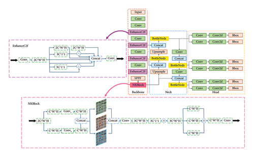
Ultralytics YOLOv8 builds on the YOLOv5 structure and draws on the strengths of other YOLO versions for further use in engineering practice. The framework is shown in Figure 1.
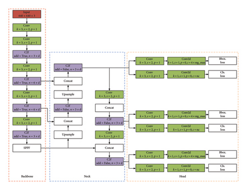
CSPDarkNet53, a network designed for target detection, is the YOLOv8 backbone network. Compared to YOLOv5, YOLOv8 uses the C2f module instead of the C3 module in the network. This network has more jump-layer connections. In addition, there are additional splits in the network for better data management. The YOLOv8 neck adopts the idea of a path aggregation network (PAN). Feature maps of different scales are fused by PAN, which enhances the ability of the network to understand image objects and avoids the loss of too much spatial information in deep layers of the network. Compared with YOLOv5, the most significant change in YOLOv8 is in the head. YOLOv8 adopts a decoupled head structure, separating the detection head from the classification, and the final branch outputs the boundary and category. Through decoupling, a universal basic network can be trained. Then, different heads can be connected according to different tasks.
In the following, we first show the architecture of each module in the improved approach. This is followed by clarifying the motivation for the design of each module and the advantages of the improvements.
2.2. NKBlock
Convolutional operations play a pivotal role in deep neural networks by effectively extracting local feature information from input tensors. In the NKBlock (see Figure 2), we employ two distinct convolutional operations (Conva and Convb), applied to different parts of the input tensor. Compared to the convolution operations (Conv and Conv2d) in Section 2.1, Grouped Convolution aims at extracting features at different scales and encourages the module to learn richer feature representations.

Grouped Convolution is a technique that divides the input tensor’s channels into groups and applies convolution operations separately to each group. This approach reduces the number of parameters in each convolutional kernel, thereby lowering computational complexity while retaining the expressive power of the convolutional layer. In the NKBlock, after grouping the input tensor, we apply convolution operations to each group individually. This method not only preserves the independence of features but also enhances the network’s feature extraction capability.
The function relationship for Grouped Convolution is similar to that of standard convolution, but with a grouping operation applied along the channel dimension of the input tensor. Suppose the input tensor is , where H and W represent the height and width of the input tensor, and Cin is the number of input channels. Grouped Convolution divides the input channels Cin into G groups, with each group containing channels. Convolution operations are then applied separately to each group.
Max pooling operations are a commonly used down sampling technique, preserving spatial information by retaining local maxima and reducing the dimensionality of feature maps. In the NKB module, we apply max pooling operations before convolutional operations to maintain feature information while reducing computational complexity. This strategy allows us to effectively capture multiscale information from the input tensor, enhancing the module’s perceptual and expressive capabilities.
2.3. EnhanceC2f
In this section, we provide a detailed theoretical analysis of the design principles and operational mechanisms of the EnhanceC2f module (see Figure 3). Two convolution operations are performed in the module, and their respective roles need to be clearly explained in the description. Therefore, we have distinguished between the two convolutions, naming them Conv1 and Conv2.

2.4. Global Information
2.5. Two-Factor Loss Function
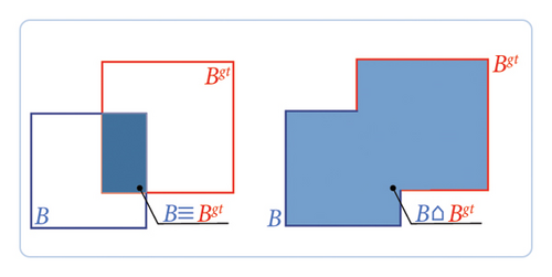
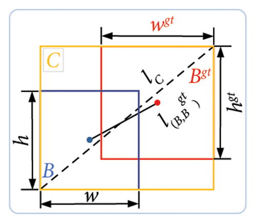
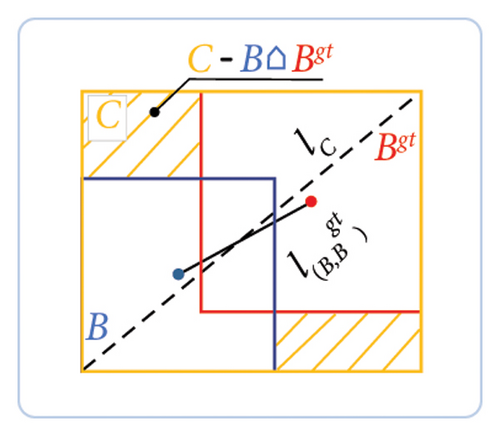
MIoU, as an improved loss function, effectively overcomes the limitations of traditional IoU in handling the geometric and positional relationships between predicted boxes and ground truth boxes. By incorporating bounding box information and distance metrics, MIoU offers a more comprehensive evaluation of target box matching, particularly excelling in road crack detection. It not only accurately identifies fine cracks but also effectively distinguishes cracks from background noise (such as water stains, branches, and expansion joints), enhancing the accuracy and robustness of detection. Overall, MIoU significantly improves the detection performance of complex road cracks by considering geometric information and distance relationships.
2.6. End-to-End Connection
To improve the performance of the case segmentation model, a new feature fusion method is proposed. Specifically, we deal with the problem of efficiently integrating multiscale feature maps. We introduce a concatenation-based fusion approach where feature graphs from different scales are concatenated before being fed to the detection head. We present a mathematical formula to express this fusion method and emphasize its advantages in improving the accuracy of target detection (as shown in equations (13), (14)).
3. Experimental Program
Experiments were conducted on three datasets with different crack types and different noise backgrounds to validate the improved method. In addition, six well-known deep learning networks, YOLOv8, YOLOv5, SOLOv2, Mask R-CNN, CondInst, and SparseInst, were used for the comparative study. The implementation details and selection of hyperparameters for the training process are presented.
3.1. Datasets
Generally, pavement cracks are categorized into three types, namely, longitudinal cracks, transverse cracks and fatigue cracks, which have a nonnegligible impact on pavement structure. Previous studies have focused more on performing automatic crack detection and segmentation rather than recognizing different crack types. To achieve pixel-level pavement crack segmentation, three crack datasets, namely, the public Crack500 dataset and two of our customized datasets, the crack type dataset and the crack trueness dataset, were introduced.
3.1.1. Crack Type Dataset
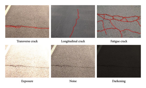
The crack type dataset is our customized dataset. In road pavement crack detection, crack direction is essential for structural health evaluation. Longitudinal cracks are often related to the load-bearing capacity of the pavement, while transverse cracks are typically influenced by environmental factors such as temperature fluctuations and moisture changes. Fatigue cracks, which result from repeated traffic loads over time, are also significant in assessing the durability and longevity of pavement structures. By distinguishing these crack types in our dataset, the proposed method can classify crack directions, which enhances its ability to address more complex analysis tasks in pavement management and maintenance. A total of 1371 images with a resolution of 512 × 512 were generated from 457 photos. Objective conditions, such as the structural surface complexity and weather variability, pose significant challenges for crack recognition. As a result, the images in the dataset vary in terms of crack type, brightness, contrast, and noise. In this study, the training and validation sets were randomly divided into 70% and 30%, respectively. Specifically, there were 960 images for training and 411 images for validation. The number of crack types in the dataset is shown in Table 1. The cracks in each image were manually marked with locations and assigned labels for training and validation. Some image samples are shown in Figure 6.
| Crack type | Training set | Validation set | Total number |
|---|---|---|---|
| Longitudinal | 346 | 148 | 494 |
| Transverse | 310 | 133 | 443 |
| Fatigue | 304 | 130 | 434 |
| Total number | 960 | 411 | 1371 |
3.1.2. Crack500 Dataset
In the Crack500 dataset, 500 photos of 2000 × 1500 pixels of Temple University’s main campus were obtained by Yang et al. [34]. The pavement material for this dataset is asphalt, while the photos contain different contrasts and shadows. The Crack500 dataset is a collection of images specifically designed for crack detection and segmentation tasks, widely used for training and evaluating image segmentation models. The dataset is tailored for crack detection, containing a large number of images depicting various types and forms of cracks. To accommodate the memory limitations of the computational system, each image is divided into 16 subimages. As a result of this preprocessing step, the total number of available images increases to 3368. In this study, the dataset is split into a training set and a validation set. The training set consists of 1896 images, while the validation set contains 1472 images. The crack source images and annotated images are shown in Figure 7.

3.1.3. Crack Trueness Dataset
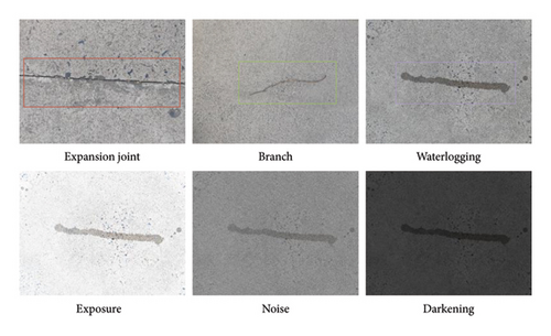
In crack identification, branches, expansion joints, and water stains introduce additional interference. To improve the model’s ability to identify environmental interferences, this study proposes a new crack image dataset called “crack trueness.” This dataset not only includes various interference factors but also contains different types of cracks from the crack type dataset. The crack samples are randomly selected, with the number of samples for each interference type matching the number of samples for each crack type.
As Figure 8 shows, a total of 300 RGB images with a size of 576 × 768 pixels were collected, including images of expansion joints, water stains, and branches. To augment the data volume and diversity, image transformation methods were applied with the following settings: exposure adjustment (brightness scaling factor ranging from 0.8 to 1.2), contrast adjustment (contrast scaling factor ranging from 0.8 to 1.2), and noise addition (Gaussian noise with a mean of 0 and a standard deviation ranging from 0 to 10 pixel intensity units). After enhancement using Photoshop, the dataset contains a total of 1200 interference images and 1200 crack images. Similar to the crack type dataset, this study randomly divided the training set and validation set at a 70%:30% ratio. The quantities of different interferences in the dataset are shown in Table 2. Detection and segmentation annotation files were prepared using LabelImg and LabelMe software, respectively, to mark the interferences.
| Type of interference | Training set | Validation set | Total number |
|---|---|---|---|
| Expansion joint | 280 | 120 | 400 |
| Waterlogging | 280 | 120 | 400 |
| Branch | 280 | 120 | 400 |
| Longitudinal cracks | 280 | 120 | 400 |
| Transverse cracks | 280 | 120 | 400 |
| Fatigue cracks | 280 | 120 | 400 |
| Total number | 1680 | 720 | 2400 |
3.2. Comparison Models
- •
YOLOv8: Please refer to Section 2.1 of this study.
- •
YOLOv5 is a version developed by Ultralytics. YOLOv5 uses mosaic data augmentation on the input side, which allows multiple images to be combined at a certain scale. The CSP structure is referenced in the backbone and neck, which improves the feature fusion capability of the model.
- •
SOLOv2: decouples mask generation into a mask kernel branch and a mask feature branch. This decoupling allows dynamic segmentation of each instance in the image, while a new matrix NMS is utilized to improve redundant detection frame removal efficiency.
- •
Cascade Mask R-CNN: A cascade structure is used that contains a detection head and a segmentation head in each stage. The output of each stage is used as the input for the next stage. The cascade structure of each stage can gradually process samples of increasing difficulty, which helps to improve detection and segmentation accuracy.
- •
CondInst: This approach solves the instance segmentation problem using a fully convolutional network and does not require resizing the feature maps, which leads to more accurate boundaries for high-resolution masks. The CondInst can dynamically generate the corresponding mask head depending on the instance, which makes the mask head compact and leads to faster inference.
- •
SparseInst: A sparse instance activation map (IAM) is used to highlight foreground targets. The IAM obtains instance features by highlighting instance pixels and aggregating the features, avoiding incorrect localization problems in the center or region approach. In addition, IAM predicts objects one-to-one and avoids nongreat value suppression.
3.3. Implementation Details
All the experiments performed in this study were based on Facebook’s PyTorch library. Deep learning machines configured with the CentOS 7 operating system and Linux workstations were used for model training. Two NVIDIA Ampere A100 graphics processing units (GPUs) with 80 GB of memory were adopted to perform the tasks quickly and efficiently.
In this study, the model was optimized by backpropagation using stochastic gradient descent (SGD) with momentum. In this approach, each parameter update depended on both the current gradient and the effect of the momentum in the previous steps. The application of the momentum method accelerated the convergence rate, and the parameter values were relatively stable. Standard Gaussian initialization was used to initialize the neural network weights. The algorithm had an initial learning rate of α = 0.001, a momentum parameter of β = 0.937, and a weight decay of γ = 0.0005. In addition, a batch size of 1 and a base size of 16 were used for the anchors.
4. Experimental Results and Discussion
4.1. Evaluation Metrics
Instance segmentation provides pixel-level information on the location, shape and number of cracked regions. Two categories were set up in this study: cracks and background. Crack and background pixels were defined as positive and negative categories, respectively. Depending on the actual and predicted results, pixel sums were categorized as true positives (TPs), true negatives (TNs), false positives (FPs) and false negatives (FNs). Based on the prediction results, four commonly used evaluation metrics, precision (PRE), mean accuracy (mAP), recall (REC) and balanced F1 score (F1), were used to assess the performance of the model. They were calculated using equations (15), (16), (17), (18), respectively. The PRE refers to the percentage of accurately predicted crack pixels out of all the results predicted as cracks. The mAP represents the performance of the model on different categories. The REC refers to the percentage of accurately predicted crack pixels out of the sum of all actual crack pixels. The F1 score combines both PRE and REC.
4.2. Ablation Study
The following four components made up the bulk of the work in this study: the NKBlock (N), the EnhanceC2f (E), the two-factor loss function (T), and the end-to-end connection (C). Ablation experiments were performed to confirm the contribution of each component to crack instance segmentation. Notably, the main difference between the improved and traditional architectures is in the module section. Therefore, the original YOLOv8 model was used as the baseline approach in Tables 3 and 4 to compare the accuracy and speed of ablation experiments, respectively. Our custom Crack Type Dataset was used for the ablation experiments. The arrows in both Table 3 and Table 4 represent the change magnitude relative to the baseline. In Table 3, the change magnitude is calculated by taking the difference, while in Table 4, it is calculated through normalization, which involves dividing the difference by the baseline data.
| The utilized network | YOLOv8 | NKBlock | EnhanceC2f | Two-factor loss function | End-to-end connectivity | Instance segmentation | |||
|---|---|---|---|---|---|---|---|---|---|
| Precision (%) | mAP50 (%) | Recall (%) | F1 (%) | ||||||
| Baseline | ✓ | 78.2 | 72.7 | 73.5 | 75.8 | ||||
| YOLOv8-N | ✓ | ✓ | 78.1↓0.1 | 72.5↓0.2 | 73.2↓0.3 | 75.6↓0.2 | |||
| YOLOv8-NC | ✓ | ✓ | ✓ | 76.7↓1.5 | 73.9↑1.2 | 74.7↑1.2 | 75.7↓0.1 | ||
| YOLOv8-NTC | ✓ | ✓ | ✓ | ✓ | 79.4↑1.2 | 75↑2.3 | 74.2↑0.7 | 76.7↑0.9 | |
| YOLOv8-E | ✓ | ✓ | 78.5↑0.3 | 76.3↑3.6 | 77.3↑3.8 | 77.9↑2.1 | |||
| YOLOv8-EC | ✓ | ✓ | ✓ | 81.3↑3.1 | 76.9↑4.2 | 75.6↑2.1 | 78.3↑2.6 | ||
| YOLOv8-ETC | ✓ | ✓ | ✓ | ✓ | 77.2↓1 | 77.5↑4.8 | 78.7↑5.2 | 77.9↑2.2 | |
| YOLOv8-T | ✓ | ✓ | 82.7↑4.5 | 77.2↑4.5 | 75.2↑1.7 | 78.8↑3 | |||
| YOLOv8-C | ✓ | ✓ | 76.2↓2 | 76.5↑3.8 | 79.2↑5.7 | 77.7↑1.9 | |||
| YOLOv8-NETC | ✓ | ✓ | ✓ | ✓ | ✓ | 78.9↑0.7 | 77.4↑4.7 | 77.7↑4.2 | 78.3↑2.5 |
- Note: The arrows represent the change magnitude relative to the baseline, which is calculated by the difference.
| The utilized network | Instance segmentation | |||
|---|---|---|---|---|
| Model weight (MB) | Parameters | Average change | FPS | |
| Baseline | 6.8 | 3,258,259 | 0 | 515 |
| YOLOv8-N | 5.8↓14.7% | 2,758,361↓15.3% | −15% | 345↓33% |
| YOLOv8-NC | 5.8↓14.7% | 2,758,361↓15.3% | −15% | 556↑8% |
| YOLOv8-NTC | 6.2↓8.8% | 2,983,833↓8.4% | −8.6% | 400↓22.3% |
| YOLOv8-E | 6.5↓4.4% | 3,109,099↓4.6% | −4.5% | 208↓59.6% |
| YOLOv8-EC | 6.5↓4.4% | 3,109,099↓4.6% | −4.5% | 455↓11.7% |
| YOLOv8-ETC | 6.9↑1.5% | 3,334,571↑2.3% | 1.9% | 270↓47.6% |
| YOLOv8-T | 6.8 | 3,266,713↑0.3% | 0.1% | 526↑2.1% |
| YOLOv8-C | 6.8 | 3,258,649↑0.01% | 0 | 435↓15.5% |
| YOLOv8-NETC | 6.4↓5.9% | 3,051,691↓6.3% | −6.1% | 559↑8.5% |
- Note: The arrows represent the change magnitude relative to the baseline, which is calculated through normalization by dividing the difference by the baseline data.
4.2.1. Precision Evaluation
As shown in Table 3, YOLOv8 with the T module provided the largest improvement across all the metrics in terms of the F1 and PRE parameters. With respect to the baseline, YOLOv8-T increased F1 by 3 points (pts) and PRE by 4.5. YOLOv8, with the C module, provided the largest improvement across the metrics in terms of the REC parameter. At the baseline, YOLOv8-C had an increase in REC of 5.7 pts. YOLOv8, and the E, T, and C modules together, provided the largest improvement across the metrics in the mAP50 parameter. With respect to the baseline, YOLOv8-ETC increased the mAP50 by 4.8 pts. Among all the models in Table 3 for which accuracy was compared, the models for which all parameters improved were YOLOv8-E, YOLOv8-EC, YOLOv8-T, and YOLOv8-NETC. Moreover, the N module alone had a negative effect on the model’s accuracy. With respect to the baseline, YOLOv8-N had a mAP50 of 0.2 pts, an F1 of 0.2 pts, a PRE of 0.1 pts, and a REC of 0.3 pts. However, when N was integrated with other modules, the effectiveness of the approach was enhanced. Figure 9 better illustrates the specific effects of each module.
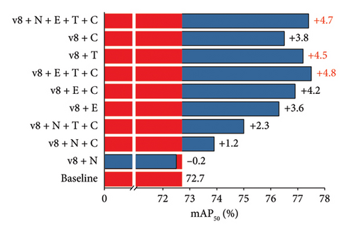
As Figure 9 shows, at the baseline, YOLOv8-E, YOLOv8-T, and YOLOv8-C increased the mAP50 by 3.6 pts, 4.5 pts, and 3.8 pts, respectively. Therefore, the E, T, and C modules all contributed to the increase in the model’s accuracy. After combining the three modules, YOLOv8-EC and YOLOv8-ETC increased the mAP50 by 4.2 pts and 4.8 pts, respectively, compared with the baseline. To address the accuracy degradation of YOLOv8-N (with the baseline mAP50 decreased by 0.2 pts), the T module and C module were added based on YOLOv8-N. With the baseline mAP50, YOLOv8-NC and YOLOv8-NTC increased mAP50 by 1.2 pts and 2.3 pts, respectively. After the combination of all the modules, YOLOv8-NETC increased the mAP50 by 4.7 pts.
4.2.2. Speed and Storage Efficiency Evaluation
Table 4 summarizes the MW and P of networks with different modules. Smaller MW and P indicate reduced storage requirements for the model. In this study, we compared all networks with the original network and calculated the average percentage change in MW and P. A greater reduction in MW and P (i.e., a smaller average change) reflects higher storage efficiency relative to the original network. Furthermore, FPS values for different modules are provided to directly assess the model’s inference speed. Typically, a higher FPS indicates a faster response time in real-world applications.
In the analysis of the average change in MW and P, different models exhibited varying degrees of optimization compared to the baseline model. YOLOv8-N and YOLOv8-NC both showed an average change of −15%, demonstrating significant improvements in storage and computational efficiency. YOLOv8-NTC showed an average change of −8.6%, indicating effective optimization in both storage and computation. YOLOv8-NETC exhibited an average change of −6.1%, also indicating higher resource utilization efficiency. In contrast, YOLOv8-E and YOLOv8-EC showed smaller average changes of −4.5%, while YOLOv8-ETC showed a slight performance improvement of +1.9%. YOLOv8-T and YOLOv8-C exhibited minimal changes, with average changes of 0.1% and 0%, respectively, suggesting that their storage and computational efficiency were nearly identical to the baseline model.
In the evaluation of real-time inference performance, FPS was used as a key metric to reflect model inference speed. YOLOv8-NETC stood out with a FPS of 559, an 8.5% increase over the baseline FPS of 515, demonstrating significant improvement in real-time responsiveness. YOLOv8-NC also performed well, with a FPS of 556, a 8% improvement over the baseline, providing superior real-time performance while maintaining an appropriate model size. However, YOLOv8-N and YOLOv8-NTC showed reduced FPS, with 345 FPS and 400 FPS, respectively, representing a 33% and 22.3% decrease compared to the baseline. This indicates that although optimizations in storage and computation were applied, real-time inference performance was significantly affected. YOLOv8-E and YOLOv8-ETC further demonstrated reductions in FPS, with values of 208 FPS and 270 FPS, respectively, suggesting that while storage optimization was achieved, inference speed significantly declined. In contrast, YOLOv8-T showed a slight FPS increase to 526 FPS, reflecting a 2.1% improvement, while YOLOv8-C had a FPS of 435 FPS, representing a 15.5% decrease compared to the baseline.
In conclusion, YOLOv8-NETC performs exceptionally in both storage efficiency and real-time inference, with a notable advantage in real-time inference speed. While YOLOv8-N and YOLOv8-NC showed significant optimization in storage and computation, their FPS performance lagged behind that of YOLOv8-NETC. YOLOv8-NTC and YOLOv8-T exhibited a more balanced optimization, particularly in terms of storage and computation. With its efficient inference speed and storage optimization, YOLOv8-NETC holds substantial potential for real-time applications, especially in scenarios where high real-time performance is critical, as its efficient inference capability can meet performance demands.
4.2.3. Comprehensive Evaluation: Balancing Accuracy, Speed, and Storage Efficiency
In practical applications, achieving a balance between speed, accuracy, and storage efficiency is crucial for effective detection tasks. This study simultaneously considers accuracy (Section 4.2.1), speed, and efficiency (Section 4.2.2) to provide a comprehensive evaluation. Figure 10 highlights the trade-offs between speed, accuracy, and efficiency for the evaluated models, offering a more integrated understanding of their performance.
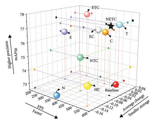
According to Figure 10, although YOLOv8-ETC achieves the highest accuracy among all models, its inference speed and storage efficiency are both inferior to Baseline. Specifically, YOLOv8-ETC is slower and consumes more memory. In contrast, YOLOv8-N and YOLOv8-NC demonstrate smaller memory footprints, but show only minimal improvements in accuracy. Among the tested models, YOLOv8-NETC exhibits the most balanced performance, with significant improvements in accuracy, speed, and storage efficiency. Specifically, YOLOv8-NETC not only achieves the fastest speed but also attains the second-highest accuracy (with mAP50 only 0.1% points lower than YOLOv8-ETC). While YOLOv8-NETC has a moderate storage efficiency, models with smaller memory footprints compromise significantly on accuracy and speed, whereas those with higher accuracy are noticeably slower. Therefore, YOLOv8-NETC stands out by providing good accuracy while maintaining high speed and low memory usage, making it more advantageous for practical applications. Given its balanced performance, YOLOv8-NETC was selected for further comparison with other advanced networks in this study.
4.2.4. Loss Curves and Visualization
Figure 11 illustrates the training results of the improved YOLO models. The number of training epochs was set to 180. Typically, the training loss measures how well the model fits the training data. The validation loss was used to assess the model’s generalization ability. During training, the training and validation losses of each model initially decreased sharply and gradually stabilized at approximately 1 as the number of epochs increased. The final training and validation loss values of YOLOv8 were 1.6 and 1.198, respectively. After adding the four modules, the training and validation loss values of YOLOv8-NETC were reduced to 1.563 and 1.185, respectively. The final training and validation losses of all the other models were greater than those of YOLOv8-NETC. Overall, the model with all four improvements added (YOLOv8-NETC) had a smoother loss curve decline and the best testing performance.
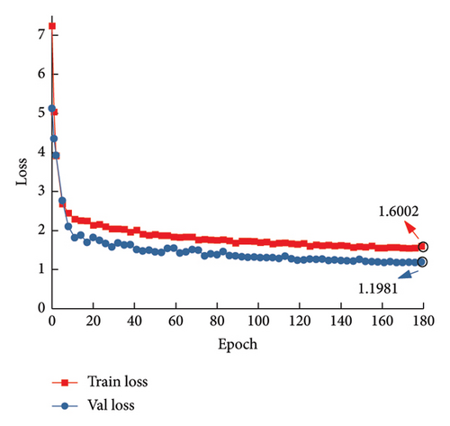
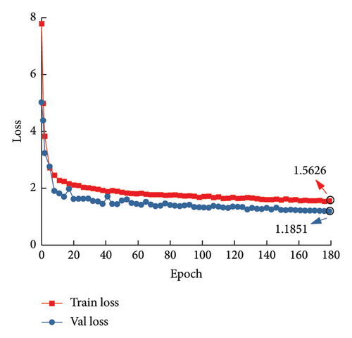
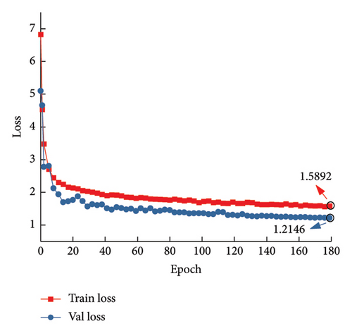

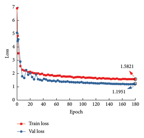
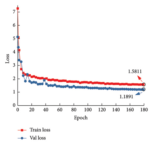
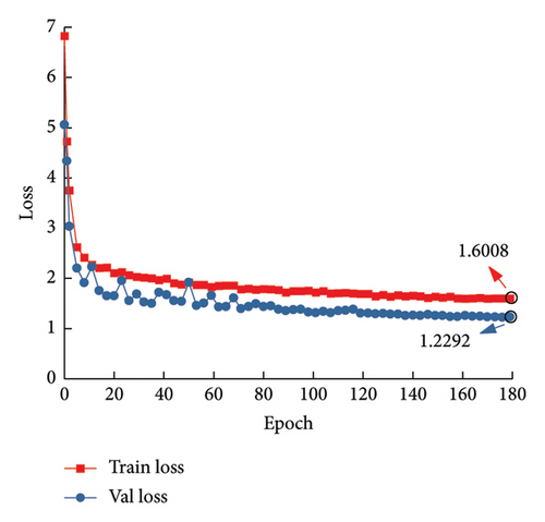
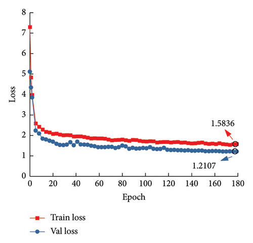
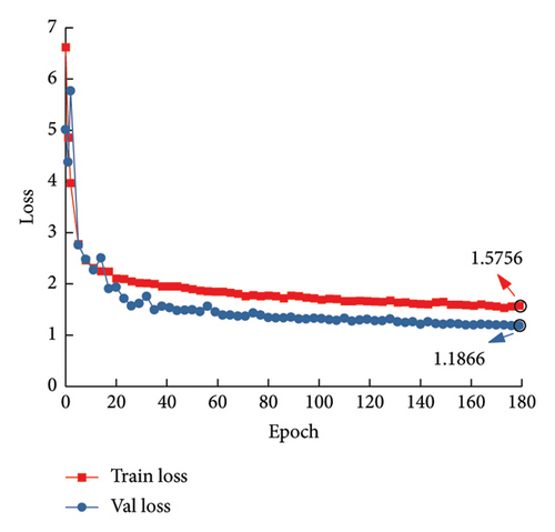
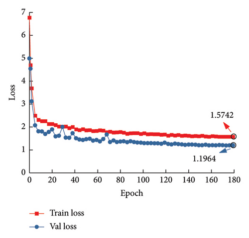
Figure 12 compares the ground-truth annotations with the prediction results, with precision metrics mapped onto the detection outcomes. For image (a) and (b), the models YOLO-NTC, -EC, and -ETC misidentified an expansion joint as a longitudinal crack. This mistake was not observed in the other models, indicating that certain configurations may be more prone to this type of error. Additionally, YOLO-N, -NTC, -E, -EC, and -ETC failed to detect the terminal ends of longitudinal cracks in this image, which points to limitations in crack termination detection across multiple models. YOLO-N, in particular, incorrectly identified a wheel hub as a longitudinal crack, while other models demonstrated more accurate results. This highlights the model’s tendency for misidentifying objects that share similar visual features to cracks, such as wheel hubs, particularly in challenging detection scenarios. For image (c), the models YOLO-NTC, -C, and -NETC achieved over 90% precision in detecting fatigue cracks, showcasing their robustness in accurately detecting these types of cracks. However, despite the high precision, the fine nature of fatigue cracks and the effects of overexposure resulted in omissions along the crack edges for all models. This underperformance, particularly in edge detection, illustrates a common challenge in crack recognition tasks, especially when dealing with fine details that are sensitive to lighting conditions. In image (d), YOLO-C and -EC demonstrated significant omissions in detecting transverse cracks, suggesting that these configurations are less effective in identifying horizontal cracks compared to other models. This underperformance could be attributed to the model’s architecture or the handling of specific crack orientations, leading to inaccuracies in the segmentation of transverse cracks.
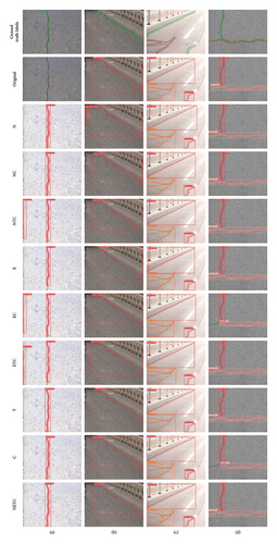
Despite these challenges, the YOLO-NETC model stands out for generating segmentation masks that closely align with the ground-truth annotations, demonstrating superior performance overall. While the model struggles with accurately delineating crack edges under overexposure conditions, it remains the most robust and accurate across the other models in terms of general crack detection.
4.3. Comparative Experiments
The performance of each improved module was confirmed through ablation studies. In order to investigate the effect of different datasets on the improved method (YOLOv8-NETC), each dataset from Section 3.1 was used to train and validate the model, respectively. Meanwhile, each model in Section 3.2 was used to comparatively assess the robustness and sophistication of the improved methods. To ensure the objectivity and fairness of the comparison, all models were constructed on the same system and workstation. In order to quantify the effect of improvements and focus more on proportional changes rather than absolute changes, this section uses a normalization process to calculate the magnitude of the enhancement.
4.3.1. Results for the Crack Type Dataset
In this section, the segmentation results of seven models on the crack type dataset were compared. Table 5 shows the experimental results of PRE, mAP50, REC and F1 for the different models. It was clear that our proposed model achieved the best accuracy. The PRE, mAP50, REC and F1 of YOLOv8-NETC were 78.9%, 77.4%, 77.7% and 78.3%, respectively. The mAP50s were 11%, 70.1%, 17.1%, 75.9%, 12.7%, and 6.5% greater than those of SOLOv2, Cascade Mask R-CNN, CondInst, SparseInst, YOLOv5, and v8, respectively. In terms of the PRE, these values were 2.47% and 0.9% lower and greater than those of YOLOv5 and v8, respectively. In terms of the REC, the values were 19.17% and 5.71% greater than those of YOLOv5 and v8, respectively. In terms of F1, it was 8.43% and 3.32% greater than that of YOLOv5 and v8, respectively. YOLOv8-NETC had a slightly lower PRE than YOLOv5 did, but the PRE was greater than that of YOLOv5 for mAP50, REC and F1. This indicated that YOLOv8-NETC performed better in terms of target localization and matching, especially at higher IoU thresholds, which was crucial for detecting cracks. Notably, all the parameters of the improved model were greater than those of the original model.
| Methods | Instance segmentation | |||
|---|---|---|---|---|
| Precision (%) | mAP50 (%) | Recall (%) | F1 (%) | |
| SOLOv2 | — | 69.7 | — | — |
| Cascade mask R-CNN | — | 45.5 | — | — |
| Condinst | — | 66.1 | — | — |
| Sparseinst | — | 44.0 | — | — |
| YOLOv5 | 80.9 | 68.7 | 65.2 | 72.2 |
| YOLOv8 | 78.2 | 72.7 | 73.5 | 75.8 |
| YOLOv8-NETC (proposed) | 78.9 | 77.4 | 77.7 | 78.3 |
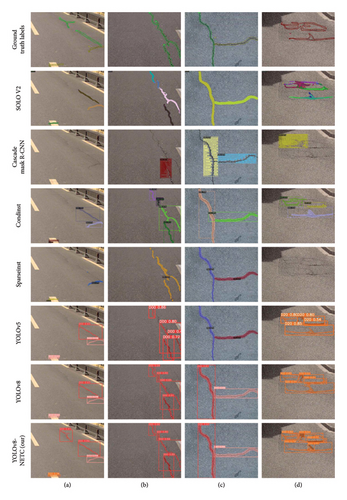
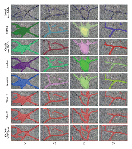
On the crack type dataset, several qualitative comparison results are shown in Figure 13. According to the recognition results of each model on the four images, the SOLOv2 and YOLO series were able to recognize crack skeletons well. However, the recognition result of our proposed YOLOv8-NETC algorithm in Figure 13(a) matches the input image best in terms of crack details. Moreover, comparative models often miss some cracks during recognition. This omission phenomenon was obvious when the models recognized the microcracks and dense cracks in Figures 13(a) and 13(d). In particular, Cascade Mask R-CNN and SparseInst failed to recognize Figures 13(a) and 13(d), respectively. In addition, YOLOv5 also had missing data in continuous crack recognition (Figure 13(b)). The possible reason for the performance degradation of the comparative models is the limitation of the receptive field size and storage. Among the comparative models, the cascade Mask R-CNN achieved the worst segmentation results for very long or complex cracks. Since the model uses a predefined representation of crack shape, it is limited in recognizing irregular cracks. Overall, YOLOv8-NETC achieves satisfactory recognition results on the crack type dataset.
4.3.2. Results for the Crack500 Dataset
To evaluate the generalization ability of the improved model more comprehensively, we conducted experiments on public datasets. Table 6 shows that the improved YOLOv8-NETC algorithm achieved the best accuracy. The mAP50s were 43.81%, 39.93%, 44.61%, 40.69%, 18.42%, and 3.05% greater than those of SOLOv2, Cascade Mask R-CNN, CondInst, SparseInst, and YOLOv5 and v8, respectively. The PRE was 13.95% and 1.85% greater than that of YOLOv5 and v8, respectively. The RECs were 11.97% and 3.09% greater than those of YOLOv5 and v8, respectively. F1 was 12.92% and 2.49% greater than those of YOLOv5 and v8, respectively. Furthermore, combining the results from Section 4.3.1, the YOLO series achieved a higher mAP50 in crack recognition than did the other comparative models. This further demonstrates the practicality of the YOLO series network.
| Methods | Instance segmentation | |||
|---|---|---|---|---|
| Precision (%) | mAP50 (%) | Recall (%) | F1 (%) | |
| SOLOv2 | — | 54.1 | — | — |
| Cascade mask R-CNN | — | 55.6 | — | — |
| Condinst | — | 53.8 | — | — |
| Sparseinst | — | 55.3 | — | — |
| YOLOv5 | 72.4 | 65.7 | 68.5 | 70.4 |
| YOLOv8 | 81.0 | 75.5 | 74.4 | 77.6 |
| YOLOv8-NETC (proposed) | 82.5 | 77.8 | 76.7 | 79.5 |
Figure 14 shows the visualization results of randomly selected images from the Crack500 dataset. It can be clearly seen that the crack predictions of each model basically had the correct orientations. In the columns with closed cracks, (a) and (c), the segmentation by our proposed model was closest to the input image. In contrast, the other models aggressively extended the predicted closed area. Aggressive prediction results might cause additional workload during the inspection process. Moreover, YOLOv5 also missed prediction information at the end of the crack. This misleading prediction was more obvious in the recognition of crossing cracks. According to Figures 14(b) and 14(d), in addition to the improved model, the predictions of each model for the cracks also had shorter, discontinuous, and incorrectly recognized results. Although the improved model performed well overall during the experiment, some problems were still observed. The improved model ignored some shorter cracks, indicating that the model cannot capture the long-range dependency between pixels. An adaptive window size can be used to recognize cracks of different lengths more accurately. In addition, all the models, including the improved model, failed to preserve the actual width of the cracks. This indicates that the fine features are not well distributed, and all the models have room for further improvement in terms of crack width.
4.3.3. Results for the Crack Trueness Dataset
The accuracy advantage of the YOLO series was proven in the above experiments on the crack type dataset and Crack500 dataset. Therefore, to further evaluate the robustness of the model to interference, YOLOv5, YOLOv7, and YOLOv8 were compared with the improved model YOLOv8-NETC. Among the selected models, YOLOv8-NETC, YOLOv5 was the initial frame, YOLOv7 was the previous generation version of the YOLO family, and YOLOv8 was the initial model. The model’s segmentation results are shown in Table 7.
| Methods | Instance segmentation | |||||
|---|---|---|---|---|---|---|
| Precision (%) | mAP50 (%) | Recall (%) | F1 (%) | Model weight (MB) | Parameters | |
| YOLOv5 | 76.5 | 71 | 72.5 | 74.4 | 15.2 | 7,403,816 |
| YOLOv7 | 75.8 | 72.3 | 73.8 | 74.8 | 76.3 | 37,853,264 |
| YOLOv8 | 72.1 | 68.8 | 67.2 | 69.6 | 6.8 | 3,258,649 |
| YOLOv8-NETC (proposed) | 77.1 | 74.7 | 74.5 | 75.8 | 6.4 | 3,051,691 |
On the crack trueness dataset, the improved model YOLOv8-NETC demonstrated superior performance, showing significant improvements across all key metrics compared to the traditional YOLOv5, YOLOv7, and YOLOv8 models. Specifically, YOLOv8-NETC achieved Precision, mAP50, Recall, and F1 scores of 77.1%, 74.7%, 74.5%, and 75.8%, respectively, highlighting its exceptional ability to balance precision and recall. Compared to the stable-performing YOLOv5, YOLOv8-NETC improved mAP50 by approximately 5.2% and Recall by about 2.8%, respectively, while maintaining a higher F1 score. This indicates that the model not only detects cracks more effectively but also reduces the miss-detection rate. When compared to the larger model YOLOv7, YOLOv8-NETC achieved approximately a 1.3% increase in F1 score, all while benefiting from a lightweight architecture that significantly reduces the number of parameters and computational complexity. In contrast to the baseline YOLOv8, YOLOv8-NETC exhibited more noticeable improvements across all metrics, particularly in mAP50 and Recall, which were enhanced by approximately 8.6% and 10.9%, respectively. This demonstrates that the improved modules are better adapted to the diverse features of cracks. In conclusion, the comprehensive performance advantages of YOLOv8-NETC validate its potential in crack segmentation tasks and provide a reliable solution for efficient crack detection in practical engineering applications.
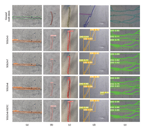
The visualization results of different models on the real-world crack dataset are presented in Figure 15. For the detection of expansion joints in image (a), YOLOv5 to YOLOv8 all exhibit missing detections along the edges of the expansion joints. Notably, YOLOv8 demonstrates a recurring issue of duplicate detections. Among all models, YOLOv8-NETC achieves the most complete detection of the expansion joints. In the detection of tree branches in image (b), all models perform well. Compared to expansion joints, the color contrast between the tree branches and the background is more pronounced, making it easier for the models to identify the targets. However, in the detection of water stains and horizontal cracks, YOLOv8 continues to exhibit duplicate detections for single targets as well as false detections on manhole covers. The likely reasons for these issues are insufficient multiscale feature fusion in the segmentation module or the loss function’s inability to effectively penalize duplicate predictions. The improved YOLOv8-NETC successfully addresses these problems, providing more accurate and reliable detection results.
5. Conclusions and Outlook
- 1.
Based on ablation studies, compared to the Baseline, YOLOv8-NETC achieved a 6.5% improvement in mAP50, a 6.1% average reduction in MW and parameters, and an 8.5% increase in FPS. Among all modules, YOLOv8-NETC offers good accuracy while maintaining high speed and low memory usage, making it more advantageous for practical applications.
- 2.
Based on comparison experiments, YOLOv8-NETC achieved the highest mAP50 of 77.4% and 77.8% on the crack type dataset and Crack500 dataset, respectively. Moreover, the accuracy advantage of YOLO series models was validated on these datasets.
- 3.
On the trueness dataset, YOLOv8-NETC had the lowest weight and P, at 6.4MB and 3.05 million, respectively, with the highest mAP50 of 74.7%. YOLOv8-NETC demonstrated better storage efficiency and robustness compared to other models, showing potential for applications on portable edge devices.
Despite the promising performance of the proposed method in this study, several directions can be explored and improved upon in future work. Specifically, future work can focus on the following four aspects: (1) Enhancing model robustness: Further improving the robustness of the proposed model by utilizing data augmentation and regularization techniques. (2) Balancing accuracy and efficiency: Future work could explore increasing the model’s complexity to improve accuracy, while carefully balancing the tradeoff between model size and inference speed. (3) Detection of fine and complex cracks: Despite improvements in model accuracy, detecting fine and complex cracks remains challenging. Techniques such as multiscale feature extraction and more efficient patch merging strategies can help enhance the performance for small-scale cracks. (4) Real-time processing: Optimizing the model for real-time applications by improving computational efficiency, possibly through model pruning or hardware acceleration, would address hardware constraints.
Conflicts of Interest
The authors declare no conflicts of interest.
Funding
The research in this paper was financially supported by the 2022 Research Project of Xinjiang Key Laboratory of Hydraulic Engineering Security and Water Disasters Prevention (ZDSYS-YJS-2022-11), the Central Government-Guided Funds for Regional Science and Technology Development (No. ZYYD2024CG20), and the National Natural Science Foundation of China (No. 52378152). Their support was gratefully acknowledged.
Acknowledgments
The research in this paper was financially supported by the 2022 Research Project of Xinjiang Key Laboratory of Hydraulic Engineering Security and Water Disasters Prevention (ZDSYS-YJS-2022-11), the Central Government-Guided Funds for Regional Science and Technology Development (No. ZYYD2024CG20), and the National Natural Science Foundation of China (No. 52378152). Their support was gratefully acknowledged.
Open Research
Data Availability Statement
The data that support the findings of this study are available from the corresponding author upon reasonable request.


