BNN-LSTM-DE Surrogate Model–Assisted Antenna Optimization Method Based on Data Selection
Abstract
The use of surrogate models in assisting evolutionary algorithms for antenna optimization has achieved significant research outcomes. The construction of surrogate model primarily depends on two aspects; one is the selection of datasets, and the other is the model’s structure and performance. This paper proposes a novel dataset selection method aimed at enhancing the performance of the constructed surrogate model. Additionally, based on Bayesian neural network (BNN) and leveraging the advantages of handling sequence data with long short-term memory (LSTM), a BNN-LSTM surrogate model is introduced. After training, this surrogate model is used as the fitness evaluation function, enabling optimization design based on differential evolution (DE) algorithm. Experimental validations are conducted using the optimizations of a dual-frequency slotted patch antenna and a rectangular cut-corner ultrawideband antenna as examples. Results demonstrate that the proposed surrogate model exhibits high accuracy, providing a guidance for antenna optimization.
1. Introduction
During antenna optimization design, global optimization (GO) algorithms typically require full-wave electromagnetic (EM) simulation software to evaluate the performance of the antenna. Therefore, a considerable amount of calling full-wave EM simulation is needed in the optimization process to obtain the optimal design, making the optimization cost unacceptable. To replace computationally expensive full-wave EM simulation software, machine learning (ML) methods have been widely introduced into the field of antenna optimization design. Trained ML-based surrogate models can replace full-wave EM simulation software to predict antenna performance [1]. The prediction time of surrogate models can be almost negligible compared to full-wave EM simulation time. Therefore, the main computational cost of using this method lies in establishing the dataset and training process, significantly reducing the time spent on the calling full-wave EM simulation software during optimization. Nakmouche et al. [2] used artificial neural network (ANN) as surrogate models for optimizing dual-band antennas with H-slot defect grounding structures. Dong, Li, and Wang [3] employed particle swarm optimization (PSO) to enhance the accuracy of radial basis function neural network (RBFNN) in antenna modeling. They combined the optimized RBFNN with multiobjective evolutionary algorithms for optimization design of multiobjective antenna with multiparameter structures. Gao, Tian, and Chen [4] proposed a semisupervised collaborative training algorithm based on Gaussian processes (GPs) and support vector machine (SVM) for antenna modeling. They validated the proposed algorithm’s effectiveness in replacing time-consuming EM simulation software through optimizations of benchmark functions and Yagi microstrip antennas. Koziel and Ogurtsov [5] used space mapping as the optimization engine and response surface approximation as the surrogate model to optimize the antennas. Additionally, ML methods such as Kriging models [6], polynomial regression [7], and decision tree regression [8] are also used as surrogate models to assist in antenna optimization design.
Long short-term memory (LSTM) network is a type of specialized recurrent neural network (RNN) that exhibits clear advantages in handling time series data. Time series refers to a series of data points or observations arranged in chronological order. In time series analysis, time typically serves as the independent variable, while the observations serve as the dependent variable. The chronological order of such data is crucial for analysis because it reflects potential temporal correlations and trends among data points. LSTM networks have been widely applied in various domains such as stock market price prediction [9], forecasting of oil production [10], and natural language processing [11]. In the field of antenna optimization, LSTM can also leverage its advantages because the dataset used to construct surrogate models can be viewed as time series data, with labels arranged in order of frequency.
Bayesian neural networks (BNNs) differ from traditional deterministic ANNs like multilayer perceptron (MLP) by incorporating Bayesian statistical concepts and methods into the modeling process. They introduce Bayesian inference for prediction, providing not only predicted label values but also estimates of uncertainty associated with the predictions. Liu et al. [12] explored the advantages of BNNs over GP and applied them in combination with differential evolution (DE) algorithms to antenna optimization design, demonstrating the effectiveness of BNNs as surrogate models. This paper combines BNN with LSTM, named Bayesian neural network-long short-term memory (BNN-LSTM) surrogate, to imbue the surrogate model with model uncertainty, thereby integrating the advantages of LSTM in time series prediction with the BNN’s ability to provide statistically grounded estimates of prediction uncertainty.
It is well known that the selection of the dataset is crucial for constructing surrogate models. For a larger parameter optimization range, it is necessary to sample more parameter combinations in the optimization space to ensure the fitting effectiveness of the surrogate model, which increases the cost of dataset construction. Conversely, a smaller parameter optimization range may lead optimization algorithms to trap in local optima when optimizing parameters. Latin hypercube sampling (LHS) [13, 14] is widely used for initial dataset selection. However, although LHS can comprehensively cover samples across the parameter optimization space, achieving precise predictions throughout the entire parameter space still requires a large number of parameter combinations, thereby increasing computational costs. In the field of antenna optimization design, due to spatial constraints, the optimal parameter space is typically not large. Therefore, our goal is to identify this space and ensure the surrogate exhibits good modeling performance.
This paper introduces a novel surrogate model by combining LSTM network and BNN into the field of antenna optimization. It also proposes a new method for generating datasets aimed at reducing the optimization space for antenna parameters. Within this defined space, the surrogate is constructed to enhance the accuracy of antenna modeling. The remainder of this paper is organized as follows. Section 2 provides a brief overview of related works. Section 3 details the proposed methods. Section 4 demonstrates the effectiveness of the method through antenna modeling and optimization cases. Finally, Section 5 concludes the paper and outlines future research directions.
2. Related Works
2.1. LSTM
RNNs are a type of ANNs specifically designed to handle sequential data. Unlike traditional feedforward ANNs, RNNs possess the ability to remember sequential data [15]. LSTM is a variant of RNNs initially designed to address the issue of long-term dependencies inherent in RNNs [16]. Compared to traditional RNNs, LSTM introduces three gates: the input gate, forget gate, and output gate, along with a cell state. These structures enable LSTM to better handle long-term dependencies within sequences. The structure is illustrated in Figure 1, where Circle 1 represents the forget gate, Circle 2 the input gate, Circle 3 the output gate, and Circle 4 the cell state update process.
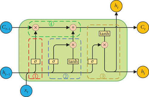
Here, ft represents the output of the forget gate, σ denotes the Sigmoid function, Wf, bf are, respectively, the weight matrix and bias term of the forget gate, and [ht−1, xt] denotes the concatenation of the previous cell output and the current input.
Here, it represents the output of the input gate, Wi, bi are the weight matrix and bias of the input gate, respectively, is the candidate cell state, and Wc, bc are the weight matrix and bias of the candidate cell state, respectively.
Here, ot represents the output of the output gate, Wo and bo are, respectively, the weight matrix and bias of the output gate, and ht is the output of the LSTM unit.
LSTM effectively addresses the gradient and long-term dependency issues in traditional RNNs by introducing three gates and a cell state, thereby providing significant advantages and practical value in sequence modeling and prediction tasks.
2.2. BNNs
BNNs, in essence, can be understood as regularizing ANNs by introducing uncertainty into the weights, akin to integrating predictions over an infinite set of ANNs sampled from a certain weight distribution. Traditional ANNs have fixed weights after training. In contrast, BNNs consider weights to follow a Gaussian distribution with mean μ and variance δ, and each weight follows a distinct Gaussian distribution [17], as illustrated in Figure 2.
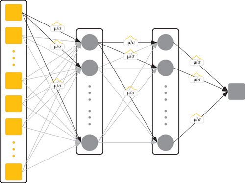
During prediction, BNNs sample from each Gaussian distribution to obtain weight values, which is equivalent to traditional ANN. After multiple sampling predictions and averaging, the predicted value of BNNs can be obtained, which means BNNs are also equivalent to an ensemble model.
2.3. DE Algorithm
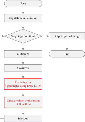
DE algorithm is a stochastic heuristic search algorithm based on population differences. It was proposed by Storn and Price [19] in 1997 to solve Chebyshev polynomial problems. Due to its characteristics of simplicity, robustness, and fast convergence [20], it has been widely applied in various fields. DE algorithm performs mutation, crossover, and selection operations based on the differential vector between parent individuals. The basic idea is to start from a randomly generated initial population, creating a new individual by weighted addition of the vector difference between any two individuals in the population and the sum with a third individual according to certain rules. The new individual is then compared with a predetermined individual from the current population. If the fitness value of the new individual is better than that of the compared individual, the new individual replaces the old one in the next generation; otherwise, the old individual is retained. Through continuous iterative computation, DE algorithm preserves good individuals, eliminates poor individuals, and guides the search process towards the optimal solution.
In the equation, xr1, xr2, and xr3 are three randomly selected distinct individuals from the current gth generation population, and they should not be the same as the target individual, that is, i ≠ r1 ≠ r2 ≠ r3. vi(g) represents the ith mutated individual generated in gth generation, where F is the mutation factor.
Here, uij(g) represents the jth component of the ith crossover individual generated in gth generation, CR ∈ [0, 1] is the crossover factor, and jrand is a random integer from [1, 2, ⋯, D], ensuring that at least one component of the trial individual after crossover is provided by the mutated individual.
3. The Proposed Method
3.1. Data Selection
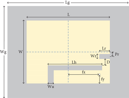
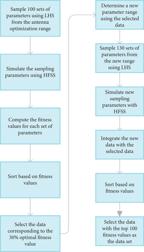
In order to clearly demonstrate the method proposed in the paper, we take modeling the frequency characteristics of a dual-frequency slotted patch antenna shown in Figure 3 as an example. The design requires the antenna to exhibit dual resonances within the frequency range of 1.5–3 GHz. To comprehensively cover the antenna parameter space, LHS is employed to sample 100 sets of parameters from the multidimensional parameter space. HFSS simulation software is used to obtain the frequency characteristic for each set of parameters. Leveraging the idea of fitness evaluation for offspring selection in genetic algorithm (GA), an appropriate fitness function is initially defined based on the antenna design requirements, and fitness values are calculated based on the corresponding frequency characteristic of the antenna. By comparing the fitness values of various antenna parameters and sorting them from smallest to largest (where smaller fitness value indicates better antenna performance in this study), antenna parameters with fitness values in the top 30% are selected as the new dataset. This dataset is analyzed to determine the maximum and minimum values of each antenna parameter, establishing a new parameter range to narrow down the antenna optimization scope and thereby enhance the accuracy of the surrogate model. When the range of antenna modeling parameters has been reduced, the dataset size is insufficient to meet the requirements for surrogate model construction at this stage. Therefore, an additional 130 sets of samples are obtained using LHS within the new modeling parameter range, and HFSS simulations are conducted to obtain the dataset. The newly obtained dataset is combined with the dataset selected from the first round, totally 160 sets of data. Subsequently, the same method as before is used for the second round of selection, resulting in the selection of the top 100 sets of antenna. The primary purpose of the first selection is to reduce the modeling parameter range, while the second selection is aimed at not only further narrowing down the antenna optimization scope but also acquiring sufficient training data for training the surrogate model. Eighty samples are randomly selected from these 100 datasets as the training set for training the antenna surrogate model, while the remaining 20 samples serve as the test set to validate the performance of the antenna surrogate model. The process flowchart of the data selection method is shown in Figure 4.
3.2. The BNN-LSTM Surrogate Model
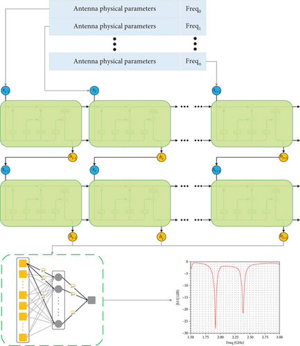
LSTM networks possess the ability of LSTM, offering significant advantages in predicting time series data. In antenna simulation, the frequency characteristic ∣S11∣ of an antenna can be viewed as a time series, where frequency points represent time steps, and the ∣S11∣ values corresponding to these frequency points can be considered as labels. However, using only frequency points as input does not meet the requirements for constructing a surrogate model because different parameters’ combination also affects the antenna’s performance. Therefore, in this study, both antenna dimensional parameters and frequency points are used together as input features for the LSTM network to model the antenna’s performance. Thus, at each step, the input consists of combinations of antenna parameters and frequency points, while the output is the corresponding ∣S11∣ value at the frequency point. In this study, the LSTM model employs a two-layer structure, in where the first layer has an input dimension equal to the feature dimension with an output set to 64 dimensions, and the second layer also has an input of 64 dimensions and outputs 64 dimensions.
Following LSTM, a single-layer BNN integrates the features computed from the LSTM layer, mapping them into the sample label space. Utilizing the predictive uncertainty provided by the BNN model guides DE algorithm more effectively to find the optimal parameters of the antenna. This forms a hybrid surrogate model of LSTM and BNN, named BNN-LSTM model in this paper. This layer has an input dimension of 64, which corresponds to the output of the final layer of LSTM. The output dimension is 1, representing the predicted ∣S11∣ value of the antenna at the corresponding antenna parameters and frequency point. Figure 5 illustrates the process of the surrogate model predicting the ∣S11∣ parameters of antenna.
3.3. Optimization Using DE Algorithm Based on the Proposed BNN-LSTM Surrogate Model
Here, ylcb(x) represents the predicted LCB, denotes the predicted mean value, and ω is a constant used to control the confidence level and set to 2 in this study. represents the prediction uncertainty. Figure 6 illustrates the optimal process of antennas by combining DE algorithm with the trained surrogate models, called as the BNN-LSTM-DE (Bayesian neural network-long short-term memory-differential evolution) algorithm in the paper.
4. Experiment and Discussion
4.1. Evaluation Metrics
Here, m represents the sample size, yi denotes the true value of the ith observation, represents the model’s predicted value for the ith observation, and denotes the average value of all observations.
4.2. Optimization Design of Dual-Frequency Slotted Patch Antenna
| Optimized parameters | Initial parameter optimization space S0 (mm) | The first selection | The second selection | ||
|---|---|---|---|---|---|
| The parameter optimization space S1 (mm) | The reduction percentage (relative to space S0) | The parameter optimization space S2 (mm) | The reduction percentage (relative to space S1) | ||
| W | [65, 70] | [65.2, 69.94] | 5.2% | [65.2, 69.8] | 2.9% |
| L | [55, 70] | [55, 68.65] | 9.0% | [55, 68.6] | 0.4% |
| WR | [1, 8] | [1.32, 7.9] | 6.0% | [1.32, 7.8] | 1.5% |
| WU | [1, 8] | [1.17, 6.84] | 19.0% | [1.20, 6.8] | 1.2% |
| LR | [1, 10] | [1.06, 9.87] | 2.1% | [1.06, 9.8] | 0.8% |
| PR | [0, 5] | [0.08, 4.97] | 2.2% | [0.15, 4.9] | 2.9% |
| LH | [40, 54] | [40.54, 53.93] | 4.4% | [40.6, 53] | 7.4% |
| D | [1, 5] | [1, 4.87] | 3.3% | [1.2, 4.86] | 5.4% |
Data collection is conducted using HFSS simulation software, and the sweep range is 1.5–3 GHz with a step size of 10 MHz. This allows for a comprehensive observation of the antenna’s frequency characteristics and their variations within the sweep range.
In Table 1, the initial antenna parameter optimization space is denoted as S0, and the space is denoted as S1 after first selection and S2 after second selection. From Table 1 we know, after the first selection, the optimization range of parameter space S1 decreased by an average of approximately 6.4% compared to the initial parameter space S0. After the second selection, the optimization range of parameter space S2 decreased by an average of approximately 2.81% compared to parameter space S1. The largest reduction in optimization range occurs after the first selection, primarily because the first selection is aimed at finding the optimal space, thus retaining fewer parameter sets than the second selection, mainly to gather sufficient effective data for training the model. The data selection process utilizes the selection principle of GA, wherein the fitness function is used to select datasets. After data selection, the remaining data are those with higher fitness value. The increase of population fitness value generally accompanies the reduction of optimization space, thereby enhancing the accuracy of the surrogate model.
Table 2 presents the modeling performance of the BNN-LSTM model trained using different datasets in this study. To ensure equal computational costs across different models, total 230 simulations in HFSS is set to each model. The difference lies in the method of dataset selection. Model M0 is trained using 230 samples obtained through LHS within the initial optimization range S0. Model M1 obtains 100 samples through LHS firstly within the initial optimization range S0 and then selects the top 30% samples according to fitness value, thus resulting in 30 samples. After the first selection, additional 130 samples are obtained through LHS within the new optimization range S1, and then, we have 160 samples for training. Model M2 is trained using the top 100 samples with high fitness value selected from the 160 samples of model M1. Each model’s training set consisted 80% of its total data, with the remaining 20% reserved for testing. From Table 2, it can be seen that model M0, trained using the initial dataset, performs the worst. Next is model M1, trained with one selection and resampling process. Model M1 shows an improvement of approximately 4.1% in R2 and reductions of 17.3% and 13.0% in MSE and MAE, respectively, compared to model M0. This indicates a significant improvement in model M1’s performance over model M0. However, considering the magnitudes of R2, MSE, MAE, and other indicators, model M1 is still inadequate as a trustworthy surrogate model. The best-performing model is M2, trained with data that underwent two selection processes. Model M2 exhibits an increase in R2 by 9.5% compared to model M1, with reductions in MSE and MAE by 51.4% and 25.4%, respectively. Model M2 shows a significant performance improvement over model M1, demonstrating the effectiveness of data selection method. Considering the significant differences in parameters within the larger optimization range S0, this inevitably increases the modeling difficulty, hence resulting in the poorer performance metrics of model M0. Despite the smaller training dataset S1 compared to model M0, the parameter training range of model M1 is reduced, leading to improved performance. The same applies to model M2.
| Metrics | Model M0 | M1 relative to M0 | Model M1 | M2 relative to M1 | Model M2 |
|---|---|---|---|---|---|
| MSE | 1.907 | 17.3% | 1.577 | 51.4% | 0.766 |
| R2 | 0.812 | 4.1% | 0.845 | 9.5% | 0.925 |
| MAE | 0.638 | 13.0% | 0.555 | 25.4% | 0.414 |
In Table 3, the proposed LSTM-BNN surrogate model is compared with several commonly used ML surrogate models including ANN, K-nearest neighbor, and decision tree. All trained on the same dataset as Model M2. As shown in Table 3, the LSTM-BNN outperforms the other three models in terms of MSE, MAE, and R2, due to LSTM’s unique advantages in handling sequential data, while the BNN layer naturally integrates multiple models, enhancing predictive performance. This demonstrates the effectiveness of the proposed surrogate model for antenna modeling.
| Model | MSE | MAE | R2 |
|---|---|---|---|
| Artificial neural network | 2.744 | 0.660 | 0.446 |
| K-nearest neighbor | 1.984 | 0.461 | 0.805 |
| Decision tree | 3.452 | 0.423 | 0.660 |
| LSTM-BNN | 0.766 | 0.414 | 0.925 |
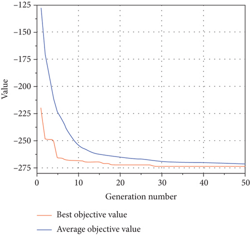
Figure 7 depicts the optimal fitness function curve and the population average fitness curve when optimizing antenna parameters using the trained surrogate model M2 combined with DE algorithm. It can be observed that both the average population fitness curve and the optimal fitness function curve show continuous decreases. The decreasing trend of the average population fitness function indicates that the optimization algorithm successfully guides the population towards more optimal solution direction, while the decrease in the optimal population fitness function curve indicates that the optimization algorithm is able to find better solutions during the optimization process. The final flattening of both curves indicates that the optimization algorithm has converged, gradually finding the optimal solution within the optimization space.
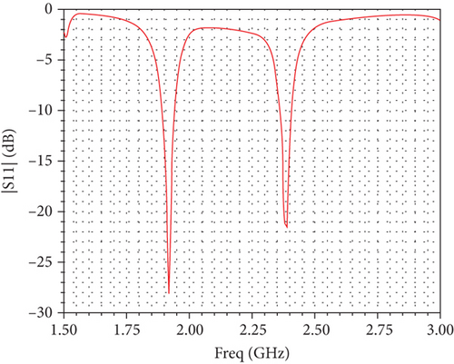
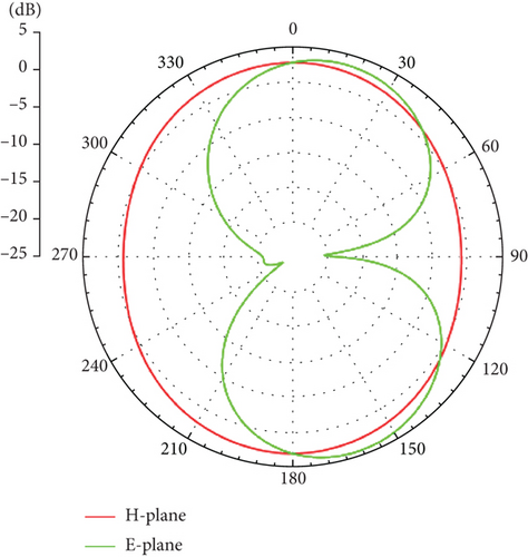
The optimized parameters of the dual-frequency slotted patch antenna using the proposed algorithm in this paper are shown in Table 4. Figure 8 illustrates ∣S11∣ simulated by HFSS software based on the optimal parameters. Figure 9 presents the antenna radiation pattern at 1.9 and 2.4 GHz. From Figure 8, it can be observed that the ∣S11∣ values of the antenna at 1.9 and 2.4 GHz are both less than −10 dB, meeting the design requirements, which demonstrates the effectiveness of the proposed BNN-LSTM-DE algorithm for antenna optimal design.
| Parameters | W | L | WR | WU | LR | PR | LH | D |
|---|---|---|---|---|---|---|---|---|
| Value (mm) | 67.41 | 57.27 | 1.44 | 5.19 | 7.26 | 4.88 | 53.00 | 4.10 |


4.3. Optimization Design of Rectangular Cut-Corner Ultrawideband (UWB) Antenna
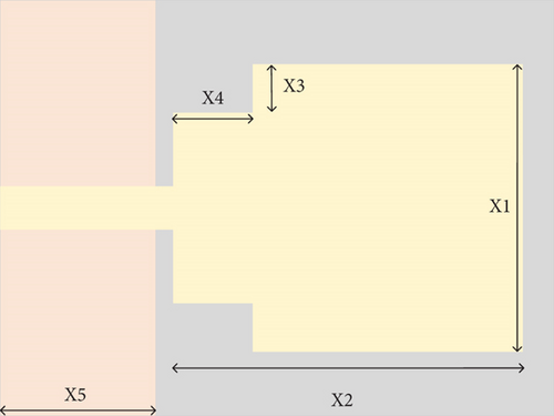
Example 2 is the rectangular cut-corner UWB antenna [23]. As we all know, traditional rectangular patch antennas have a relatively narrow operating bandwidth. In order to increase it, two symmetrical rectangular slots are cut at both ends of the patch, shown in Figure 10. The parameters to be optimized for the antenna are set as [X1, X2, X3, X4, X5], and the corresponding search space is indicated in the initial parameter optimization space S0 shown in Table 5. The antenna uses an FR4 dielectric substrate measuring 31 mm in length, 24 mm in width, and 1 mm in thickness, fed by a microstrip line that is 10 mm long and 2 mm wide, with a grounded plane on the back.
| Optimized parameters | Initial parameter optimization space S0 (mm) | The first selection | The second selection | ||
|---|---|---|---|---|---|
| The parameter optimization space S1 (mm) | The reduction percentage (relative to space S0) | The parameter optimization space S2 (mm) | The reduction percentage (relative to space S1) | ||
| X1 | [12, 18] | [12, 17.93] | 1.1% | [12.08, 17.93] | 1.3% |
| X2 | [18, 21] | [18.1, 20.98] | 4.0% | [18.11, 20.97] | 0.7% |
| X3 | [1, 5] | [1.21, 4.98] | 5.8% | [1.31, 4.73] | 9.3% |
| X4 | [1, 5] | [1.14, 4.86] | 7.0% | [1.17, 4.81] | 2.2% |
| X5 | [5, 10] | [7.85, 9.98] | 57.4% | [7.89, 9.98] | 1.9% |
Here, f1 = 2 GHz, f2 = 3.1 GHz, f3 = 10.6 GHz, and f4 = 12 GHz; |S11(f)| represents the reflection loss magnitude of the antenna at frequency f.
The data is also collected using HFSS simulation software with a frequency range from 2 to 12 GHz and a sweep step size of 100 MHz. In Table 5, the optimization space S1 is reduced by approximately 15.1% on average compared to the initial optimization space S0. The optimization space S2 is reduced by approximately 3.08% on average compared to optimization space S1. This result further confirms the effectiveness of the data selection method. As shown in Table 6, the model M0 trained on the initial dataset has the worst performance. The model M1, trained on the dataset after one selection, performs slightly better. R2 of model M1 improved by approximately 3.3% compared to model M0, while the MSE and MAE decreased by 5.0% and 15.2%, respectively. This indicates that model M1 shows significant improvement over model M0. The best-performing model is M2, trained on the dataset after two selection processes. This model achieved an 1.3% increase in R2 compared to model M1, with reductions in MSE and MAE of 6.0% and 1.2%, respectively. These results demonstrate the effectiveness of the proposed method in improving model prediction performance with the same consuming computing time.
| Metrics | Model M0 | M1 relative to M0 | Model M1 | M2 relative to M1 | Model M2 |
|---|---|---|---|---|---|
| MSE | 2.976 | 5.0% | 2.826 | 6.0% | 2.658 |
| R2 | 0.880 | 3.3% | 0.909 | 1.3% | 0.921 |
| MAE | 1.065 | 15.2% | 0.903 | 1.2% | 0.892 |
In Table 7, different surrogate models are used to model the rectangular cut-corner UWB antenna, and the datasets are the same as those used for training model M2. As shown in Table 7, MSE, MAE, and R2 of the LSTM-BNN model outperform those of the other three models. This indicates the effectiveness of the proposed surrogate model for antenna modeling.
| Model | MSE | MAE | R2 |
|---|---|---|---|
| Artificial neural network | 4.018 | 1.247 | 0.863 |
| K-nearest neighbor | 15.037 | 2.515 | 0.550 |
| Decision tree | 17.118 | 2.390 | 0.488 |
| LSTM-BNN | 2.658 | 0.892 | 0.921 |
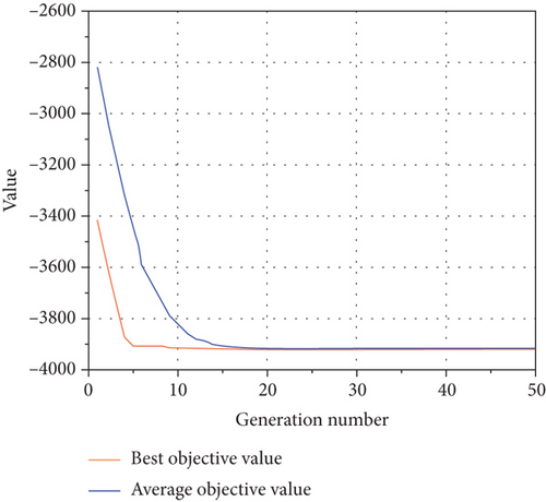
Figure 11 shows the trends of the optimal fitness curve and the average fitness curve of the population during the optimization of the rectangular cut-corner UWB antenna. As seen in Figure 11, both curves gradually decrease and stabilize with the increase in evolutionary generations, indicating that the optimization algorithm is converging and ultimately finding the optimal solution within the optimization space.
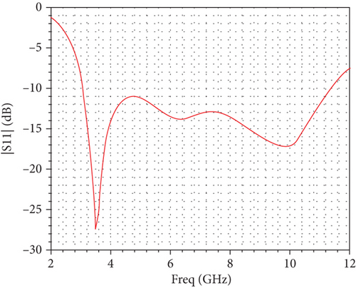
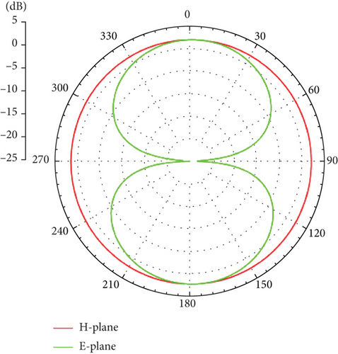
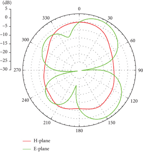
The parameter dimensions of the rectangular cut-corner UWB antenna optimized based on the proposed algorithm are shown in Table 8. Figure 12 illustrates the ∣S11∣ values obtained from HFSS using these parameters. As seen in Figure 12, the antenna bandwidth fully covers the UWB operating frequency range of 3.1–10.6 GHz. Figure 13 presents the two-dimensional radiation patterns at frequencies of 3, 6, and 9 GHz, where the green curve represents the E-plane and the red curve represents the H-plane. As shown in Figure 13, the antenna radiation pattern in the H-plane is approximately circular, while the E-plane resembles the shape of the digit “8.” Some distortion occurs at higher frequencies, but it still meets the expected requirements. This example further demonstrates the effectiveness of the proposed algorithm for antenna optimization.
| Parameters | X1 | X2 | X3 | X4 | X5 |
|---|---|---|---|---|---|
| Value (mm) | 17.92 | 20.97 | 2.98 | 4.81 | 9.07 |
5. Conclusion
This paper integrates LSTM network with BNN as a novel surrogate model for EM optimization. Simultaneously, we propose a new data selection method to enhance the modeling capability of the surrogate model. Following the EM optimization is complemented by DE algorithm based on the trained surrogate model. The paper validates the proposed algorithm by optimizing the dual-frequency slotted patch antenna and the rectangular cut-corner UWB antenna. Experimental results demonstrate that the data selection method significantly enhances the modeling effectiveness. The optimal results also confirm the outstanding performance of the proposed algorithm. Future research will include modeling and optimizing antennas with multiobjection including pattern, gain, and reflection.
Conflicts of Interest
The authors declare no conflicts of interest.
Author Contributions
Jinlong Sun: conceptualization, methodology, software, investigation, formal analysis, writing–original draft; Yubo Tian: funding acquisition, resources, supervision, writing–original draft, writing–review and editing; Zhiwei Zhu: data curation, writing–original draft. All authors agree to be accountable for the content and conclusions of the article.
Funding
This work was supported by the Natural Science Foundation of Guangdong Province of China under Grant No. 2023A1515011272, the Tertiary Education Scientific Research Project of Guangzhou Municipal Education Bureau of China under No. 202234598, the Special Project in Key Fields of Guangdong Universities of China under No. 2022ZDZX1020, and the Engineering Technology Center of Guangdong Province Universities of China under No. 2022GCZX004.
Acknowledgments
This work was supported by the Natural Science Foundation of Guangdong Province of China under Grant No. 2023A1515011272, the Tertiary Education Scientific Research Project of Guangzhou Municipal Education Bureau of China under No. 202234598, the Special Project in Key Fields of Guangdong Universities of China under No. 2022ZDZX1020, and the Engineering Technology Center of Guangdong Province Universities of China under No. 2022GCZX004.
Open Research
Data Availability Statement
The data that support the findings of this study are available from the corresponding author upon reasonable request.


