Autonomous UAV Path Optimization Using Genetic and Multiobjective Evolutionary Algorithms for Effective Data Retrieval in Cache-Enabled Mobile Ad-Hoc WSNs
Abstract
Collecting data from nodes in mobile ad hoc wireless sensor networks is a persistent challenge. Traditional methods rely on specialized routing protocols designed for these environments, with research often aimed at improving efficiency in terms of throughput and energy consumption. However, these improvements are often interconnected, where gains in one area can lead to compromises in another. An alternative approach uses unmanned vehicles (UVs), particularly unmanned aerial vehicles (UAVs), due to their adaptability to various terrains. Unlike traditional methods, UAVs can collect data directly from mobile nodes, eliminating the need for routing. While most existing research focuses on static nodes, this paper introduces a multiple objective evolutionary approach “Strength Pareto Evolutionary Algorithm for Dynamic UAV Paths” (SPEA-DUP) for UAV data collection that predicts the future positions of caching-enabled mobile ad hoc wireless sensor network nodes. SPEA-DUP aims to maximize encounters with nodes and gather the most valuable data in a single trip. The proposed technique is tested across different simulation scenarios, movement models, and parameter configurations and is compared to our genetic algorithm ‘Genetic Algorithm-Aerial Paths’ (GA-AP) counterpart to evaluate its effectiveness.
1. Introduction
Wireless sensor networks (WSNs) and mobile ad hoc networks (MANETs) are widely utilized across various domains, including environmental monitoring, military operations, vehicular communications, and animal tracking [1–6]. The application of these networks is domain-specific, employing diverse sensors for tasks such as humidity and seismic monitoring, collision detection, and physiological measurements like pulse and temperature. In WSNs, sensor nodes are statically deployed to gather and relay data to a central destination for analysis. Conversely, MANETs consist of mobile nodes that form temporary, self-configuring networks during deployment. These nodes are often resource-constrained, with limited processing capabilities and small battery capacities, making energy efficiency a major design consideration. Traditionally, data transmission relies on routing protocols that forward packets from source to destination, introducing overhead and increasing energy consumption. Despite numerous optimization efforts in routing strategies [7–9], fundamental trade-offs persist. As an alternative, this study proposes the use of unmanned aerial vehicles (UAVs) to periodically retrieve data from caching-enabled nodes, effectively eliminating the need for routing and thereby reducing energy expenditure.
Multiobjective theory is used when there is a need of accomplishing multiobjectives usually in terms of optimization rather than having just one. For instance, deciding the best path between two cities is quite easy when the standard to judge that is set to distance. In that case, the path having the shortest distance between two cities can easily be termed as the most optimum path. However, if the standard is reliant on more than one characteristic, things start to get a bit more complex. Several multiobjective evolutionary algorithms (Table 1) have been proposed over the past few years.
Niched Pareto genetic algorithm (NPGA) [10] is an MOEA that introduces the combination of tournament selection and Pareto dominance. Two random individuals are selected for competition and are later compared against a random set of individuals. Out of the two individuals, a winner of the tournament is decided if no other individual from the set dominates it. If both individuals end up being dominated or vice versa, the concept of sharing is adapted. Sharing handles the solution density problem on the Pareto front. A higher count of neighbors in an individual’s vicinity results in a penalty, decreasing the fitness value of that individual. Initially, the distance between the solutions is determined through the Euclidean distance and later compared against a predefined sharing value to impose penalties. For the two competitors, the individual with minimum individuals in the niche is selected.
Pareto envelope-based selection algorithm (PESA) [17] maintains a separate archive alongside the main population to store nondominated solutions iteratively. Upon completion, solutions from the final iteration constitute the Pareto optimal front. It employs squeeze-factor and hyper-boxes to diversify the solution set and aid parent selection. Virtual grids map the solution space, recording observations where grids contain multiple solutions. Each solution in such grids gains a squeeze factor equivalent to the grid’s solution count. If the archive exceeds a reasonable size, solutions are removed based on higher squeeze-factor values. Reproduction selects individuals with the lowest squeeze-factor values. Li et al. [18] enhanced PESA with three key improvements: retention of boundary solutions, streamlined archive updates, and enhanced convergence by discarding the worst individuals in densely populated grids.
Pareto archived evolution strategy (PAES) [16] works by selecting a randomly generated solution, evaluating the fitness on it and creating a copy of the same solution. The copy is mutated before the original and the copy are compared with respect to dominance. If one dominates the other, it is taken as the nondominated solution else if dominance remains undetermined, the solution is compared with an existent set of nondominated solutions from the previous steps. If still the dominance does not get determined, the solution with the least crowding is chosen.
Vector evaluated genetic algorithm (VEGA) [19] is a type of MOEA that divides the total population into multiple equal parts. A random part is filled with randomly chosen individuals after which the population is later shuffled, crossed, and mutated. A set of individuals representing the most optimal solutions is selected based on an inferiority concept. An individual is termed as an inferior individual if for any other individual, considering the aim of minimization, the second individual for one objective is less than the first and for another objective it is at maximum, equivalent to the first. The noninferior members are then presented as the solution set covering the Pareto optimal front.
Multiobjective evolutionary algorithm based on decomposition (MOEA/D) [20] decomposes the problem into scalar optimization subproblems, each addressing an independent aspect of the overall objective space. It evolves populations for each subproblem, retaining the best solutions in each generation to update subsequent iterations. Techniques such as weighted sum, Tchebycheff, and boundary intersection are employed based on problem characteristics. Objective normalization ensures fair comparison and optimal solution generation across different objectives, while exploiting neighborhood relations among subproblems drives exploration and convergence to diverse high-quality solutions. By optimizing individual subproblems rather than the entire multiobjective problem, MOEA/D reduces computational complexity, making it effective for high-dimensional or large solution space problems.
Nondominated sorting genetic algorithm (NSGA) [11] creates multiple fronts of nondominated solutions. It filters the initial population into the first front of Pareto optimal solutions, assigning a common dummy fitness value. Diversity is maintained through a sharing fitness value calculated for each individual based on crowding distance. Subsequent fronts are processed similarly, with individuals assigned higher dummy fitness values than the minimum fitness of the previous front. NSGA aims to reduce computational complexity by incrementally building up a set of nondominated solutions rather than comparing each individual with the entire population. NSGA II [12] enhances NSGA with reduced complexity, elitism, and a more efficient dominance determination process. It introduces a new approach for determining crowding distance and incorporates elitism by injecting nondominated fronts into the population.
Strength Pareto evolutionary algorithm (SPEA) [13] aims to generate a Pareto optimal front for multiobjective problems through reproduction. It starts with a randomly generated initial population and maintains a secondary list for nondominated solutions, which are refined to form the Pareto optimal front. Nondominated solutions are copied to a secondary list of fixed size; if it exceeds capacity, clustering reduces it. Individuals are ranked based on dominance, fitness, and strength, then reproduction proceeds via binary tournament selection with replacement, crossover, and mutation. Zitzler et al. [14, 15] enhanced SPEA by maintaining a fixed secondary list size and filling it with dominated solutions if nondominated ones are insufficient. Truncation replaces clustering for list reduction, and density estimation augments fitness assessment for diversity, incorporating “dominated by” and “dominating who” considerations.
This paper builds upon prior work [21] by focusing on wildlife tracking and monitoring. Traditionally, this process requires attaching bulky equipment to animals [22, 23], which presents challenges despite technological advances. Current methods can be expensive, labor-intensive, or prone to device failure due to resource limitations. For example, systems like ATLAS [24] and ARTS [25] depend on extensive hardware and human oversight, while those in Reference [26] uses energy-intensive 3G modules and Reference [27] highlights energy conservation and deployment constraints. Although Ayele and Xu et al. [28, 29] use innovative approaches, they still face operational issues. The goal is to streamline and reduce the costs of wildlife tracking and monitoring.
We have tried to mimic large herbivores by deploying an environment that has cache-enabled mobile ad hoc nodes moving with two variations of the Levy walk model and instead of a traditional routing algorithm to deliver data from sources to a sink, we have used a UAV to periodically go on a mission to collect data from these nodes as in our previous work [30, 31]. This paper present presents our evolutionary algorithm and shows how such algorithms can be utilized for run-time path selection for an autonomous vehicle especially when the mission has conflicting requirements. Specifically, in our work, one of those requirements is to contact as many mobile nodes as possible on the journey while at the same time, we want to collect high-value information as well. Additionally, a simplistic approach toward the position prediction of the nodes has been utilized, and a performance comparison between a variation of the evolutionary algorithm has been presented against five different simulation scenarios.
In the following sections, the background and the foundation of our work has been expressed in Section 2, the enhancement to the previous study has been detailed in Sections 3, and Sections 4 and 5 present the simulations, results and findings, and the conclusions.
2. Related Work
Using a vehicle to collect information from widely dispersed IOT nodes is a fairly new concept alternative to the traditional route and forwarding approach from sources to sink. Aerial vehicles are preferred over land vehicles given that they do not have to handle challenging terrains as in the case of land vehicles; hence, the work required for path and route selection is significantly less for such vehicles.
Existing studies [32–38] focus on gathering data through static, ad hoc WSN nodes spread across wide areas, with data collected via a UAV-mounted sink following a pre-planned flight path. When nodes are stationary and their locations are known, planning the UAV’s path is straightforward. However, to enhance efficiency, several researchers have incorporated additional considerations like flight altitude, obstacle avoidance [39–41], and minimizing sharp turns to refine these paths.
In [42], a custom genetic algorithm (GA) is introduced to help a UAV navigate toward a target while avoiding both static and moving obstacles mid-flight. Two mission types are considered: one with a single fixed landing spot, and another with multiple possible destinations. In their model, each path is treated as an individual with a chromosome length matching the number of waypoints (coordinates). The fitness function, defined as the inverse of the path’s total distance (calculated using Euclidean distance), is used to evaluate performance compared to a traditional GA.
The authors in Reference [43] propose a deep reinforcement learning based adaptive path finding strategy for a UAV flying toward a targeted destination. The strategy takes into consideration information collected from obstacle nodes along the path in addition to the location of the target and kinematic constraints of the UAV. The authors also propose a greedy reward, smoothness reward, and granularity reward in addition to the basic reward in order to enhance convergence, smoothness of the path, and switching efficiency of the maneuvers. The experimentation is conducted assuming the UAV is a fixed wing UAV and the outcomes show the improvement gains that the authors had set out to achieve. However, one can argue that the approach basically shows static object tracking by a UAV and the real-time adaptive path selection is basically obstacle avoidance by the UAV from the start to the destination.
Study [44] explores using UAVs for energy-efficient and secure data collection. They introduce a centralized strategy in which the UAV gathers nodes’ remaining energy levels and sends this data to a sink, which then selects cluster-heads and marks compromised nodes. While effective, this method can introduce communication delays and inefficient exchanges if a chosen cluster-head is later flagged as compromised. Also, in mobile networks, this can cause instability in cluster-head assignments.
The authors in Reference [45] present a fully autonomous multiagent aerial system which is a collective combination of multiagent aerial exploration and aerial gripping (object servoing) where multiple UAVs roam around, detect objects, and pick them up. Aerial exploration covers activities like coverage planning and collision avoidance, whereas the latter deals with object detection, tracking, and object pickup. The multiaerial vehicles inform the rest of aerial nodes of their position and speed by broadcasting, whereas objects are detected and picked by using visual data.
The authors in Reference [46] propose a path planning algorithm with static obstacle avoidance using an area partitioning approach. The survey area is divided into smaller rectangular areas, and the algorithm possesses the ability to merge two areas if needed based on obstacle positioning. Once merged, the algorithm determines two midpoints which act as waypoints for the UAV on the path. The points help transform the task as a traveling salesman problem and a path is then constructed using the Firefly algorithm and particle swarm optimization (PSO). Upon encountering an obstacle, the UAV is expected to increase its flight height for avoidance. This in turn increases the coverage beam of the UAV and allows it to see more subareas. The neighboring areas are then combined to form a new rectangular area to be used for collision avoidance.
The work in Reference [47] for offline path planning uses a path representation that takes into account the aircraft dynamics by incorporating turn rates and velocities of the UAV. The path follows a waypoint guidance method that is commonly used in the commercial aviation industry. The authors perform a model validation before using it for optimal path identification. They then use an evolutionary algorithm to optimize the path distance and threats identified for a mission.
An enhanced GA [48] aimed at optimizing UAV routes when visiting multiple waypoints, treating the task as a traveling salesman problem is presented. This modified GA not only finds the shortest route but also reduces UAV turns. Euclidean distance is again used to compute travel distances, and the approach is benchmarked against a simpler greedy algorithm.
The authors focus on UAV path planning for military missions [49] where fast rerouting is crucial if environments or destinations shift. They develop a multiobjective fitness function, combining penalties for violating feasibility constraints and rewards for optimal path selection. This GA runs in parallel on a GPU, smoothing trajectories by connecting straight-line segments with arcs. It is tested across six terrains and compared to a CPU-based sequential implementation.
Another method, blending Q-learning and neural networks [50], proposes an energy-saving UAV base station placement strategy. The UAV seeks optimal connectivity points and then lands (instead of hovering) at predefined landing zones [51] to conserve energy. Additionally, Gangula et al. [52] explored a coordination between the Kalman filter and deep learning for mobility target tracking. While this approach can yield promising results in controlled environments with abundant resources and well-defined parameters, it faces challenges in less predictable settings. The Kalman filter’s reliance on precise estimates, noise assumptions, and fine-tuned parameters makes it resource-intensive and adds system complexity, particularly in larger environments. In scenarios with high randomness, limited resources, minimal parameter information, and the need for simplicity, such methods may not perform as effectively.
The authors in References [53, 54] propose GAs for the moving target traveling salesman problem. Jiang, Sarker, and Abbass [53] used random initial population generation, order crossover (OX), and cyclic crossover (CX), with a repair operator for illegal pairs and random swapping for mutation. The algorithm assumes the salesman is faster than the target. Performance comparisons of OX and CX in 30 instances show mixed results, with no clear preference. The authors of Reference [54] explore various MTTSP variants, developing an exact O (n2)-time algorithm for one-dimensional MTTSP and a (1 + α)-approximation algorithm for a small number of targets. They prove the existence of a tour no more than twice as long as the optimal for MTTSP with resupply. The study also includes algorithms for MTTSP with multiple pursuers.
Zhang et al. and Jiaqi et al. [55, 56] present enhancements to the gray wolf optimization (GWO) algorithm, a type of metaheuristic algorithm. Zhang et al. [55] introduced two strategies for improving GWO to optimize UAV path selection in earthquake-affected areas. The first strategy involves an adaptive convergence based on centrifugal distance, while the second uses an adaptive weight factor for continuous position updates. They establish UAV paths using digital elevation maps and a mountain threat model. Jiaqi et al. [56] proposed an adaptive path planning approach for multiple UAVs, addressing convergence issues in the original GWO algorithm. They incorporate a spiral update method from the Whale algorithm alongside the original GWO location updates and introduce a dynamic leadership hierarchy, allowing flexible levels beyond the fixed three in the original GWO. Their MATLAB simulations compare their enhanced algorithm to the original GWO in terms of flight speed, time, distance, and position changes of five UAVs.
Ant colony optimization (ACO) is improved upon in studies [57–59]. In Reference [57], a modified ACO diffuses pheromones to deal with dynamic environments where previous paths may become blocked. This update enables quicker adaptation. Their method is compared against original ACO, PSO, Q-learning, and rapidly exploring random trees (RRT). Study [58] improves the selection process and transition probabilities, optimizing convergence and neighbor selection. However, this only works when the environment is known in advance. In Reference [59], heuristic-based transition probabilities help the algorithm choose smoother, collision-free paths while avoiding local optima. These are tested using MATLAB simulations for source-to-destination navigation.
The work presented in Reference [60] shows a performance evaluation between GA, ACO, and simulated annealing to conclude the performance advantages of a GA in an MTTS problem which justifies our choice of designing a GA for the stated problem. In addition, the authors’ approach relies on knowing the initial positions of the deployed nodes and then using a recursive integration process. However, this process must be repeated for all nodes, as well as the UAV, which can create a significant processing load, especially on resource-limited systems. Additionally, their work doesn’t explore different mobility patterns for the nodes nor takes into consideration caching or various caching schemes to see how they can enhance performance.
An improved version of the waterdrop metaheuristic algorithm which adopts the concept of efficient real-life stream flow has been utilized by the authors in Reference [61] for the path planning of a UAV data collector. The authors propose a path construction mechanism in addition to an adaptive soil update mechanism to targeting the slow convergence of the basic algorithm and hence enhancing the search abilities. Using weighted sum, they improve efficiency in terms of length of path, route hazards, and trajectory smoothness. Logically, a waterdrop equates a UAV here and the UAV favors a path with less soil as in the case of a real-life stream.
An updated version of the MAYFLY algorithm considering distance, time, and utilized energy for UAV efficient path planning in a dynamic environment was proposed [62] where obstacle avoidance was done in the environment by obstacle detection and path readjustment. Dynamic population adjustment was also added as a feature to the algorithm based on the UAV count and the environment complexity. Performance evaluation against a butterfly algorithm, a PSOm, a GWO, and the original MAYFLY showed this modified version to be better in terms of energy efficiency and mission completion time.
Targeting the issues related to adjacent track switching such as energy in-efficiency and in-efficient execution, Yuan et al. [63] proposed a modified GA that presents a custom approach toward population generation, crossover, and mutation which unlike the traditional random approach, adapts a uniform distribution instead. Better path lengths and convergence are achieved through the use of the custom heuristic crossover approach and the reverse mutation along with a distance-based fitness function.
A hybrid path planning algorithm composed of a GA, a Voronoi diagram approach, and a clustering method is presented in Reference [64] targeting the coverage problem of a UAV. An ACO algorithm is used to produce candidate paths which are then fed to the GA. Obstacle avoidance is done by feeding Voronoi vertices and cluster centers to the initial population. Similarly, a mission-based design around the requirements of flying through multiple waypoints and an advanced GA to plan its path have been presented in Reference [48]. Path smoothness and the most optimal path maximizing the waypoint coverage were targeted as the aims of the work and the model is presented as a variation of the TSP. The proposal was shown to be better compared to a greedy-based approach.
A penalty and rewards-based approach has been utilized by the military to design the fitness function of a GA in Reference [49] which has been integrated and parallelized on a GPU for path planning. The aim is to improve the convergence time and path re-calculation upon encountering changes in an environment where the UAV receives a penalty for going against the feasibility requirement. The proposal was evaluated again nonparallel CPU-based algorithms in six different terrains. Further, Fu et al. [65] showed a performance evaluation of their proposed algorithm against a classical GAs and a PSO and present data that suggest better energy consumption and path feasibility in accordance to path smoothness, length, and cost owing to the multipoint fitness function that they have integrated.
To the best of our knowledge and extensive research, though GAs have been utilized aiming to improve the flight path of on-mission UAVs, caching, and how its variation can assist with such algorithms has been left out of consideration. Further, path planning for a UAV’s mission based on static checkpoints has been extensively researched on however, the challenges encounter when or if these checkpoint are dynamic have been mainly ignored. In addition, for a UAV’s mission that requires contact with dynamic data sinks deployed in an environment in addition to fulfilling some other requirement that may be in conflict with the first open up a box that increases complexity not only at the research level but also at resource level. These are the main challenges that we have decided to target and possibly address in our paper through the use of intranodal caching on dynamic nodes deployed in an environment where data collection is to be done using a UAV complying with conflicting mission requirements. The next section will show how we have engineered a multiobjective evolutionary algorithm to address this complexity.
3. System Model
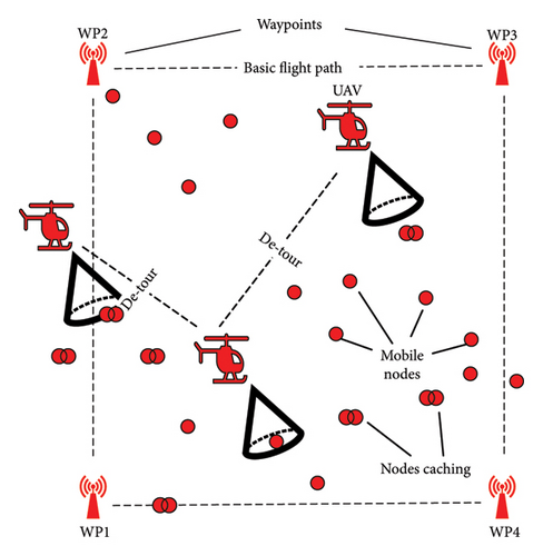
A discrete time event simulator was programmed in Java to carry out the simulations and experimentation in Reference [21] which was later enhanced in this study. We use the same approaches of direct and indirect caching. Figure 1 illustrates our enhancement to the previous work, allowing for detours.
- 1.
The UAV takes off on its mission and is expected to visit four static waypoints (with one being the take-off and landing point) that have also been enabled with caching to store information of mobile nodes if they come in contact with them.
- 2.
Upon hovering over these static waypoints, the UAV is expected to acquire all the information stored on these static caching points and continue on its path toward the next waypoint.
- 3.
If the UAV encounters one or more of the mobile nodes while flying on its initial path, it not only downloads that node’s data but in addition, if that node is carrying cached data of other nodes, it takes that on board as well. The node acquires this in the form of (meta − data).
- 4.
Each encountered node or set of nodes (based on meta-data) may now act as tentative waypoints according to their possible future location.
- 5.
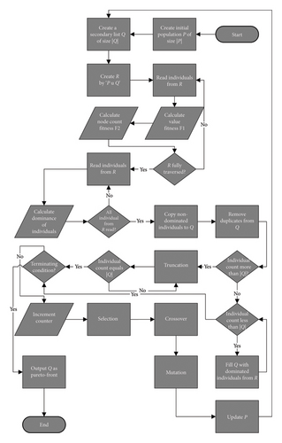
A list of waypoints (tentative and static) collectively forms an individual chromosome and each individual represents a path.
- 6.
An extra archive “Q”, i.e. expected to hold the nondominated solutions and ultimately the solutions that represent the Pareto Front, is also maintained alongside the main population archive “P”.
- 7.
A mega-archive “R” concatenated through the union of “P” and “Q” is also maintained and processed alongside “P” and “Q”. Each individual from “R” is evaluated against two objectives defined in the previous chapter, “Phase 2 Enhanced UAV Control System”.
- 8.
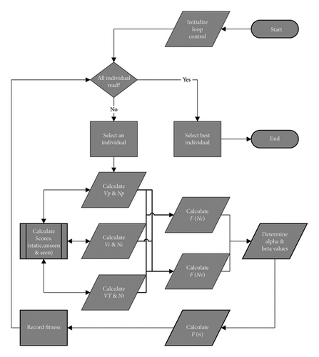
Fitness 1 from equation (5), representing the first objective “value of information” and Fitness 2 from equation (4), representing the second objective “count of nodes” on the path. For each individual chromosome, these are determined using a modified version of the fitness function given in equation (6) and Figure 3
- 9.
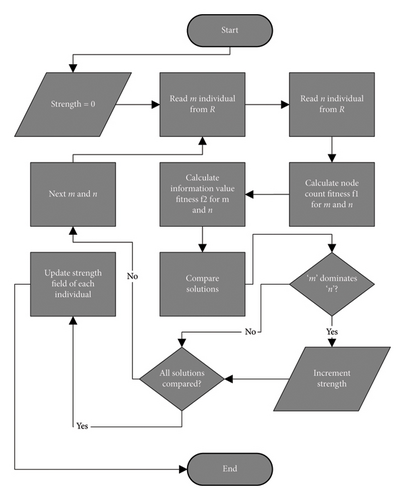
The strength, equation (7), representing the number of individuals dominated by an individual is then determined through the algorithm shown in Figure 4
- 10.
The dominance of each individual is calculated after determining the strength, raw fitness, density, and diversity of each individual, the details of which can be seen in Algorithm 2.
- 11.
The population on the Pareto front is managed using truncation and/or survival as shown in Algorithm 3.
- 12.
The terminating condition is then checked and if fulfilled, archive “Q” containing the nondominated solutions is presented as the Pareto front.
- 13.
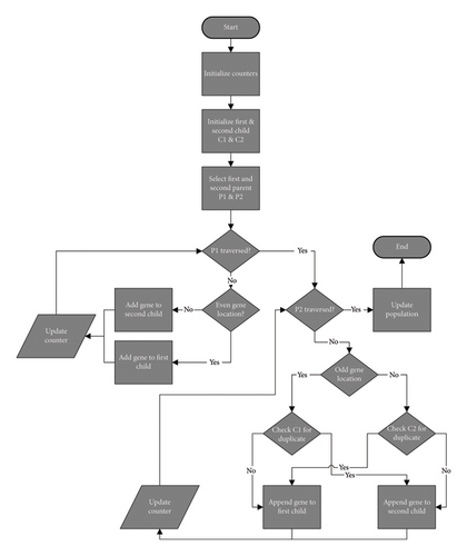
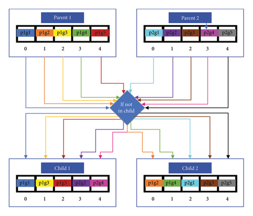
If the termination condition is not met, the algorithm continues and enters reproduction through selection, crossover, and mutation as shown in Figure 2.
-
Algorithm 1: SPEA-DUP (SPEA for DYNAMIC UAV PATHs).
-
Data:i = 0 ; P ; Q ; R ; non_dom_list.length;
-
Result:Pareto front
-
P⟵Popinit; /∗Initial population (Separate Algorithm) ∗/
-
QR⟵P ∪ Q
-
while:generation < maxdo
-
whileR.individual.next ≠ Nulldo
-
fitness1 = 1 − value_fitness(individual); /∗ equation (4) ∗/
-
fitness2 = 1 − nodecount_fitness(individual); /∗ equation (5)∗/
-
/∗ For GA, uses Algorithm in Figure 3∗/
-
end
-
Strength(R); /∗Algorithm in Figure 4: Strength ∗/
-
Dominance(R); /∗Algorithm 2: Dominance ∗/
-
count = non_dom_list.length
-
ifcount > |Q|; /∗Algorithm 3: Truncation & Survival ∗/
-
then
-
Truncation(R)
-
else
-
Survival(R)
-
end
-
Selection(Q);
-
CrossOver; /∗Algorithm in Figure 5: Crossover ∗/
-
Mutation; /∗Separate Algorithm for Swap Mutation∗/
-
Population − Update(P);
-
end
-
return Q;
-
Algorithm 2: Dominance.
-
Data:i = 0; k = 0; j = 1; R; Strength; Raw_Fitness = 0; distance = 0; diversity = 0; temp = 0
-
Result:_Fitness, Dominance
-
;
-
while:R.individual.next ≠ Nulldo
-
while:i < R.individual.dominators_list.lengthdo
-
temp = R.individual.dominators_list.get(i)
-
Raw_Fitness⟵Raw_Fitness + R.individual.getStrength(temp)
-
reset temp
-
i⟵i + 1
-
end
-
R.individual.RawFitness.set(Raw_Fitness); /∗R(i)∗/
-
while:j < R.lengthdo
-
x1 = R.individual.fitness1
-
y1 = R.individual.fitness2
-
x2 = R.individual.next.fitness1
-
y2 = R.individual.next.fitness2
-
distance = euclidean(x1, y1, x2, y2); /∗using the distance formula ∗/
-
R.individual.euclidean_list.add(individual.next.get( ), distance);
-
j⟵j + 1;
-
end
-
R.individual.euclidean_list.sort( ); R.individual.density.set(R.individual.euclidean_list.get(k)); /∗∗/
-
diversity = R.individual.density.get( ) + 2;
-
diversity = 1 ÷ diversity
-
R.individual.diversity.set(diversity); /∗D(i) ∗/
-
dom = R.individual.Raw_Fitness.get( ) + R.individual.diversity.get( )R.individual.Dominance.set(dom); /∗R(i) + D(i) ∗/
-
end
-
Algorithm 3: Truncation and survival.
-
Data:j = 0 ; i = 0 ; P ; Q ; R;
-
Result:Limited Pareto front
-
while:R.individual.next ≠ Nulldo
-
temp = R.individual.Dominance.get( )
-
iftemp < 1then
-
non_dom_list.add(R.individual); /∗list of nondominated solutions ∗/
-
else
-
dom_list.add(R.individual); /∗list of dominated solutions∗/
-
end
-
end
-
non_dom_list.sort( );
-
dom_list.sort( );
-
ifnon_dom_list.length > |Q|then
-
whilenon_dom_list.length > |Q|do
-
whilei < non_dom_list.lengthdo
-
whilej < non_dom_list.lengthdo
-
ifnon_dom_list(j).distance < non_dom_list(i).distancethen
-
minimum = non_dom_list(j); /∗find minimum σk∗/
-
i = jj = i + 1
-
else
-
minimum = non_dom_list(i); /∗find minimum σk∗/
-
end
-
end
-
end
-
non_dom_list.delete(minimum); /∗delete solution with min σk∗/
-
non_dom_list.length = non_dom_list.length − 1
-
end
-
Q.add( )⟵non_dom_list.get(i); /∗Update Q after truncation∗/
-
else
-
ifnon_dom_list.length < |Q|; /∗Survival∗/
-
then
-
while:i < non_dom_list.lengthdo
-
Q.add(i)⟵non_dom_list.get(i); /∗copy all non-dom solutions to Q∗/
-
i⟵i + 1
-
end
-
while:i < |Q|do
-
Q.append(i)⟵dom_list.get(j); /∗concatenate Q with dom solutions ∗/
-
i⟵i + 1j⟵j + 1
-
end
-
else
-
reset iwhile:i < non_dom_list.lengthdo
-
Q.add(i)⟵non_dom_list.get(i); /∗copy all non-dom solutions to Q∗/
-
end
-
end
-
end
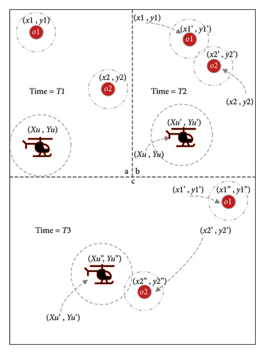
Since the sensor nodes are mobile, the UAV’s path must adapt in real time rather than relying on static node locations. To achieve this, the authors apply a predictive location model described in Algorithm 4 and illustrated in Figure 6. The UAV gathers meta-data (e.g., recent coordinates and timestamps) from nodes upon contact to predict future positions.
-
Algorithm 4: Estimating future position of moving nodes.
-
Data:int m1 = 0, m2 = 0, m = 0, c = 0, ynew = 0, xnew = 0;
-
Result:enew, Listcheckpoints
-
while:Nodecache.node.next ≠ NULLdo
-
Dronecache.append = Nodecache; /∗Transfer cache to UAV ∗/
-
end
-
while:Dronecache.node.next ≠ NULLdo
-
m1 = (Dronecache.node.current.y − Dronecache.node.last.y)
-
m2 = (Dronecache.node.current.x − Dronecache.node.last.x)
-
m = m1/m2; /∗Calculating the slope ∗/
-
c = Dronecache.node.current.x × m
-
c = Dronecache.node.current.y − c
-
ynew = (Dronecache.node.current.y + c)
-
xnew = (Dronecache.node.current.x + c)
-
ynew = Dronecache.node.current.y + (m1 × (Dronecache.node.current.T − Dronecache.node.last.T)) × Δ; /∗Predicting the x coordinate ∗/
-
xnew = Dronecache.node.current.x + (m2 × (Dronecache.node.current.T − Dronecache.node.last.T)) × Δ; /∗Predicting the y coordinate ∗/
-
genenew.x⟵xnew
-
genenew.y⟵ynew
-
Individual.append(genenew)
-
end
-
whileIndividualbest.gene.next ≠ NULLdo
-
gene1 = get.Individualbest.gene(i)
-
gene2 = get.Individualbest.gene(i + 1)
-
Listcheckpoints.append = bresenham(gene1, gene2); /∗using Bresenham’s algorithm ∗/
-
end
-
return Listcheckpoints; /∗return list of checkpoints between waypoints∗/
| State transitions | State 0 | State 1 | State 2 | State 3 |
|---|---|---|---|---|
| State 0 | 0/0 | 1/1 | 0/0 | 0/0 |
| State 1 | 0/0 | 0.975/0.95 | 0.025/0.05 | 0/0 |
| State 2 | 0/0 | 0.04/0.01 | 0/0 | 0.96/0.99 |
| State 3 | 0/0 | 0/0 | 1/1 | 0/0 |
3.1. Future Position Estimation and Trajectory Setup
The UAV uses these predictions to navigate closer to where a moving node will likely be. Since its communication range spans several hundred meters, it doesn’t need exact coordinates—just close proximity.
Figure 6 presents the process of future position prediction. In Figure6(a), objects O1 and O2 are shown at their initial coordinates, (x1, y1) and (x2, y2). In Figure 6(b), both objects move to new positions, (x1, y1) and (x2, y2), and encounter each other at time T2, where they exchange meta-data. Figure 6(c) illustrates their continued movement to (x1, y1) and (x2, y2), with O2 subsequently meeting the UAV. At T1, each object holds only its own data, including its current location and a null value for the last visited coordinate. By T2, the null entry is updated to reflect the previous position, while the current location is revised. Additionally, O1 and O2 exchange meta-data, enabling both to retain information about one another. At T3, this cycle continues, with O2 transferring its collected data and meta-data to the UAV upon contact.
Using the meta-data from Node O2, the UAV estimates (Algorithm 4 [31]) when and where it can intercept Node O1, based on the time difference between their last recorded contact. This estimate becomes a gene in the GA, treated as a potential waypoint. Bresenham’s algorithm [66] is used to compute the shortest route between these points.
3.2. Fitness Function
As shown in Figure 3, each individual in the population is analyzed for both and N⋆. The values are predefined or known at simulation start, while are derived from the individual’s genes. Alpha and Beta α, β control the weighting of these two objectives (see Table 3).
| Terms | Definitions |
|---|---|
| nT | Deployed nodes count |
| nC | Cached nodes at the UAV |
| VT | Total value of information |
| nC | Value collected by the UAV |
| nP | Node count on returned path |
| VP | Information value on returned path |
3.3. Strength
- 1.
Determine the initial fitness values Fitness 1 and Fitness 2 of each individual according to equations (4) and (5). These values, also termed as the initial solutions, are used to determine the significance of an individual over another.
- 2.
For each solution, we determine who it dominates and who it is dominated by. The number of solutions that a particular individual dominates becomes its strength value represented by STRINDIVIDUAL. A solution is said to dominate another provided that for each objective, the solution has a fitness value better than the other. For example, a solution “m” having better fitness values than “n” other solutions stores “n” as its STRM value.
- 3.
Raw fitness as shown in equation (8) is determined using the strength value in equation (7) along with density and diversity.
- 4.
Collectively, the cumulative value of raw fitness and diversity is taken as the dominance score of an individual.
(7)(8)
3.4. Dominance
The dominance of an individual is defined by a cumulative term that is a composition of strength, raw fitness, density, and diversity of an individual. Strength, as explained previously, corresponds to the number of individuals being dominated by a particular individual. We use the strength of individuals to calculate the raw-fitness value for each individual. The raw fitness of an individual is the sum of strength values of all the individuals that dominate it. For instance, if an individual m is being dominated by n individuals, the sum of strength of all n individuals becomes the raw fitness of the m. Hence, a higher value is a poorer result and the nondominated individuals will hold the lowest values.
Notice that the dominance does not only depend upon the strength value and the raw fitness value of an individual even though these two values do provide some sort of a niching mechanism. The algorithm makes use of density and diversity in addition to raw fitness and strength in order to handle individuals that may have the same fitness values. Density (σk) is an entity calculated based on the Euclidean distance of solutions from each other on a two-dimensional plain. The distance of each individual from every other individual is determined and is sorted ascendingly. An arbitrary distance is then selected from the sorted distance list that acts as the density value of that individual. This arbitration is controlled and is determined by a control variable “k” that is assigned value equivalent to the square root of the mega-archive. The diversity is then calculated using the density value in the denominator aiming to keep the value less than one. This process can be thoroughly seen in Algorithm 2. The diversity and raw fitness collectively represent the dominance of the individual.
3.5. Truncation and Survival
- 1.
The number of nondominated solutions in the mega-archive “R” are greater than the size of the secondary archive.
- 2.
The number of nondominated solutions in the mega-archive “R” are less than the size of the secondary archive.
- 3.
The number of nondominated solutions in the mega-archive “R” are equivalent to the size of the secondary archive.
The first situation is resolved using an approach termed as truncation and the second is resolved through an approach we label as Survival, both highlighted in Algorithm 3. For the third situation, no special technique is required since it requires a direct copy of nondominated solution from the mega-archive “R” to the secondary archive “Q”. The output of all three situations produces and updated population. This population, if the maximum generations have not been reached, becomes the updated children population which further goes through the reproduction phase. If the number of generations has reached the maximum iteration count, the nondominated solution in the secondary archive “Q” are presented as the solutions on the Pareto front. In the case of truncation, the number of nondominated solutions in the mega-archive “R” is greater than the size of the secondary archive that represents the Pareto front. In this situation, we are required to filter and delete some nondominated solutions to accommodate the remaining. SPEA-DUP chooses to delete the solutions with the minimum distance value hence presenting a diverse set of solutions on the Pareto front. Deleting without the distance parameter risks losing the edge solutions, a common issue in other algorithms. In the case of survival, the number of nondominated solutions in the mega-archive “R” is smaller than the total size of the secondary archive. In this situation, the algorithm initially copies all nondominated solutions to the secondary archive “Q” and fills the remaining gap by populating it with dominated solutions in order of their density value. For the third case, since the sizes match perfectly, no truncation or survival occurs, and the solutions get copied one by one to the secondary archive from the mega-archive.
These algorithms have been embedded in our bespoke event-driven simulator as an extension to our previous work in Reference [31] where in addition to GA-AP, we have also introduced SPEA-DUP and have assessed the two against five different simulation scenarios with two variations (Table 2) of the node movement model, Levy 1 and Levy 2 in Section 4.
4. Simulation and Results
Experiments are built on model [21], incorporating both GA-AP and SPEA-DUP for on-the-fly path decisions. Path feasibility is judged by how well they satisfy the dual-objective fitness function. The simulation mimics animal movement (like elephants [67, 68]) using the Lévy walk model, where nodes travel at over 2 m per second and may group in numbers between 8 and 100. Node range, field size, and density (Table 4) follow benchmarks from References [69–72].
| Attribute | Definition | Value |
|---|---|---|
| Simulations | Experiment count per scenario | 10 |
| Simulation duration | Each experiment run time | UAV’s roundtrip (≈45 min) |
| Communication protocol | Data communication UAV ↔ nodes | [31] |
| Static waypoint positions | Coordinates in the field | [31] |
| UAV altitude & speed | Height and velocity of flight | Constant |
| UAV coverage radius | Beam radius projected on ground | 250 m |
| UAV energy | Flight time of UAV | ≈45 min |
| α& β | Equation (3) | 0.5 & 0.5 |
| Cx | Crossover probability | 0.7 |
| Pm | Mutation probability | 0.01 |
| Node speed | Moving velocity of nodes | ≈2 m/s |
| Node coverage | Coverage radius in 2D space | 80 m |
| Transfer time | UAV ↔ nodes | Instantaneous |
| Value of information | Information carried by nodes | High (3)/medium (2)/low (1) |
| Node distribution area (Nda) | Size of 2D field | 100 km2 |
| Node density (per 100 km2) | Number of deployed nodes | 24 |
| Node distribution % (H-M-L) | % of nodes carrying high-, medium-, and low-value information | D1 : 12.5 − 25 − 62.5 |
| D2 : 25 − 25 − 50 |
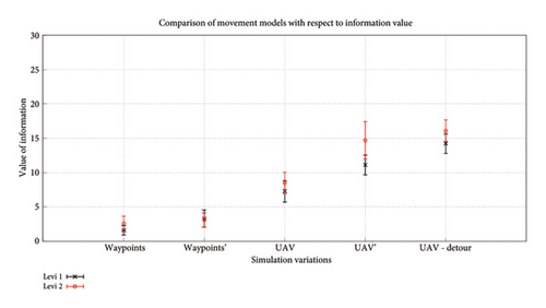
Five simulation variations are tested: Waypoints—UAV visits static waypoints to collect data from nearby mobile nodes. Waypoints’—Same as above, but with intra-node caching. UAV—UAV gathers data through direct contact with mobile nodes. UAV’—UAV collects data both directly and indirectly from nodes with caching. UAV—Detour—UAV dynamically changes path mid-mission using GA and predicted future node locations. All simulations assume unlimited node energy and storage, but UAVs are constrained by remaining flight time (residual energy). Any returned path that exceeds this limit is considered invalid. Each run starts with identical node positions, which then move freely.
Figure 8 shows how the fitness score varies based on different values of the control variables “alpha” and “beta” of the fitness function with respect to different node densities in the environment. A point to note here is that at higher node densities, we obtain a lower fitness value specially when we only consider the control variable “alpha” as represented by 1.0/0.0. This is because, although the node density is high and we have more high- and medium-value nodes compared to when we have a lower node density, the algorithm does not consider the value of information on the path and hence ends up returning paths that are strictly based on having more nodes. Since the distribution of the low-value nodes is greater than the medium- and high-value nodes, return of paths only having low-value nodes on them is a common occurrence. The fitness value starts increasing as we move from left to right, meaning we start including value of information as a parameter in the fitness calculation. Given that the returned path will now be based on the value of information on them, this will produce a fitness value higher than when only node count is considered.
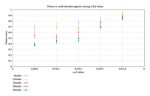
Figure 9 shows the effects of varying the values of the control parameter α & β on the convergence of the algorithm with a node density of 24. It can be seen that when the fitness function considers the value of nodes toward the determination of a fitter individual, the algorithm starts at a higher fitness value as a node of higher value is selected when the algorithm executes. This is when we set the alpha and beta parameters to 0.0/1.0. The converse of this can also be seen if we only consider the count of nodes for fitness. This is observable through the alpha and beta values of 1.0/0.0. Other combinations of alpha and beta have also been plotted. It can also be seen that even across different values of alpha and beta, the convergence of the algorithm happens well within 50 iterations of the algorithm. There is some slight delay in convergence when we start considering the value of the nodes in the fitness function mainly because though the number of nodes captured may not change or effect the convergence, the different values capture certainly will. While this might not always be the case, it occurs as the algorithm is able to locate nodes that carry higher value of information.
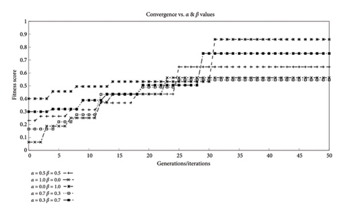
Figure 10 shows the convergence of the algorithm at different crossover and mutation rates. Both the crossover rate Cx and the mutation rate Pm lie within the intervals [0, 1]. The crossover rate determines the probability of a crossover to occur. A higher value means a higher likelihood of crossover to occur during the iterations of the algorithm. Hassanat et al. [73] suggest the typical crossover values lie within 0.5–1.0; hence, we have selected three values within that range. The same applies to the mutation rate. A higher value means more likelihood of mutation during the iterations. However, too high of a value is generally harmful as for optimal performance and can result in a random search hence [74] suggests based on his research that a value between 0.001 and 0.05 proves optimal and has been observed as being used across different researches based on GAs. Hence, we have selected three mutation rates within this range.
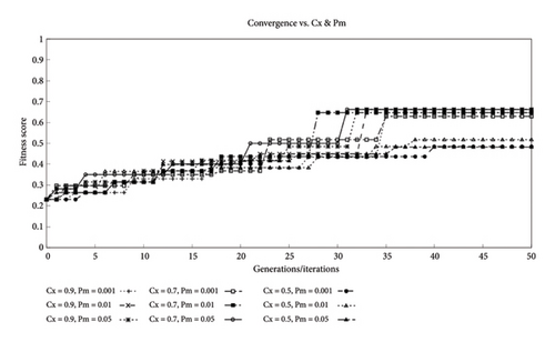
Figure 11 shows the effects on convergence of our algorithm with the variation of node density in the environment. As obvious from the results, even across different variations of node density, our algorithm is able to successfully converge within 50 iterations. Results also suggest that with higher node densities or distribution across the field, the algorithm takes more generations to converge. This however is not something that we are concerned with as the results suggest that the number of nodes where this will certainly be the case is significantly higher than our scenario. Our consideration is based on the fact that the type of animals in our study does not exist in a territory in large numbers. In addition, even with a higher node density, the setup does not guarantee knowledge of each and every node in the system and hence relies on the successful contact of the UAV with a node having metadata which is later utilized to calculate detours.
Figure 12 presents the plot of the solution archive “Q” with respect to the Pareto arc each solution belongs to. The nondominated individuals build up the Pareto front. Behind the Pareto front lie other Pareto arcs which can become fronts if the nondominated solutions are ignored. A solution is said to be nondominated if its F (NV) and F (NC) values collectively are the lowest among all other solutions, Algorithm 2. The dominance score shows that there exist only two solutions that are nondominated. The remaining archive is filled with the next dominated solutions. Hence, the main “Pareto front 1” only shows two solutions to which all others converge.
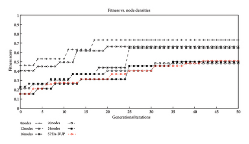
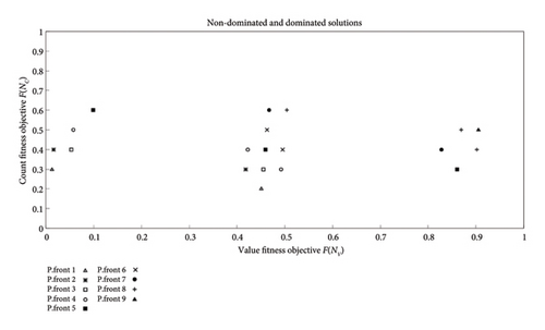
Figure 13 illustrates the UAV performance using SPEA-DUP under deployment D1, with alpha and beta both set to 0.5. The UAV—Detour strategy captures more nodes than UAV, but fewer than UAV’. This is because Detour relies on contact, while UAV’ benefits from indirect data transfer via caching. The results are quite similar for GA-AP and SPEA-DUP in almost all cases except UAV–Detour. With detouring, SPEA-DUP provides a slightly better percentage of captured nodes compared to a GA-AP showing that SPEA-DUP not only provides a better alternative to a GA but enhanced outcomes as well. Figure 14 shows a side-by-side comparison of GA-AP from [31] and SPEA-DUP in terms of percentage of nodes captured.
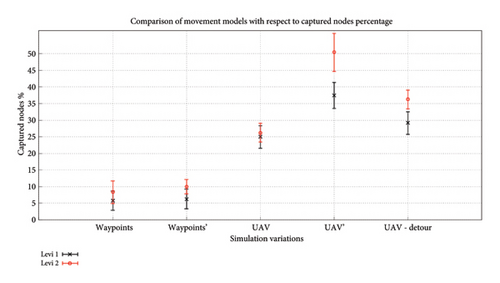
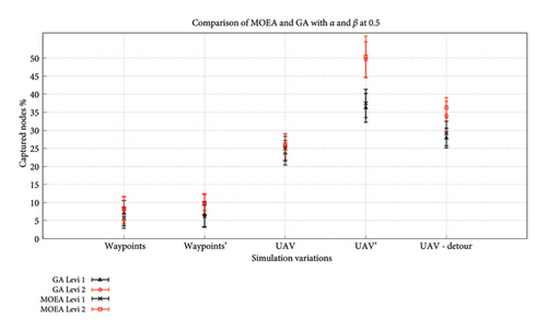
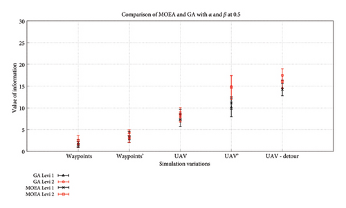
Figure 15 shows the returned value of information from the trip by the UAV for distribution D1. In both the cases of GA-AP from [31] and SPEA-DUP, Waypoint and Waypoint’ show little to no difference. This is because the attribute variation in the simulation for the two cases in terms of the movement model does not guarantee a contact with the static waypoints. UAV – Detour due to the consideration of the information value in the fitness function shows more valuable information collected. The long-step Levy model also assists in this as now the nodes cover more ground and hence their encounter probability increases as well. The side-by-side comparison of GA-AP and SPEA-DUP in Figure 16 shows that the difference effects caching and detouring for GA-AP but SPEA-DUP returns consistent results for both walks, with slightly better results for the searching phase. This again puts SPEA-DUP in the spotlight of the preferable algorithm choices out of the two as it presents a lot more information in single run which would otherwise require multiple executions of GA-AP.
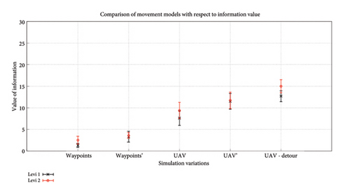
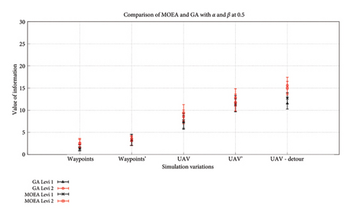
Figure 17 shows the returned value of information from the trip by the UAV for distribution D2. We see a slight improvement when comparing it to the statistics of D1. This is expected as the distribution now has a greater number of high- and medium-value nodes and hence their cumulative value at the end of the trip is expected to be higher than before as well. The side-by-side comparison of GA-AP and SPEA-DUP in Figure 18 again shows consistency in the results produced by both the algorithms. While in some variations, one might seem better than the other but overall, the results produced by both the algorithms fall within the confidence interval of each other suggesting that the results could be quite similar/same in different environments.
5. Conclusion
Overall, results confirm that evolutionary algorithms are highly effective for real-time path and trajectory planning, especially when targets are moving, and static planning isn’t viable. The importance of the data can change and hence new preferences and aims might need to be accomplished dynamically. The model allows mission objectives to adapt dynamically through the fitness function. We also show how different mobility patterns affect performance and highlight the value of caching. The effects of intranodal caching and its advantages with UAV data collection have been elaborated. While full data caching helps, lightweight metadata can be a resource-saving alternative. Both GA-AP and SPEA-DUP yield promising results, though GA-AP requires multiple runs for optimal tuning, whereas SPEA-DUP can return diverse solutions in a single execution. Lastly, our hybrid crossover model and future position prediction warrant further exploration with research work on performance evaluation against existing approaches.
Nomenclature
-
- UAV
-
- Unmanned aerial vehicle
-
- MOEA
-
- Multiobjective evolutionary algorithms
-
- MANETs
-
- Mobile ad hoc networks
-
- WSNs
-
- Wireless sensor networks
-
- GA
-
- Genetic algorithms
-
- GA-AP
-
- Genetic algorithm-aerial paths
-
- SPEA-DUP
-
- Strength Pareto evolutionary algorithm for dynamic UAV paths
Consent
All authors provide consent for the publication of identifiable details, including images, charts, algorithms, or relevant information within the text, in the aforementioned journal and article.
Conflicts of Interest
The authors declare no conflicts of interest.
Funding
This research did not receive any specific grant from public, commercial, or not-for-profit funding agencies.
Open Research
Data Availability Statement
Data supporting the findings of this study are available from the corresponding author, Umair B. Chaudhry, upon reasonable request.


